
Abstract
Millions of traffic accidents occur worldwide each year, resulting in tens of thousands of deaths. The primary cause is the distracted behavior of drivers during the driving process. If the distracted behaviors of drivers during driving can be detected and recognized in time, drivers can regulate their driving and the goal of reducing the number of traffic fatalities can be achieved. A deep learning model is proposed to detect driver distractions in this paper. The model can identify ten behaviors including one normal driving behavior and nine distracted driving behaviors. The proposed model consists of two modules. In the first module, the cross-domain complementary learning (CDCL) algorithm is used to detect driver body parts in the input images, which reduces the impact of environmental factors in vehicles on the convolutional neural network. Then the output images of the first module are sent to the second module. The Resnet50 and Vanilla networks are ensembled in the second module, and then the driver behavior can be classified. The ensemble architecture used in the second module can reduce the sensitivity of only a single network on the data, and then the detection accuracy can be improved. Through the experiments, it can be seen that the proposed model in this paper can achieve an average accuracy of 99.0%.
Introduction
According to a report published by the World Health Organization (WHO) [1] in 2020, approximately 1.35 million people lost their lives in the traffic accidents in the world every year. In most countries, road traffic collisions account for about 3% of the gross domestic product (GDP). Distractions from inside the vehicle contribute to 55.5% of accidents, and the errors of the driver are responsible for up to 90% of road accidents [2–4]. The National Highway Traffic Safety Administration (NHTSA) reports that almost one in five traffic crashes are caused by distracted drivers, and the most common distraction is the use of the mobile device. While traffic accidents are caused by various factors, driver errors are a significant contributor [5]. The losses caused by traffic accidents affect individuals, families, and the nation significantly, which can be partly avoided by detecting the distracted driver behaviors using some technologies.
Distracted driver can be classified into three types: cognitive, visual, and manual distractions [6]. Cognitive distractions are related to brain activity, such as being distracted or lost in thought, which cannot be identified by the driver’s external postural characteristics, even if the driver is in a safe driving position. Visual distraction occurs when a driver takes his eyes off the road and looks at the scenery outside or inside the vehicle. Manual distraction is closely related to distracted driver behaviors, such as the driver’s hand and body posture. According to the research, manual distractions are the main cause of traffic fatalities [6]. Therefore, detecting driver manual distractions is the main focus of this paper.
Currently, three main categories of techniques are used to identify and classify distracted driving behavior. Research can be conducted using one of these methods or a combination of methods. The first type of detection method uses the driver’s physiological signals, which requires the use of various sensors [7, 8] such as EEG (electroencephalogram), ECG (electrocardiogram), EOG (electrooculogram), and heart rate signals. This method extracts features from the physiological signals to determine whether the driver’s behaviors are distracted or not. However, this method requires the driver to wear relevant monitoring devices, which can affect the safety of the driver. Moreover, it is challenging to provide quantitative and objective criteria for judging the driver’s behaviors according to the physiological signals due to individual difference and environmental conditions [9].
The second type of detection method uses the vehicle data collected by sensors installed in the vehicle, such as acceleration, deceleration, steering angle, vehicle heading angle, speed, and steering data, etc. This method focuses on monitoring and extracting the signal characteristics of the vehicle control data to judge distracted driver behaviors. However, this detection method requires the use of expensive hardware devices to obtain the driving data of the vehicle itself, and it is only effective under certain specific conditions [10].
The third type of detection method is the machine vision method. The facial expressions, eyes, and body movements of the driver can be captured by installing cameras in the vehicle. The pre-trained Convolutional Neural Networks (CNN) are used to extract driving features from the images to identify distracted driver behaviors in the references [11–13]. Machine learning algorithms account for 60% of the driver behavior classification methods [14]. The deep learning method is used in this paper to classify distracted driver behaviors.
The CNN shows significant advantages in image processing. There are many successful CNNs, such as VGG, AlexNet, GoogleNet, and ResNet etc. In this paper, an ensemble deep learning-based model for distracted driver behavior detection is proposed. The model consists of two modules: the detection module of driver body parts and the classification module of driver behavior. The detection module of driver body parts uses the CDCL algorithm [15] to detect the driver’s body, which can reduce the influence of environmental factors on the recognition accuracy. The images output by the first module are provided to the classification module, which incorporates the Resnet50 network and the Vanilla network. The output of these two networks is provided to the ensemble algorithm to obtain the final behavior classification, which reduces the sensitivity of individual networks to the input data.
The rest of this paper is summarized as follows: Section 2 introduces the related work in this paper, Section 3 presents the theoretical basis, Section 4 presents the proposed model, Section 5 gives the experiments and the results, and Section 6 concludes the paper and discusses the future directions.
Related work
Wanghua Deng et al. [16] proposed a system for assessing driver fatigue levels, which consists of three parts. Firstly, the system recognized and tracked the driver’s face using the Multiple Convolutional Neural Networks (CNN)-kernelized correlation filters (KCF) (MC-KCF) algorithm, which combined CNN and KCF algorithms. This algorithm reduced the impact of complex environments on the system. Secondly, the Dlib algorithm is used to identify 68 key points on the face to localize the mouth and eye regions. Finally, the system evaluated the driver’s sleepiness based on the eye and mouth states, using three different standards: blink frequency, eye closure duration, and yawning. The system achieved an accuracy of approximately 92% on the dataset collected by the authors. However, a drawback is that each frame of the video data needs to be pre-processed to meet the face-tracking requirements.
Mohammad Shahverdy et al. [17] proposed a method based on convolutional neural networks (CNN) to detect distracted driver behaviors from vehicle motion patterns. The system utilized an On-Board Diagnostic (OBDII) adapter to collect vehicle drive data from the Engine Control Unit (ECU), which was then converted into images using the Recurrence Plot (RP) technique. These images were then input into the CNN to identify the distracted driver behaviors. The authors achieved a high classification accuracy of 99.95% on their collected dataset. However, the method can also be further optimized by adjusting the size of the time window.
Hesham M. Eraqi et al. [6] proposed a driver distraction recognition model based on the convolutional neural network. The model utilized the skin segmentation algorithm to preprocess driver images and extract the driver’s face and hands. Four convolutional neural networks were employed for training. The outputs of these models were provided to an ensemble learning algorithm to obtain a final output by putting them through a SoftMax classifier, which achieved a classification accuracy rate of 84.64% on the AUC dataset. However, the drawback of the model is that it requires manual marking of the driver’s hands and face for detection.
Furkan Omerustaoglu et al. [18] proposed a two-stage method that utilized both driver image information and driving vehicle data to enhance the accuracy of detecting driver distractions. In the first stage, the CNN model is trained by transfer learning and fine-tuning methods. The image information was input to determine the optimal performing CNN model. Meanwhile, the driving vehicle sensor data is processed using a long short-term memory (LSTM) network to distinguish normal driving from distracted driver behaviors. In the second stage, the CNN model that processes image information was combined with the predicted LSTM model that processes driving vehicle sensor data to form the final LSTM model. The LSTM model determined the final driver behavior. The method achieved an accuracy rate of 85% on the dataset collected by the authors, but it has a high of hardware consumption.
Chaoyun Zhang et al. [19] proposed the interwoven deep convolutional neural networks with multi-stream architecture to classify driver behavior. The architecture used driver images taken from different views and the optical flows based on the images as inputs to the convolutional neural network, extracted features from multiple angles, and performed feature fusion. This built a tight ensembling system, which significantly improved the robustness of the model. A temporal voting scheme was also introduced to reduce the probability of misclassification. This model achieved an accuracy rate of 73.97% for nine different driving behaviors of drivers and an accuracy rate of 81.66% for five aggregated behaviors on the dataset collected by the authors. The only shortcoming is that the experiment was conducted on a dataset collected in a simulated car environment.
Ardhendu Behera et al. [20] developed a multi-stream LSTM (M-LSTM) network for recognizing driver behaviors. The M-LSTM network utilized both image information and temporal information of the image. The model employed pre-trained models and ensemble learning methods. The model extracted features at different levels of the input information to recognize driver behaviors, including driver body parts and driving environment. The model achieved an accuracy of 52.22% on the AUC distracted driving dataset and 91.25% accuracy on State Farm distracted driving datasets. However, the model can further optimize the M-LSTM network to improve detection accuracy.
A Ezzouhri et al. [21] proposed a deep learning model with greater robustness to detect driver behaviors, and the model was divided into three modules. The first module was the segmentation module. The original images were input to the segmentation module to identify the key parts of the body. The second module was the mapping and image generation module, which removed the irrelevant information from the original image and generated the new image. The third module used the VGG-19 network to detect distracted driver behaviors. The generating images of the second module were input to the VGG-19 network. The generalization ability and robustness of the model were verified on several datasets. The model achieved 96.25% accuracy on the dataset constructed by the authors. In the future, the driver’s images of different ages and races can also be added to the dataset used for the experiments.
CHEN HUANG et al. [22] proposed a hybrid CNN framework (HCF). The framework contains three modules. The first module used pre-trained models to extract features, such as ResNet50, Inception V3, and Xception The second module was the feature connectivity module. This module connected the extracted features by the three pre-trained models to obtain comprehensive information. The third module was the classification module. The behavior was classified by using the Softmax layer. The class activation mapping technique was used to highlight feature regions of distracted behaviors during the experiments. The method achieved an average accuracy rate of 96.74% on the State Farm distracted driver dataset, but the computation time is long and the number of parameters is high.
Lei Zhao et al. [23] proposed an adaptive spatial attention mechanism-based system to detect distracted driver behaviors. The proposed system combines three convolutional neural network models based on the attention mechanism. The original images were input to the first network to extract features. The system used the class activation mapping technique to highlight the discriminative regions of behavior in the input image and then cropped the image to obtain region images. The distinguished regions of images were input to the next attention-based convolutional neural network. Finally, the system fused the output features of the three networks and then used a KNN classifier to classify distraction behavior. The system gradually highlights the distinguished regions of the original images. It improves the accuracy of the system classification. The system achieved 97% accuracy on State Farm distracted driver datasets. However, too many parameters significantly increase the runtime of the system.
Nesrine Kadri et al. [24] proposed a novel stacked LSTM recurrent neural network architecture for behavior classification. The Dempster-Shafer (DS) theory of belief function reduces the uncertainty of data and improves the accuracy of behavior recognition. The obtained f1-score reached 97%.
Tahir Abbas et al. [25] proposed ReSVM, a model that combines the deep features of ResNet-50 with Support Vector Machine (SVM) classifiers for driver distraction detection. This improvement can be attributed to some inherent advantages of support vector machines. Namely, it had good generalization capabilities, prevented overfitting, and can handle non-linear data efficiently. The improved model obtained an accuracy of 95.5% on the State Farm distracted driver dataset. However, this model does not take into account the effect of the driving environment on its performance.
Theoretical foundations
Body segmentation algorithm
Since the CNN classification model discriminates all pixels of the input image, the driver images contain the driver’s body parts (including the head, body parts, arms, and hands) and the driving background (including the cabin, seat, vehicle’s various components, and external environment). The driving backgrounds are varied and cluttered, which cannot provide useful information about driver distraction to the CNN model. The images processed by the body part detection algorithm were input to the CNN model so that the model’s attention was focused on relevant regions, such as the driver’s body parts. It helps to provide driver distraction pixels of information and improve detection accuracy.
Body part segmentation is a challenging problem in the field of image segmentation. In this paper, the CDCL algorithm is used to segment the body parts of drivers. Detection of body parts aims to detect a person in an image as multiple semantically consistent regions (head, arms, legs) and highlights interested regions.
CNN
For a given image, two pixels that are close to each other are similar. In a convolutional neural network, each pixel is connected to a neuron. It rapidly increases the computational load. CNNs make image processing controllable at the computational level by filtering the connections between neurons based on similarity. For a given convolutional layer, instead of connecting each input to each neuron, the CNN restricts the connections so that any neurons can only receive the input (3*3 or 5*5) of a small fraction from the previous layer. Thus, each neuron is responsible for processing one region of the image. This approach significantly reduces the computational effort of the network. Therefore, CNNs are selected for application in the regions of image recognition in this study.
VGG-16 is proposed by K. Simonyan and A. Zisserman of Oxford University in the paper “Very deep convolutional networks for large-scale image recognition” [26]. In the 2014 ImageNet Large Scale Visual Recognition Chall(ILSVRC) [27] competition, the model achieved 92.7% accuracy in the first 5 tests. The dataset contains more than 14 million images belonging to 1000 classes. It is one of the notable models submitted for ILSVRC-2014.
Vanilla network is the a simplest RNN, with a simple model structure, a small number of parameters, a single input, and a single output.
The Resnet network has more layers than the VGG network. Resnet is proposed by Kaiming in the paper “Deep Residual Learning for Image Recognition”. The model won first place in the ILSVRC-2015 classification task in 2015 and won first place in the ImageNet detection, ImageNet localization, COCO detection, and COCO segmentation tasks. The main contribution of the residual neural network is the discovery of the “Degradation” phenomenon and the invention of the “Shortcut connection” for the degradation phenomenon, which greatly eliminates the difficulty of training neural networks with too much depth.
Activation function
The activation function introduces a nonlinear element to the neurons, which allows the neural network to approximate any nonlinear function at will, allowing the neural network to be applied to a multitude of nonlinear models.
In deep learning, the commonly use saturated activation functions are sigmoid, tanh, ReLU, and softplus. sigmoid and tanh activation functions, whose derivatives tend to 0 when the value tends to infinity, and both have the problem of gradient disappearance. But the ReLU (Rectified Linear Units) is a non-saturated activation, which has great strength in preventing gradient disappearance. The Softplus function can be regarded as a smoothing of the ReLU function.
The purpose of this experiment is to identify distracted driver behaviors into ten categories, which is a multi-classification problem. The Softmax function is used in this study, which can “compress” a K-dimensional vector with any genuine number into another K-dimensional real vector. The output of the neuron is the ratio of the input of each neuron to the sum of the input of all neurons in the current layer. The output of each neuron is in the range of (0,1), and the sum of all outputs is 1. The larger the output probability of the neuron, the higher the probability that the neuron’s corresponding category is the genuine category. The equation of Softmax function in the text as Equation (1).
In multi-classification problems, the Softmax activation function is used in collocation with the categorical_cros cross-entropy loss function in general. The loss function evaluates the difference between the probability distribution obtained from the current training and the genuine distribution. It describes the distance between the actual output (probability) and the expected output (probability), i.e., the smaller the value of cross-entropy, the closer the two probability distributions are.
The label of each category is a 10-dimensional vector. The vector is set to 1 at the index position corresponding to the present value, and the rest is set to 0. The equation of Loss function in the text as Equation (2).
According to the formula find that since there are only two values of 0 and 1 to take. And when y i = 0, Loss = 0, when y i = 1, the Loss will presence a value. That means categorical_crossentropy focuses on only one result.
When training a neural network model, if the model has too many parameters and the number of training samples is too small, the trained model is likely to be overfitted. The overfitting problem is often encountered when training neural networks. The dropout [28] technique is proposed to resolve the overfitting problem. The key to the Dropout technique is to ignore the randomly selected neurons in some specific periods during the training process, which can alleviate the occurrence of overfitting more effectively and achieve the effect of regularization to some extent. Dropout technology lead to the network learning more robust features that help improve generalization errors.
Method
The architecture of the CDCL-VRE model proposed in this paper is shown in Fig. 1. The model consists of two stages. The first part uses the CDCL algorithm to detect the driver’s body parts. The second part uses the ensemble algorithm. The Resnet50 network and the Vanilla network are provided to the ensemble algorithm and ultimately determine the driver behavior.
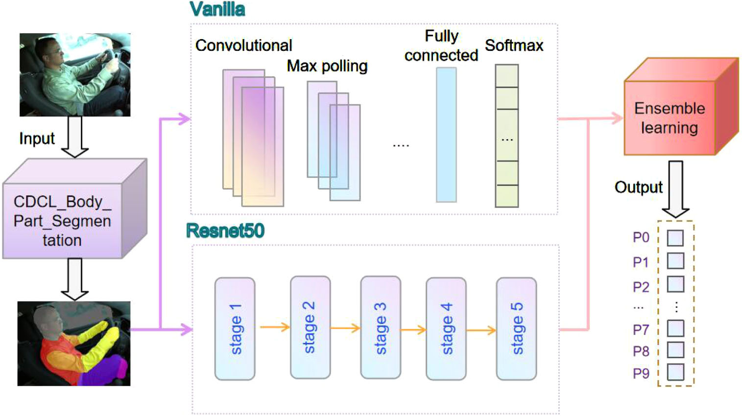
CDCL-VRE model architecture diagram.
Real and synthetic humans both have a skeleton (pose) representation, the skeletons can effectively bridge the synthetic and real domains during the training. The CDCL [15] algorithm takes advantage of the rich and realistic variations of the real data and the easily obtained labels of the synthetic data. The algorithmic framework is trained using a ResNet-101 network and contains two main components. The first component is the synthetic input trained to learn body parts and human poses in the synthetic domain. The second component for real input training shares the network parameters of the backbone, keypoint mapping head, and part affinity field head with the first component. CDCL algorithm solves the problem of data labeling at the pixel-level with the low cost.
The CDCL algorithm is used to detect each part of the human body (torso, arms, legs, head, etc.) more accurately despite the absence of any human markers or the poor quality of the pictures (low brightness, complex environment, the high number of people, etc.). The CDCL algorithm outperforms several other state-of-the-art methods that require human markers, including the method proposed in [29–35].
The input images are processed with the CDCL algorithm (the source code can be got in GitHub [36]). The comparisons of the images before and after detection are shown in Fig. 2.
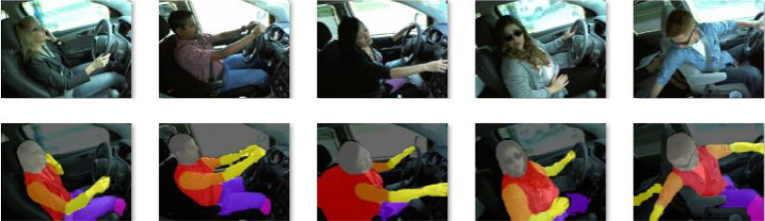
CDCL body part detection (the original images are listed in the first row and the images processed by the CDCL algorithm are listed in the second row).
VGG-16 pre-trained CNN architecture containing 13 convolutional layers (convolutional kernel size of 3×3) and 5 pooling layers (pooling kernel size of 2×2) to extract features. The last 3 fully connected layers are responsible for the classification task. Since the convolution kernel focuses on expanding the number of channels and the pooling kernel focuses on reducing the width and height, it makes the model architecturally deeper and broader while the computational effort increases slowly. The purpose of this model is to classify distracted driver behaviors into ten categories, so a fully-connected layer is added at the end of the classifier and the Softmax function classifies the final categories into ten classes and outputs the probabilities of the classes to which they belong.
The VGG19 network is based on the VGG16 network with three additional 3*3 convolutional layers. The pre-trained model is used and retrains only the fully connected layers, so the parameters to be retrained are the same for the VGG16 and VGG19 networks.
Vanilla network
The Vanilla network has a simple structure and a small number of parameters, consisting of 6 convolutional layers, 3 pooling layers, and 3 fully connected layers. Although the model of Vanilla Network is simple. However, it has low time complexity and high accuracy for driving image classification. The convolutional layer uses the convolutional kernel of 3*3 size and the ReLU activation function, and the pooling layer uses the pooling kernel of 2*2 size. Convolutional and pooling layers are responsible for extracting features. The fully connected layers are responsible for the classification task. Finally, the probability of belonging to each category is output by a Softmax function. The Vanilla network is summarized in Fig. 3.
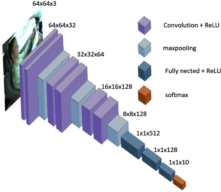
Vanilla network model architecture.
The depth of the network has a role in the feature representation and generalization ability, but simply stacking convolutional layers does not improve the generalization ability of the model well. resnet50 has significantly fewer training parameters compared to the VGG network, even less than the AlexNet network, despite the deepening of the number of layers. This is mainly due to removing the fully connected layers and instead using global average pooling.
Resnet50 network contains five stages. In the first stage, the input images successively go through the convolution layer, batch normalization, activation function, maximum pooling layer, and output; stages 2-5 alternately use two residual learning blocks, and two primary residual learning blocks are shown in Fig. 4. It is able to solve the problem of gradient disappearance during the training process.
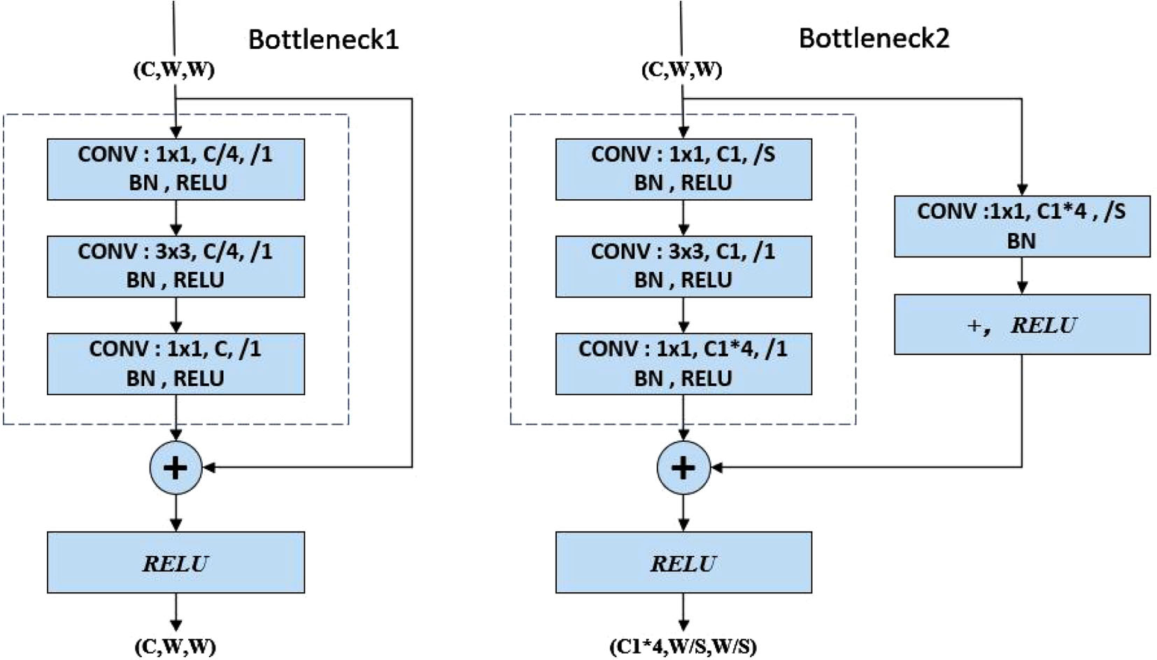
Two types of Bottleneck structures.
The input shape of Bottleneck1 is (C, W, W), which refers to the number of channels, width, and height of the input. Here the width and height are equal, so there are two variable parameters C and W. Assuming that the input shape (C, W, W) is x, F(x) can be got by the three convolution blocks, which is added with x to get (F(x) + x), and then a RELU activation function is used to get the output, which is still in the shape (C, W, W).
Bottleneck2 has four variable parameters C, W, C1, and S. The right side of Bottleneck2 has one more convolutional layer than Bottleneck1, assuming that the G(x) can be got by the right branch, the F(x) can be got by the left branch, and the two branches add up to get (F(x) + G(x)), and then go through a RELU activation function to get the output. The parameter S indicates whether the two 1×1 convolutional layers on the left and right of Bottleneck2 are downsampled; the parameters C and C1 indicate whether the first 1×1 convolutional layer on the left side of Bottleneck2 reduces the number of channels.
Pre-trained CNN architectures are trained by large datasets (the ImagetNet dataset [35]), and the pre-trained CNN architectures already can extract shallow base features and deep abstract features. The models can be initializers or extractors features for similar tasks. Since general experiments may not have big training datasets, the network is generally not trained from scratch. Using a pre-trained CNN architecture without fine-tuning, the network may run the risk of non-convergence, under-optimized parameters, low accuracy, weak model generalization ability, and over-fitting.
Ensemble learning
Distracted driver behaviors may lead to critical consequences and bring heavy loss to people’s families and society, so it is especially important to improve the accuracy of recognition for distracted behavior. With the increasing number of vehicles worldwide, it is possible to save countless lives and families as long as the accuracy rate is improved.
CNNs are highly capable of learning and very sensitive to the details of the training data. Different networks learn different features and different focus on the training datasets, and the output of prediction results will have a certain tendency. A better and more successful method is proposed to solve this problem, which trains multiple models instead of a single model, and obtains the final prediction by combining the results of each training model, called the ensemble method [38]. There are several ensemble methods available, such as weighted voting, simple averaging, and GASEN [39].
The weighted average ensemble algorithm is used in this paper. The contribution of each ensemble member is weighted by a factor indicating the trust or expected performance of the model. The weight value is a value between 0 and 1, so the sum of the weights of all ensemble members is 1.
Experiments and results
Dataset
In this section, the performance of the proposed model was validated by experiments, the module detected ten types of driving behaviors by multi-category classification. Ten behaviors include normal driving, typing with the right hand, answering the phone with the right hand, typing with the left hand, Answering the phone with the left hand, operating the radio, drinking, reaching behind, fixing hair or makeup, and chatting with passengers.
In the experiments, two publicly available datasets are used to evaluate the recognition performance of the models. The first dataset is the State Farm distracted driver dataset [40] to train the model and obtain classification accuracy. The second dataset is the American University in Cairo (AUC) distracted driver dataset [41] to validate the generalization ability of the model.
StateFarm’s dataset
The State Farm dataset is the first publicly available dataset for pose classification on Kaggle for detecting driver distracted contests. The dataset classifies driver postures into ten categories. The distribution of the State Farm dataset is summarized in Table 1. The image were input to the body part detection algorithm at a resolution of 320×240 RGB and were input to the neural network at a resolution of 64×64 RGB.
Distribution of distracted driver datasets
Distribution of distracted driver datasets
The dataset was divided into two non-overlapping datasets, with 80% of the entire dataset as the training set and 20% as the test set.
This study was inspired by the State Farm distracted driver detection. However, this dataset was only used for competition purposes, this dataset was used to train our model while another publicly available dataset was used to validate the effectiveness of the model proposed in this paper. The AUC distracted driver dataset. Collected in the real driving environment. the AUC dataset has 44 individuals, 29 males, and 15 females, from 7 countries: USA, Egypt, Germany, Uganda, Canada, Morocco, and Palestine. The videos were taken at different times of the day, in different cars, under different driving conditions, and with different drivers wearing different clothes [42]. The following Table 3 shows the distribution of images in the AUC dataset.
The comparison experiment of the activation function
The pre-trained CNN architecture and fine-tune method were used in this study. The parameters of the fully connected layers were retrained. The Adam optimizer was used in this study. The learning rate was set to 1 * e-3 when training the network pre-trained model; since the Vanilla network has few layers, a simple structure, and a small number of parameters. The Vanilla network was trained from scratch and the learning rate was set to 0.001.
Four activation functions were put into the model for training, and their accuracies are summarized in Table 2.
Comparison of the effects of activation functions
Comparison of the effects of activation functions
Table 2 shows that the ReLU activation function performs the best among the other activation functions. Because the ReLU function is non-saturated, which means there is no issue with gradient saturation. Although the ReLU function is not centered at 0, it has a gradient value of 0 in the negative direction, and weights are not updated during back-propagation. However, in the positive direction, the gradient value is 1. Additionally, the ReLU function is linear and can effectively solve the problem of gradient disappearance, leading to improved operational speed. As a result, The ReLU activation function was used for our model. The equation of ReLU activation function in the text as Equation (3).
Four pre-trained models were evaluated on the State Farm distracted driver dataset, compared to before and after using the body segmentation algorithm, and the accuracy and number of parameters for the four pre-trained models. The training results are summarized in Fig. 5.

Pre-trained network comparison chart.
As can be seen in Fig. 5, the classification accuracy of the four pre-trained models using the body segmentation algorithm is significantly improved compared to without the body segmentation algorithm, which proves the effectiveness of the body segmentation algorithm; at the same time, the number of parameters of the Resnet50 and Vanilla networks is significantly reduced compared to that of the VGG network and the accuracy is high, so the Resnet50 and Vanilla networks are selected to ensemble in this paper to reduce the sensitivity of individual networks to the data.
The State Farm distracted driver dataset was put into our model for experiments. The images of body parts were obtained by the CDCL algorithm and then input to the Vanilla network and Resnet50 network for training and testing, respectively. The variation of the accuracy and loss of the network with an increasing number of epochs is shown in Fig. 6.
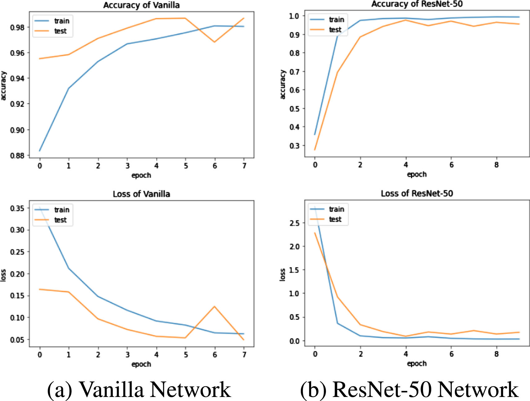
The variation of the accuracy and loss of the network with an increasing number of epochs.
The loss function decreases and the accuracy rate increases with the increase of training epochs from Fig. 8. The Vanilla model reaches the accuracy rate of 99.28%. The Resnet50 model reaches the accuracy rate of 99.46%.
The Vanilla network and ResNet-50 were ensembled in this paper for several training sessions, and the results of five randomly selected experiments are summarized in Table 3. The average accuracy is about 99.58%.
The results on the State Farm dataset
It can be observed from Table 3 that using the vanilla network for driver abnormal behavior classification alone, an average accuracy of 99.27% can be obtained on the State Farm driver behavior dataset. Using the ResNet-50 model for driver diastracted behavior classification alone, an average accuracy of 99.26% on the State Farm driver distracted dataset can be obtained. It is difficult to improve the accuracy any further by training two networks individually, and the ensemble of the two models achieves an average accuracy of 99.58%. The proposed model can reduce the sensitivity of a single network to the input data, and improve the detection accuracy.
The confusion matrix helps us to visualize the number of correct and incorrect predictions. It gives us an idea of how well the classifier model works on the test set. The confusion matrix forms the basis of most classification metrics, such as accuracy, precision, and recall, as these metrics are derived from the confusion matrix [43]. Figure 7 shows the confusion matrix of the two network models for ten classes of behavior recognition.
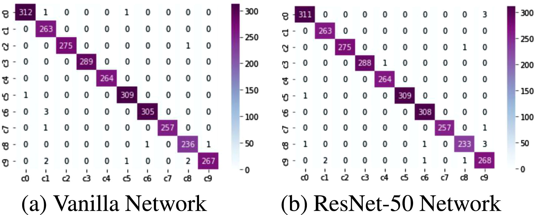
Confusion matrix.
In the confusion matrix output by the Vanilla network, The network misclassifies chatting with passengers as safe driving three times because drivers may keep their hands on the steering wheel and only turn their heads while chatting with passengers, which is very similar to the state of safe driving and prone to cause misclassification of the system; The Vanilla network misjudges the behavior of typing with the right hand as chatting with passengers behavior two times; The Vanilla network misjudges the behavior of chatting with passengers as fixing hair or makeup three times, which is because when chatting with passengers, drivers may have more behaviors about hand, sometimes with both hands on the steering wheel, which is also the reason why the network misjudges the driver’s behavior of chatting with passengers as normal driving behavior. The content of the driver’s chat with passengers and the driver’s state of driving the vehicle may cause the driver to behave in various ways. In the confusion matrix output by the Resnet50 network. Resnet50 network misjudges the behavior of chatting with passengers as safe driving two times, typing with the right hand as chatting with passengers behavior two times, and the behavior of fixing hair or makeup as chatting with passengers two times, which is similar to the reasons for misclassification by the Vanilla network.
The confusion matrix after using the ensemble algorithm is shown in Fig. 8.
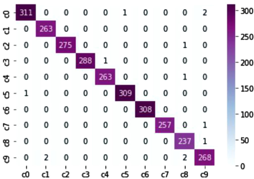
Confusion matrix of using ensemble algorithm.
By comparing the confusion matrices in Figs. 7 and 8, it can be seen that the ensemble learning algorithm reduces the misclassification rate. The Vanilla network misclassified chatting with passengers as normal driving behavior twice, which was reduced to once using the ensemble algorithm; The Vanilla network misclassified chatting with passengers as fixing hair or makeup behavior three times, which was reduced to once using the ensemble algorithm; The ResNet50 network misclassified typing with the right-hand as drinking behavior three times, which was reduced to zero using the ensemble algorithm; The ResNet50 network misclassified typing with the right-hand as normal driving behavior once, which was reduced to zero using the ensemble algorithm; The ResNet50 network misclassified adjust the radio as chatting with passengers behavior once, which was reduced to zero using the ensemble algorithm. The effectiveness of the ensemble algorithm was demonstrated, which reduced the sensitivity of individual networks to data and improved classification accuracy.
The evaluation metrics such as Precision, Recall, and F1-score can be calculated from the data in the confusion matrix with the equations in the text as Equations (4–6).
The Precision, Recall, F1-score, Support, micro avg, macro avg, weighted avg, and sample avg of the Vanilla network in each category of the test set are summarized in Table 4. The values of each category are above 0.98. The Precision, Recall, F1-score, Support, micro avg, macro avg, weighted avg, and sample avg of the Resnet50 network in each category of the test set are shown in Table 5.
The results on the State Farm dataset
The results on the State Farm dataset
The results of comparing the model proposed in this paper with other state-of-the-art methods using the same dataset are shown in Table 6. The method in this study outperformed other state-of-the-art methods in identifying driver distraction behavior.
Comparison with other methods
Comparison with other methods
The model proposed by Imen JEGHAM [15] used the SURF keypoint technique to detect driver body regions and used the K-NN method for classifying driver behaviors, obtaining an average accuracy of 70% on the State Farm dataset; The model proposed by Furkan Omerustaoglu [18] introduced a time series. They built a CNN model on the driver image data and an LSTM model on the time series of control data of the vehicle. Finally, the two models built were provided to the ensemble algorithm to obtain the final LSTM model and obtained 85.00% accuracy on the State Farm dataset; Ardhendu Behera [20] also introduced time series and used the driver image as well as the temporal information of the driver image to build an LSTM model on the State Farm dataset to obtain an accuracy of 91.25%; C. Huang [22] proposed the HCF framework using class activation mapping technique to highlight the region of interest of the pre-trained models, The features were extracted by three pre-trained CNN architectures: ResNet50, Inception V3 and Xception in parallel and were fused into a one-dimensional vector that was sent to the Softmax function for classification. An average of 96.74% was achieved on the State Farm distracted driver dataset. But the three pre-trained CNN architectures have a large number of parameters and high computational complexity; The ResneXt101-S2F model proposed by Lei Zhao [23] has a lower accuracy than the ResneXt101-S3F model, but is faster than the ResneXt101-S3F model, and it is difficult to balance the accuracy with the computational effort. The model proposed in this paper used a CDCL algorithm to highlight the region of interest of the CNN. The Resnet50 network and the Vanilla network were provided to the ensemble algorithm that determined the driver behaviors, and the model obtained an average accuracy of 99.58% on the State Farm dataset
The robustness and generalization of the model proposed in this paper were further evaluated using the AUC dataset. 80% of the dataset was used for training and the rest for testing for dividing the dataset. The authors of the AUC dataset used a temporal annotation mechanism to label the recorded videos. Each video frame was labeled as a category. However, by looking at the image markers, it can be noticed that in some cases the authors failed to correctly select the beginning and end of the video sequence, which led to some images being annotated with errors [21]. Therefore, we manually filtered all the classes. Removed and changed the incorrect video frames.
The manually processed dataset was applied to our proposed method. Five training results after several training sessions were randomly selected. The results are summarized in Table 7. The model achieved an average accuracy of 98.2%. Error annotations can interfere with the recognition of the model. The high accuracy of the AUC dataset in our model demonstrated the strong performance and generalization ability of our proposed model.
Training results on the censored AUC dataset
Training results on the censored AUC dataset
The proposed deep learning model reduced the influence of environmental factors on CNN. Earlier methods focused only on the driver’s face and body parts, ignoring the effect of environmental factors on the neural network. Therefore, the accuracy did not reach a high standard. The environmental factors were taken into account in convolutional neural networks in this paper. The CDCL algorithm was used to detect driver body parts, which allowed the neural network to focus the region of interest on the driver body parts. In addition, ensemble learning takes full advantage of the complementary qualities of the used models to provide more accurate outputs.
This experiment only detected driver body parts, which were not extracted directly. In the future, the body part segmentation algorithm needs to be further optimized to extract driver body parts directly and further reduce the influence of environmental factors on the neural network has the potential to achieve higher accuracy rates; The network used in this paper can be improved by adding an attention mechanism that makes the model focus attention on the driver’s body parts, but adding an attention mechanism to the network does not necessarily result in a performance improvement, because the model’s performance may be affected by the dataset, the model, and the location of the attention module; Although the models in this paper has very few parameters and good performance, there are still other models that have fewer parameters and can be applied in the driver behaviors detection, such as SqueezeNet, MobileNet, and ShuffleNet, etc. which can be studied and improved in the future.
Data availability statement
The datasets generated during and/or analysed during the current study are available from the correspoding author on reasonable request.