Sage Journals: Discover world-class research

Abstract

Accurately estimating concrete mechanical parameters using artificial intelligence-based methods can save time and energy. Existing nonlinear relationships between concrete components have entered uncertainty in the estimation of hardness properties of the slump and compressive strength as one of the most important parameters in concrete design. Employing regular approaches to use AI models individually in estimating dependent variables has been adopted in many studies. Therefore, the current study has aimed to develop predictive models in two categories of ensemble and hybrid frameworks to predict the hardness properties of high-performance concrete (HPC). In this regard, models based on Support Vector Regression, Decision Tree, and AdaBoost Machine learning were coupled with a metaheuristic optimization algorithm Chaos game optimizer (CGO). Linking three predictive models as well as tuning their internal settings via optimization algorithm could generate various types of hybrid and ensemble models. By assessing the results of the proposed models for compressive strength, the performance of ADA-CGO hybrid models was calculated higher than the ensemble model of SVR-ADA-DT, with 1.22% and 166% percent difference in terms of R² and RMSE, respectively. Also, for predicting Slump, other hybrid models appeared with weaker performance than the ensemble model, with an average difference of 40.66% in terms of the MAE index. Generally, using advanced types of individual models, including ensemble and hybrid, indicated boosted performance accompanied by low-cost modeling processes.

Keywords

High-performance concrete compressive strength and slump AdaBoost support vector regression decision tree Chaos game optimizer.

1 Introduction

Concrete is widely employed as a building material due to its being readily economical, available, and widely applicable. However, their fragility is the main weakness when used in seismic zones. Fairly low resistance and low tensile strength to propagation and cracking are the main drawbacks that must be crushed [1]. The present scenario creates a great need for concrete with key qualities like high strength, high workability, durability, and toughness [2]. A few sorts of concrete contain High-Performance Concrete (HPC), high-strength concrete (HSC), and Fiber Reinforced High-Performance Concrete Composite (FRHPCC). It has superior effects compared to conventional concrete [3].

High-Performance concrete (HPC) is described as concrete with compressive strength (CS) greater than 80 MPa and containing silica fume generally 5-15% by mass of total cementitious material, cement scope in the range of 450 –550 Kg/m³, or sometimes fly ash or crushed granular blast furnace slag. Always a superplasticizer and at very high doses reduces water range. The low water-cement ratio is due to the need for durable and compact mixtures. In recent years, considerable improvements in the concrete’s mechanical properties containing steel fibers have been documented [4].

Certain chemical and mineral additives like superplasticizers and fly ash are used in HPC mixtures to improve concrete durability, workability, and strength. HPC is mainly utilized in tunnels, bridges, hydroelectric power, and skyscrapers. The HPC mix design process needs several trial mixes to construct concrete that satisfies the demands of the environmental and structural construction project [5]. This often leads to a loss of material and time. In the design of HPC, compressive strength (CS) and Slump as hardness properties are the most essential parameters. They have a strong relationship with the general concrete’s quality. Accurate and early estimation can save money and time by developing the necessary data design [6, 7].

Traditional processes may not be appropriate for estimating the Slump and CS of HPC. Due to the relationship between concrete compressive strength and components being highly nonlinear makes it difficult to obtain a precise regression equation [8 –10]. Several predictive models for the CS and Slump of different sorts of concrete have been generated employing machine learning (ML) techniques containing support vector machine (SVM) [11, 12], artificial neural network (ANN) [13 –16], Adaptive Boosting (ADA) [17], and the ensemble method [18].

Bhatti et al. [19] demonstrated the applicability of artificial neural networks for estimating slumps in high-performance concrete. Yeh [20] showed the ability of an artificial neural network to represent the effect of each material feature on the Slump of concrete. Yu et al. [21] suggested a new method according to SVM to predict the HPC compressive strength. Behnood et al. [6] used the M5P model tree algorithm to model the HPC compressive strength. Mousavi et al. [22] generated a model based on gene expression programming (GEP) to predict the HPC compressive strength.

As the novelty of the present paper, different types of models, namely hybrid and ensemble, were considered to master the capability of AI-based frameworks in predicting the hardness properties of high-performance concrete samples. In fact, the current study has aimed to develop Freund and Schapire’s [23] AdaBoost algorithm as the first observed boosting algorithm and one of the most commonly utilized and studied methods in many prediction fields. Over the years, various tries have been created to “explain” AdaBoost as a learning algorithm to understand how, when, and why. A fundamental comprehension of the nature of learning can advance the field in general and concerning specific algorithms and phenomena. Certainly, this was a lesson in Vapnik’s life’s work.

Also, using the Decision tree (DT) technique is one of the strong approaches widely employed in different works, like image processing, identification of patterns, and machine learning [24]. DT is a successive model that unites a series of basic tests cohesively and efficiently, where a numeric feature is compared to a threshold value in each test [25]. The conceptual rules are much easier to construct than the numerical weights in the neural network of connections between nodes [26, 27]. It is noteworthy that DT is used mainly for grouping purposes. Furthermore, another model of the study, Support vector regression (SVR), attempts to underrate the bounded generality error to reach generalized execution. SVR uses a threshold value-ɛ lower than a loss function to discipline errors. These loss functions usually result in scanty representations of decision rules. It provides algorithmic and representative benefits. Support vector machines (SVMs) have been applied to diverse pattern-mention applications like image recognition and text classification and have been observed to extend to the analysis of regression [28 –30]. On the other hand, to improve the results of the models, Chaos game optimization (CGO) is presented in this paper as a new metaheuristic algorithm for adjusting restrained technical design and mathematical issues. CGO is also developed on the basis of some codes of chaos theory, and the fractal structure is outlined by the chaos game methodology, together with the problem of fractal self-similarity [31].

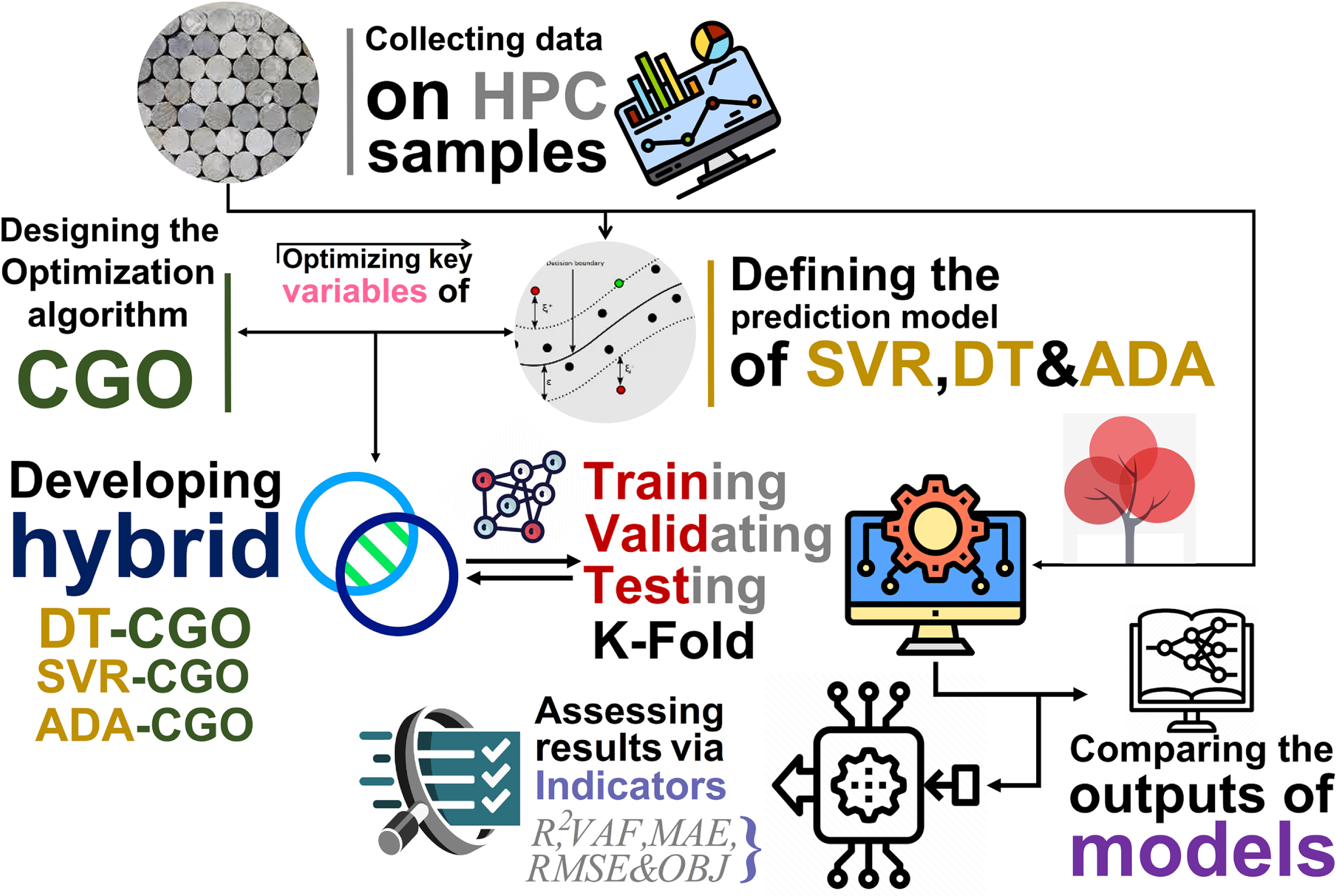
Various combinations of presented models and optimizers will define a holistic framework in generalizing hybrid and ensemble models. In this regard, the capability of each component is crispened clear to show the framework performance in anticipating the mechanical features of concrete samples. In light of better showing the potentials of developed hybrid and ensemble models, several evaluative indices were employed, and the results were compared relative to each other, plus the K-fold cross-validation stage. The overall view of the current paper’s stages to reach the end has been indicated in Fig. 1.

Fig. 1

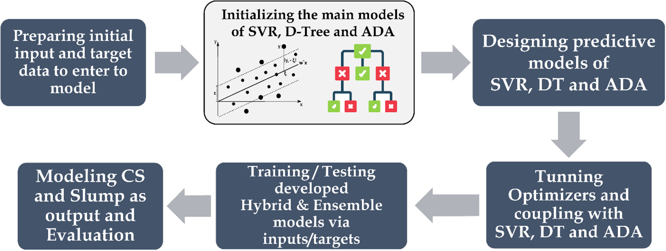
The schematic view of the current paper stages in the prediction of hardness properties.

2 Materials and methodology

2.1 Data gathering

An initial dataset is deemed the obligatory component to investigate the capability of developed models. In light of assessing both hybrid and ensemble frameworks, a dataset from the literature [32], conducted by Lim et al (2004), containing 189 high-performance concrete (HPC) compounds were used. The inputs as HPC constituents are binder (B), water (W), silica fume (SF), fine aggregate to total aggregates ratio, fly ash (FA), silica fume (SF), superplasticizer (SP), air entraining agent (AE), as well as outputs compressive strength (CS) and Slump that are considered as targets. It should be noted that the slump-measured hardness characterization of concrete samples was performed after 28 days. Experiments were conducted in South Korea to measure the quantity of materials except for silica fume. Selected Portland cement conforming to ASTM Type I standards. In addition, a special density 2.7, grain size 7.2 coarse aggregate was produced from crushed granite, mostly 19 mm. A fine silica sand aggregate with a specific gravity of 2.61 and a fineness coefficient 2.94 was also produced. Naphthalene superplasticizers have been used as water reducers to control concrete’s water-to-binder (W/B) ratio. Class F silica fume and fly ash are produced in Norway. Also, the slump test passed the ASTM C 143-90a standard immediately after mixing. The test was conducted according to the ASTM C 231-91b standard and measured the incoming air mixture. Figure 2 shows the input and target data regarding their frequencies and cumulative quantity percentage.

Fig. 2

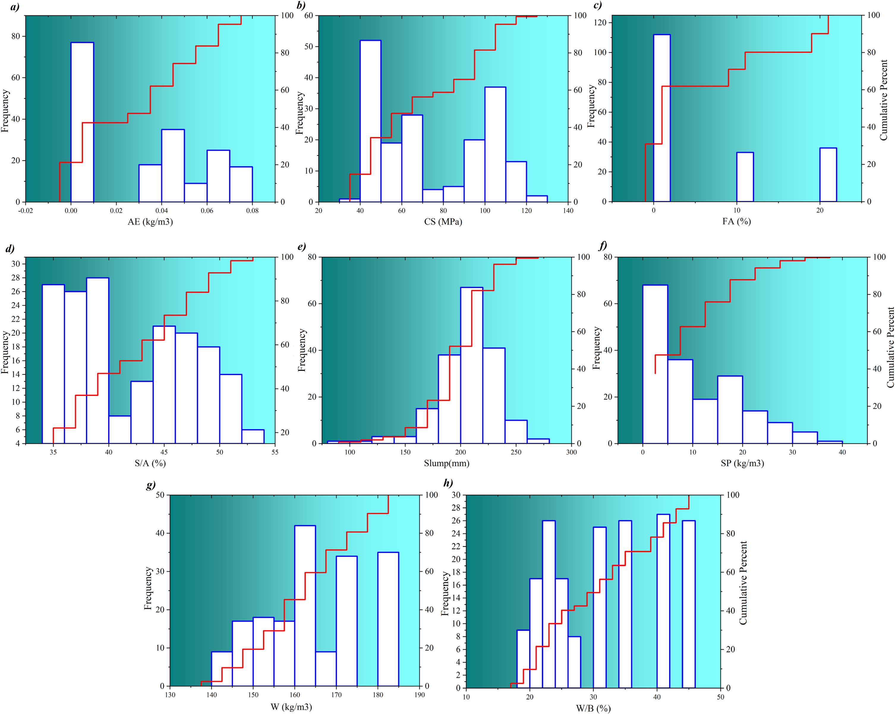
Ingredients and hardness properties of HPC compounds including a) air entering agent, b) compressive strength, c) fly-ash, d) fine to total aggregates, e) slump, f) superplasticizer, g) water content, and h) water to binder ratio.

2.2 AdaBoost (ADA)

AdaBoost is a strong approach originally suggested for predicting HPC features. Freund and Schapire [23] proposed the AdaBoost algorithm. They demonstrated that a precise “strong” learning algorithm could be acquired by adding many “weak” learning algorithms. The random guess learning algorithm is a little worse than each algorithm. Consider the input dataset is represented as: $\begin{matrix} A = {(x_{1}, y_{1}), (x_{2}, y_{2}), \dots, (x_{n}, y_{n})}, \\ y \in {- 1, + 1} \end{matrix}$ (1)

Here x shows the vector, and y indicates the target class label. AdaBoost repeatedly calls low learning algorithm or a particular weak at a time intervals’ series n = 1, 2, …, N. Each training sample is represented with the same initialized weights as: $ω_{n, i} = {\begin{matrix} \frac{1}{2 F}, y = - 1 \\ \frac{1}{2 T}, y = 1 \end{matrix}$ (2)

Here F shows the amount of, and T is the number of “true” samples. The training set received N rounds of training. The goal of training is to optimize the best classifier c_n and finds a strong classifier. This can be achieved by decreasing or increasing the weight of the classified samples after each round of training in order to focus on the hard samples in the training set. The rule for updating the weights is as follows: $R_{i + 1} (i) = \frac{R_{n} (i) . e^{- p_{i} . y_{i} . c_{i} . (x_{i})}}{L_{n}}$ (3) Here L_n shows a factor of normalization, c_i determines the base classifier, and p_i is the parameter that iteratively underrates the possibility of c_i. $L_{n} = \sum_{i = 1}^{W} R_{n} (i) . \exp (- p_{i} . y_{i} . c_{i} . (x_{i}))$ (4)

Here R_n (i) shows the training sample’s distribution weight (i) in the round [33]. Therefore, the final classifier G can be acquired by combining many elementary classifiers by weighted majority voting as expressed in Equation 5: $G (x) = sign (\sum_{i = 1}^{N} p_{i} . c_{i} (x))$ (5)

The AdaBoost framework can be sketched using Fig. 3 [33]:

Fig. 3

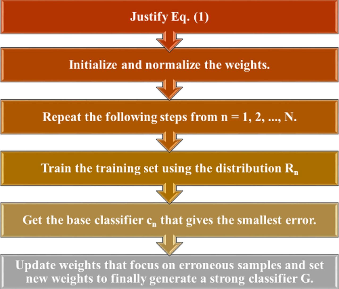
AdaBoost framework.

2.3 Decision Tree (DT)

A decision tree (DT) is generated by developing an algorithm that divides a data set (instance) into branching features. The features construct an inverse DT starting from the root node at the top of the tree. Figure 4 is indicated an example tree with five nodes and six leaves. Figure 4 determined that DT can contain both discrete and continuous attributes. Create decision rules that form branches and segments under the root node using the relationship between the analysis target, the analysis target, and the target field of the data, which is the input field. One time the relationships are configured, one or more decision rules can be emanated that represent the relationship between inputs and outputs. It can be utilized to select rules and show DT. It supplies a means of visually examining and describing the tree-like network of relationships that characterize input and output values. A decision rule predicts, with some degree of accuracy, new or invisible observations that contain the value of the input but may not have the value of the target.

Fig. 4

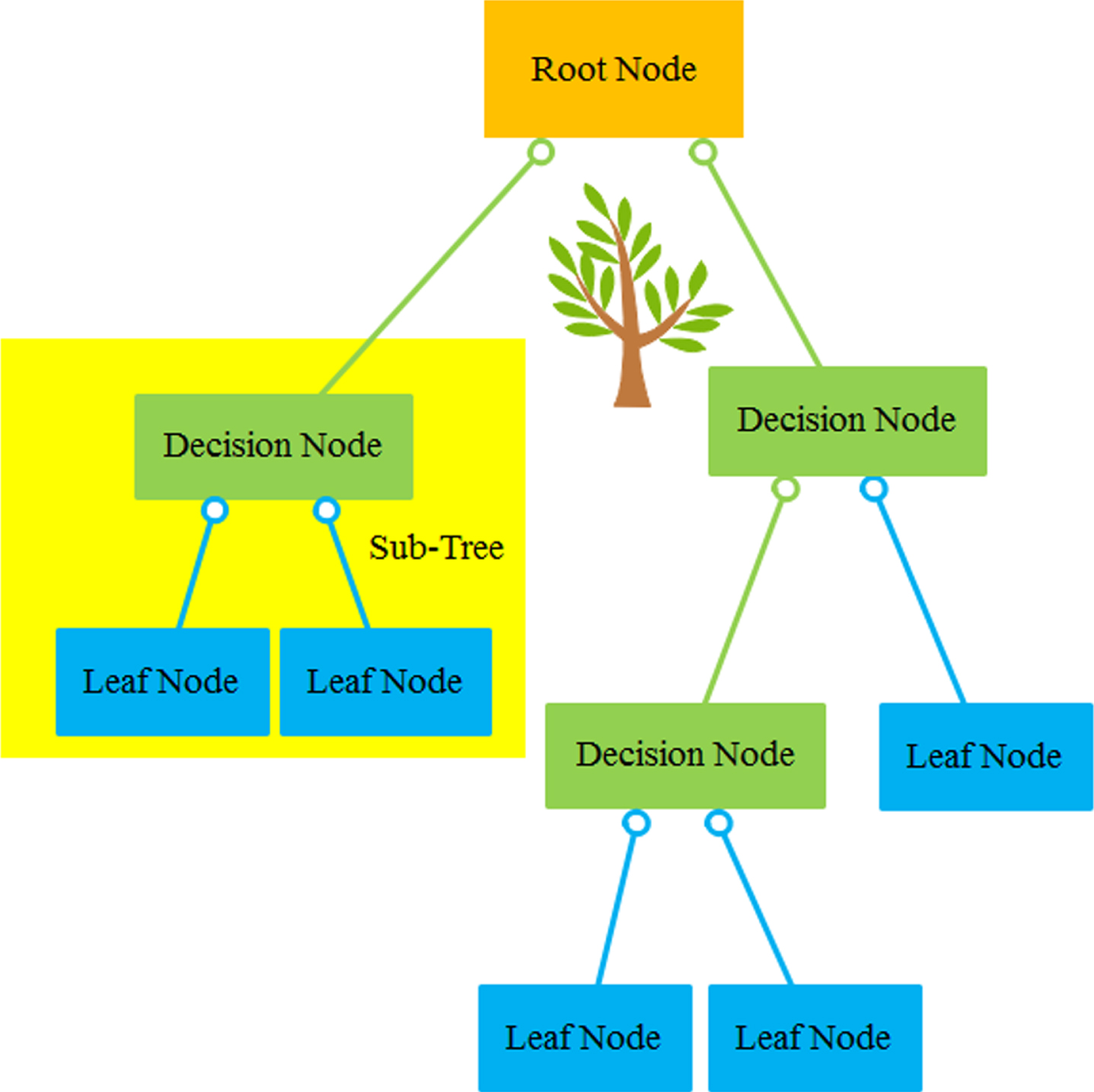
Decision Tree’s structure.

Split efficiency is computed from the entropy difference or information gain resulting from the choice of attributes for splitting the dataset. The entropy of the information of the set C for the selected attribute (the attribute on which the split is performed) is computed as: $F (C) = - \sum_{i = 1}^{N} e_{c} (k) . lo g_{2} e_{c} (k)$ (6)

Where N shows the number of distinct values for the selected attribute and e_c (k) determined the frequency of kith values for that attribute in set C. According to the description of entropy, zero entropy shows a perfectly sorted set. As a result, features with higher entropy are more likely to become shard nodes for improved classification. This is measured by calculating the profit resulting from splitting the feature, E_i. $J (C, E_{i}) = - \sum_{i = 1}^{N} e_{c} (E_{ik}) . lo g_{2} E (C_{E_{ik}})$ (7) where E_ik shows the kith value of feature E_i, e_c (E_ik) determined the frequency of models in set C with E_ik as the value of feature E_i, and C_{E
_ik} shows the subset of C consists of all instances where E_i is E_ik. Eventually, attributes with higher gain are selected as shard nodes to enhance entropy.

2.4 Support Vector Regression (SVR)

The Support Vector Machine (SVM) algorithm is a popular regression and classification technique according to statistical learning theory [34]. Support vector regression (SVR) was designed to solve regression issues with the introduction of Vapnik’s ɛ-insensitive loss function. SVR uses the principle of structural risk underestimation to enhance its conception ability even when built using a limited training data set. From the actual target for all training data, this underestimation aims to obtain a function with at most ɛ errors. Avoiding errors is unavoidable, so the goal is to hold the error within a certain range of values (ɛ). The relationship between the input and output variables of nonlinear mapping is given in the following [35]: $c (s) = (w . δ (s)) + k$ (8)

Here, s is the input value, z_i is the output value and δ (s) is an irregular function that maps the input data to a high-dimensional territory. In addition, w ∈ Rⁿ shows a weight vector that determines the discriminant plane’s orientation, k ∈ R indicates a scalar threshold that defines the displacement of the discriminant plane from the origin (i.e., the bias term), and n is the training data’s next size. Vapnik’s ɛ-insensitive loss function is expressed in the following [34]. $| y - c (s) | = \max {0, | y - c (s) | - ɛ}, ɛ > 0$ (9)

The flatness of Equation 8 relies on fewer values of w. The function cannot return an error smaller than ɛ for every data point. To allow for more errors, slack variables $ξ_{i}, ξ_{i}^{*}$ are presented. Therefore, the optimization function can be determined in SVR in the following [34]: $\begin{matrix} Min : \frac{1}{2} ∥ w^{2} ∥ K \sum_{i = 1}^{N} (ξ_{i} - ξ_{i}^{*}) \\ Subject o : {\begin{matrix} z_{i} - (w . δ (s)) + k \leq ɛ + ξ_{j} \\ (w . δ (s)) + k - z_{i} \leq ɛ + \underset{j}{ξ^{*}} \\ ξ_{j}, \underset{j}{ξ^{*}} \geq 0 \end{matrix} \end{matrix}$ (10)

Here k shows a regularization constant determined as the correction characteristic of exhibiting the trade-off between the flatness of the model and the practical error. The slack variables are zero for all data points within the progressive increase and the ɛ-insensitive zone for data points outside the zone. The solution to the optimization problem explained via Smola and Scholkopf [36] which in Equation (10) by converting it into a dual formulation using Lagrange multipliers $η_{i}, η_{i}^{*}, α_{i}, α_{i}^{*}$ . The final form of the solution can be given as: $\begin{matrix} \max {\begin{matrix} \frac{1}{2} \sum_{j, i = 1}^{n} (a_{j} - a_{j}^{*}) (a_{i} - a_{i}^{*}) C (s_{j}, s_{i}) \\ - ɛ \sum_{j = 1}^{n} (a_{j} - a_{j}^{*}) + \sum_{j = 1}^{n} y_{j} (a_{j} - a_{j}^{*}) \end{matrix} \\ the \sum_{j = 1}^{n} (a_{j} - a_{j}^{*}) = 0; 0 a_{j}, a_{j}^{*} \leq T \end{matrix}$ (11)

Here C (s_j, s_i) is determined as the kernel function

Then solving Equation 11 for the $a_{j}, a_{j}^{*}$ value. $c (s) = \sum_{j, i = 1}^{n} (a_{i} - a_{i}^{*}) C (s_{j}, s_{i}) + k$ (12)

A kernel function is computed instead of φ(z) to decrease the complexity of high-dimensional attribute space processing in the optimization problem. Kernel functions widely utilized in regression contain polynomial kernel functions, linear kernel functions, sigmoid kernel functions, and radial basis functions (RBF). The following RBF is used considering the infinite-dimensional feature space corresponding to the RBF. $C (s_{j}, s_{i}) = e^{(- y ∥ s_{j} - {s_{i}}^{2} ∥)}$ (13)

Here $γ = \frac{1}{σ^{2}}$ shows the parameter of RBF.

In the present article, optimized structure of SVR model should be considered as the main aim. In this regard, working process of SVR requires to be regulated with some external tools that are defined in next sections. Determining internal parameters’ values of SVR as arbitrary values is an optimizing task to be done with optimization algorithm. The parameters to optimize the working process of main model are ξ, ɛ and K.

2.5 Chaos game optimizer (CGO)

Based on the presented chaos theory principles, an optimization algorithm is proposed. Formulate a mathematical model for CGO algorithms using the basic concepts of fractal and chaotic game theory. To this end, due to the fact that many natural evolutionary algorithms maintain a solutions’ population that evolves by random changes and selections, the CGO algorithm uses a series of points representing some suitable point in the Sierpinski triangle to consider candidate solutions (X). Each candidate solution (X_i) includes some decision variables (x_i,j) Representing the positions of eligible points within the Sierpinski triangle in this algorithm. The optimization algorithm uses the Sierpinski triangle as a search space for candidate solutions. The mathematical representations of these aspects are: $X = [\begin{matrix} X_{1} \\ X_{2} \\ ⋮ \\ X_{n} \end{matrix}] = [\begin{matrix} x_{1}^{1} \\ x_{2}^{1} \\ \dots \\ x_{n}^{1} \end{matrix} \begin{matrix} x_{1}^{2} \\ x_{2}^{2} \\ \dots \\ x_{n}^{2} \end{matrix} \begin{matrix} \dots \\ \dots \\ ⋱ \\ \dots \end{matrix} \begin{matrix} x_{1}^{d} \\ x_{2}^{d} \\ ⋮ \\ x_{n}^{d} \end{matrix}]$ (14)

Here n shows the acceptable points’ number in the Sierpinski triangle, and d indicates these points’ dimensions.

The first positions of suitable points to be considered are defined randomly in the explore space in the following: $x_{i}^{j} (0) = x_{i, \min}^{j} + rand \times (x_{i, \max}^{j} - x_{i, \min}^{j}), {\begin{matrix} i = 1, 2, \dots, n . \\ j = 1, 2, \dots, d . \end{matrix}$ (15) }

Here $x_{i}^{j} (0)$ defines the eligible point’s starting position. $x_{i, \max}^{j}$ and $x_{i, \min}^{j}$ show the maximum and minimum tolerances for the j^th decision variable of the i^th solution candidate. rand shows a random number in the [0,1] interval.

The main idea of this mathematical model is to generate various suitable points in the explore space to complete the Sierpinski triangle’s general shape. Furthermore, the method of creating new points within the Sierpinski triangle, as explained in Fig. 5, is used for this suggestion. To the first suitable of each point in the explore space (X_i), a temporary triangle is considered and drawn in three points in the following:

So far found the Global Best (GB) position,

The i^th solution candidate (X_i) is the chosen first eligible point position

GB apply to the candidate optimal solution with the highest fitness level found so far, and MGi are some randomly chosen first qualifying points with equal probability of containing the currently considered first eligible point (X_i).

The MGi and GB next to the first eligible point chosen (X_i) are taken to be the Sierpinski triangle’s three vertices. Figure 6 indicates a schematic diagram of temporary triangle creation. Figure 7 also illustrates a more detailed schematic description of this aspect.

Fig. 5

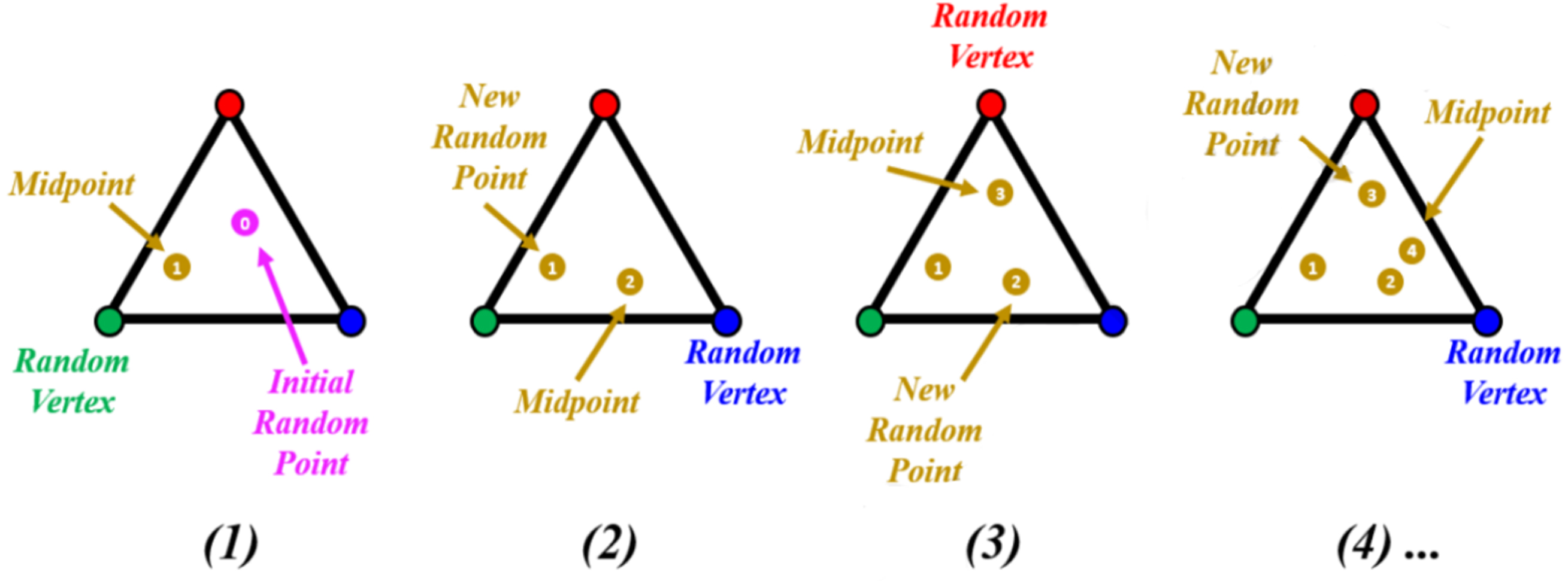
A chaos game methodology for creating Sierpinski triangles [31].

Fig. 6

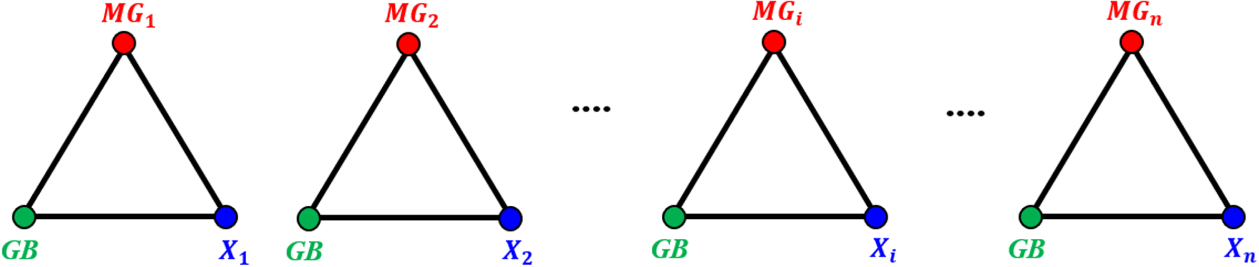
Schematic for creating temporary triangles [31].

Fig. 7

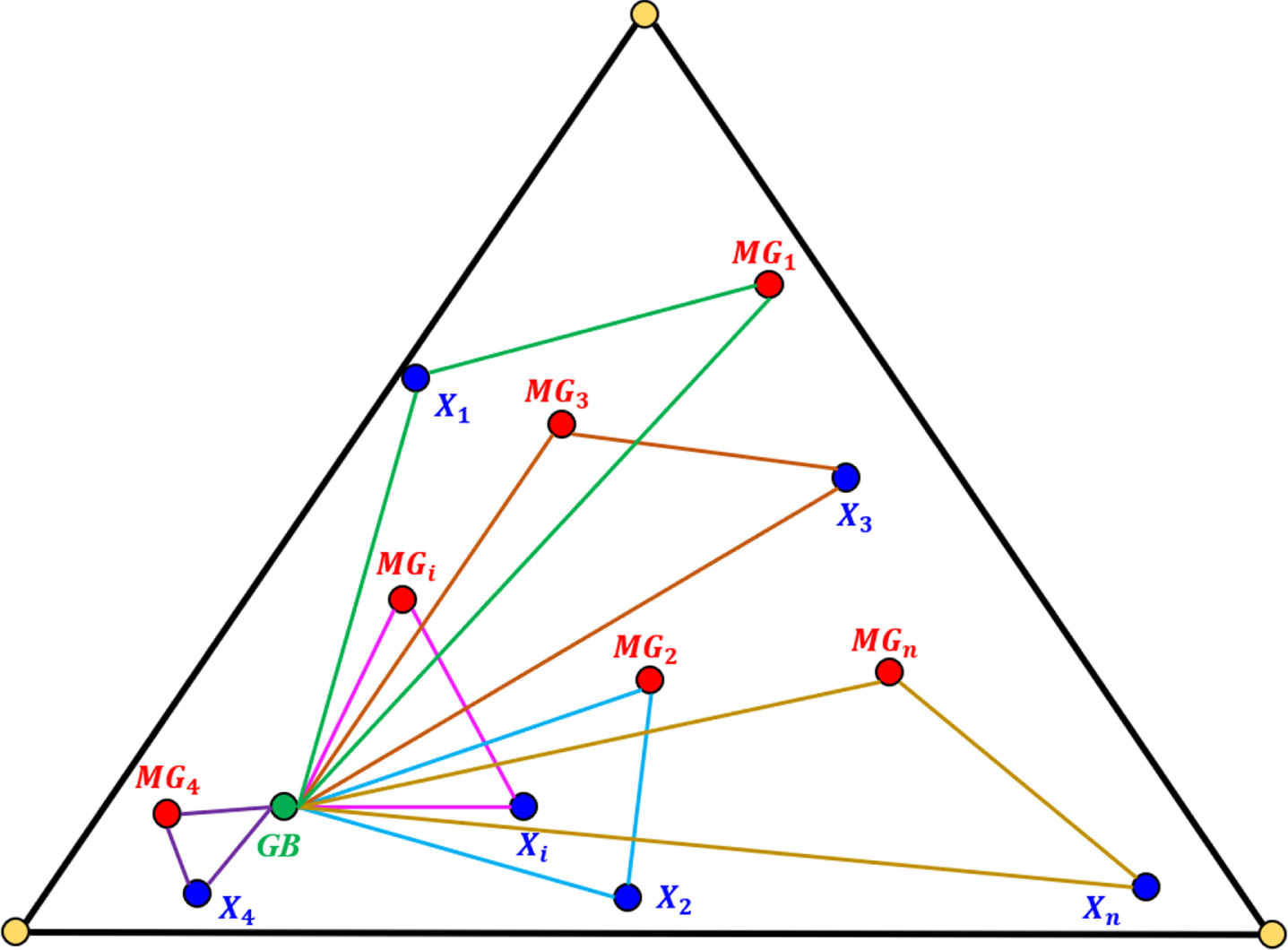
Schematic representation of a temporary triangle in the search space [31].

Some randomly developed factors are also used because the chaos game methodology to control the aspect requires constraining the movement of seeds within the explore space. To this end, some randomly generated factors have been used to control this aspect, based on the fact that the chaos game methodology requires us to constrain the action of the seed within the explore space. This process’s mathematical representation is: $S_{i}^{j} = X_{i} + a_{i} \times (b_{i} \times GB - c_{i} \times M G_{i}), i = 1, 2, \dots, n .$ (16) }

Here X_i shows the i^th solution candidate, G_B indicates the global best found so far, and MGi shows the mean of some primary suitable point values to be considered the 3 vertices of the ith temporal triangle. ai shows a randomly developed factorial utilized to model motion limits. The seeds, b_i and c_i, describe random integers of 0 or 1 to model a chance to roll the die, respectively.

To control and tune the search and utilization of the suggested new CGO algorithm, 4 different equations are used to determine a_i, which is related to modeling the action constraint of seeds. These equations are randomly used in each of Equation 16, where the positions of the first through third seeds are defined as follows: $a_{i} = {\begin{matrix} Rand \\ 2 \times Rand \\ (μ \times Rand) + 1 \\ (θ \times Rand) \end{matrix}$ (17)

Here Rand shows a uniformly distributed random number on the interval [0,1], and μ and θ define random numbers on the interval [0,1]

2.6 Preparing ensemble and hybrid models

The ensemble method organizes the above model sets according to their combination and performance of the highest performing models into an ensemble model. The ensemble process can be mathematically defined as $y : ℝ^{d \to} ℝ$ with a d-dimensional estimator variable X and a d-dimensional answer Y. Each process obtains a predicted function y (x) utilizing the specified algorithm. The estimated set-based function y_en (x) is achieved from a linear combination of the single function: $y_{en} (x) = \sum_{i = 1}^{N} s_{i} \times y (x)$ (18)

Based on Equation 18, s_i primary containing linear combination coefficients depending on the average of the different weights. Accordingly, this article gathered three models of AdaBoost, Decision Tree, and Support Vector Regression in a holistic SDA framework.

In addition, developing hybrid frameworks requires optimizing estimative models with regard to internal settings. For example, in this study, SVR contains some arbitrary variables because model fits are optimized with the aid of the three parameters ɛ, ξ, and K. By combining SVR, ADA, and DT with CGO, three hybrid models SVGO, ADGO, and DTGO were developed. Figure 8 illustrates designing the hybrid and ensemble models.

Fig. 8

A schematic view of developing ensemble and hybrid frameworks.

2.7 Performance evaluation methods

The article evaluates the predictive accuracy of DT-ADA-SVR, DT-CGO, ADA-CGO, and SVR-CGO models employing correlation coefficient (R²), mean absolute error (MAE), and root means squared error (RMSE), variance account factor (VAF), and objective detection metrics (OBJ). These statistical evaluators are expressed in the following: $R^{2} = {(\frac{\sum_{i = 1}^{n} (p_{i} - \bar{p}) (r_{i} - \bar{r})}{\sqrt{[\sum_{i = 1}^{n} {(p_{i} - p)}^{2}] [\sum_{i = 1}^{n} {(r_{i} - \bar{r})}^{2}]}})}^{2}$ (19) $RMSE = \sqrt{\frac{1}{n} \sum_{i = 1}^{n} {(r_{i} - p_{i})}^{2}}$ (20) $MAE = \frac{1}{n} \sum_{i = 1}^{n} | r_{i} - p_{i} |$ (21) $VAF = (1 - \frac{var (t_{n} - e_{n})}{var (t_{n})}) \times 100$ (22)

$\begin{matrix} OBJ = (\frac{t_{train} - t_{test}}{e t_{train} + t_{test}}) \frac{MA E_{test} + RMS E_{train}}{1 + R_{train}^{2}} \\ + (\frac{2 t_{train}}{t_{test} + t_{train}}) \frac{RMS E_{test} - MA E_{test}}{1 + R_{test}^{2}} \end{matrix}$ (23)

Alternatively, p and r are the experimental and predicted Slump and CS values. n shows the data instances’ number, $\bar{p}$ determined the average experimental Slump and CS value, and $\bar{r}$ defined the average predicted Slump and CS value.

A k-fold cross-validation procedure is often utilized to decrease the bias of randomly splitting a data set into training and testing sets. The dataset is divided into k partitions (k = 5 or k = 10) in k-fold cross-validation. a fold is the name of each partition of data. One fold is employed for model testing, and the remaining k-1 folds are utilized for model training. The strategy is repeated k times with a different test set. Then performing cross-validation, the standard deviation and mean of the key performance indicators are calculated.

3 Results and discussion

The data employed in this paper included 189 residual slump and compressive strength experimental results from previously published syntheses [32]. It should be noted that the sample selected from the cited article was taken at 28 days of age. In the paper, alternatively, 70% and 30% of samples were collected for training and testing the proposed model. Statistical consistency of data sets for training and testing optimizes model performance and ultimately improves model analysis.

Table 1 shows the results of the models considered to evaluate their accuracy. In the table of models in the sections of training, validation, testing, and all data on compressive strength and slump flow have been examined. The evaluators introduced in the previous section compare the models based on the highest and lowest value, except for R² and VAF, the lowest value of the other evaluators indicates proper performance. In the section related to compressive strength, the performance of the models is as follows:

Table 1
The results of the models are considered to evaluate their accuracy.

HPC Model Modeling Index values

Feature name phase R² RMSE MAE VAF OBJ

SVGO Train 0.9741 4.246 3.4417 99.111 4.626

Validation 0.9726 4.3649 3.4594 98.927

Test 0.9876 3.1776 2.6737 99.572

All 0.9757 4.1187 3.3265 99.156

DTGO Train 0.9684 4.7041 2.8561 98.047 5.514

Validation 0.9733 4.363 3.0357 98.513

Test 0.9843 3.4591 2.5172 99.184

All 0.9716 4.4845 2.8307 98.269

ADGO Train 0.996 1.572 1.165 99.840 5.480

Compressive strength Validation 0.993 2.242 1.832 99.747

Test 0.999 0.876 0.662 99.952

All 0.996 1.609 1.187 99.831

SDA Train 0.985 4.561 3.223 98.477 3.194

Validation 0.987 3.945 3.137 99.134

Test 0.990 3.144 2.460 99.444

All 0.984 4.284 3.093 98.744

SVGO Train 0.933 7.175 5.663 97.429 6.688

Validation 0.870 8.254 6.588 94.670

Test 0.889 6.826 5.931 97.043

All 0.920 7.294 5.841 97.099

DTGO Train 0.888 9.329 7.294 95.536 7.421

Validation 0.888 7.298 6.775 98.416

Test 0.897 6.852 6.074 97.394

All 0.888 8.711 7.030 95.978

ADGO Train 0.922 7.805 6.472 97.480 3.046

Slump flow Validation 0.841 8.593 7.375 95.808

Test 0.766 9.818 7.929 91.314

All 0.899 8.263 6.829 96.710

SDA Train 0.968 5.157 3.971 98.595 2.375

Validation 0.944 5.326 3.531 96.575

Test 0.931 5.293 3.716 96.320

All 0.961 5.204 3.867 98.156

HPC	Model	Modeling	Index values
	SVGO	Train	0.9741	4.246	3.4417	99.111	4.626
		Validation	0.9726	4.3649	3.4594	98.927
		Test	0.9876	3.1776	2.6737	99.572
		All	0.9757	4.1187	3.3265	99.156
	DTGO	Train	0.9684	4.7041	2.8561	98.047	5.514
		Validation	0.9733	4.363	3.0357	98.513
		Test	0.9843	3.4591	2.5172	99.184
		All	0.9716	4.4845	2.8307	98.269
	ADGO	Train	0.996	1.572	1.165	99.840	5.480
Compressive strength		Validation	0.993	2.242	1.832	99.747
		Test	0.999	0.876	0.662	99.952
		All	0.996	1.609	1.187	99.831
	SDA	Train	0.985	4.561	3.223	98.477	3.194
		Validation	0.987	3.945	3.137	99.134
		Test	0.990	3.144	2.460	99.444
		All	0.984	4.284	3.093	98.744
	SVGO	Train	0.933	7.175	5.663	97.429	6.688
		Validation	0.870	8.254	6.588	94.670
		Test	0.889	6.826	5.931	97.043
		All	0.920	7.294	5.841	97.099
	DTGO	Train	0.888	9.329	7.294	95.536	7.421
		Validation	0.888	7.298	6.775	98.416
		Test	0.897	6.852	6.074	97.394
		All	0.888	8.711	7.030	95.978
	ADGO	Train	0.922	7.805	6.472	97.480	3.046
Slump flow		Validation	0.841	8.593	7.375	95.808
		Test	0.766	9.818	7.929	91.314
		All	0.899	8.263	6.829	96.710
	SDA	Train	0.968	5.157	3.971	98.595	2.375
		Validation	0.944	5.326	3.531	96.575
		Test	0.931	5.293	3.716	96.320
		All	0.961	5.204	3.867	98.156

The hybrid ADGO model for R² was able to obtain the highest value equal to 0.996, so its difference with DTGO and SVGO was 2%. Also, compared to the ensemble model, SDA has been able to perform better, with a difference of 1%.

The next evaluation, which is related to RMSE and the most acceptable performance, is still ADGO which has a value equal to 1.609, which is a remarkable value compared to other models. ADGO has a difference of 61% with SVGO, and this difference with DTGO equals 64%. In addition, the RMSE of SDA is equal to 4.284, and its difference from ADGO is 62%.

MAE, which is another model error descriptor. Like the previous evaluators, in this evaluator, the lowest value, equal to 1.187, belonged to ADGO. Comparing the model with the rest of the models, the values of SVGO and DTGO are equal to 3.3265 and 2.8307, and their difference with ADGO is 64% and 58%, respectively. Moreover, it has performed well compared to SDA, which has registered a difference of 62.

The value of VAF, like R², must be the highest. The performance of the models in the respective evaluation set is almost the same. But in general, ADGO has the highest value, equal to 99,831. Compared to DTGO, whose performance is as low as 98.269, they have a 1.5% difference. This difference indicates that all models function correctly in the VAF evaluator.

The last evaluator that should have the lowest value is OBJ. Unlike the other evaluators, ADGO performed better than the others. In OBJ, the SDA ensemble model had the lowest value of 3.194. In expressing the difference between the models and SDA, SVGO, DTGO, and ADGO are 31, 42, and 41%, respectively.

In Slump flow, the performance of combined and ensemble models has been obtained as follows:

The SDA ensemble model for R² can achieve the highest value of 0.961, so the difference between DTGO and SVGO is 8 and 4 percent, respectively. Also, compared to the ADGO, the SDA was able to outperform with a margin of 6%.

The next evaluation regarding RMSE and the most accepted performance is SDA, with a value of 5.204 which is a unique value compared to other models. SDA has a spread with SVGO of 28% and this difference with DTGO of 40%. Furthermore, ADGO’s RMSE equals 8.263, and its difference with SDA is 36%.

Another error descriptor is MAE. As with the previous evaluator, the lowest value equal to 3.867 belonged to SDA for this evaluator. Comparing the model with the rest, the values for SVGO and DTGO are equal to 5.841 and 7.03, with differences from SDA of 34% and 45%, alternatively. It also performs suitable when compared to the ADGO, which had a difference of 43%.

In the VAF evaluator, the ensemble model, SDA, has obtained the highest value. Meanwhile, DTGO has obtained the lowest value among all models. Of course, it should be noted that the difference between SDA and the rest of the models was not more than 2%, and this indicates that the models performed closely with each other in obtaining the VAF value.

In OBJ, the SDA set model can have a value as low as 2.375, representing the difference between SDA and other models; SVGO, DTGO, and ADGO are 64, 68, and 22 percent, alternatively.

In general, it can be stated that in the compressive strength of the ADGO composite model, it had a stronger performance, and DTGO had the weakest performance. On the other hand, SDA obtained the most suitable values for slump flow, and DTGO obtained the poorest values in a slump.

Figure 9 shows the measured and predicted CS based on the scatter plot. The scatters are defined as a function of RMSE and R². R² has the role of placing the sample point on the X = Y line. The RMSE feature also indicates the dispersion of the scatters, so the lower value of the component has the lower dispersion and inverse. As mentioned, the other points are directly related to the component and should have low and high RMSE and R² values alternatively. Comparing the two hybrid models identifies SVGO and DTGO, as shown in Fig. 9-a and 9-b. The points behave similarly due to the two models are close in value. Figure 9-c and 9-d illustrate the hybrid and ensemble models called ADGO and SDA, respectively. The biggest difference between these two models is the RMSE, which shows the dispersion. Figure 9-c, related to ADGO, has a lower RMSE, is close to 1, and therefore has much lower dispersion. In general, ADGO was able to have a better display in Fig. 9.

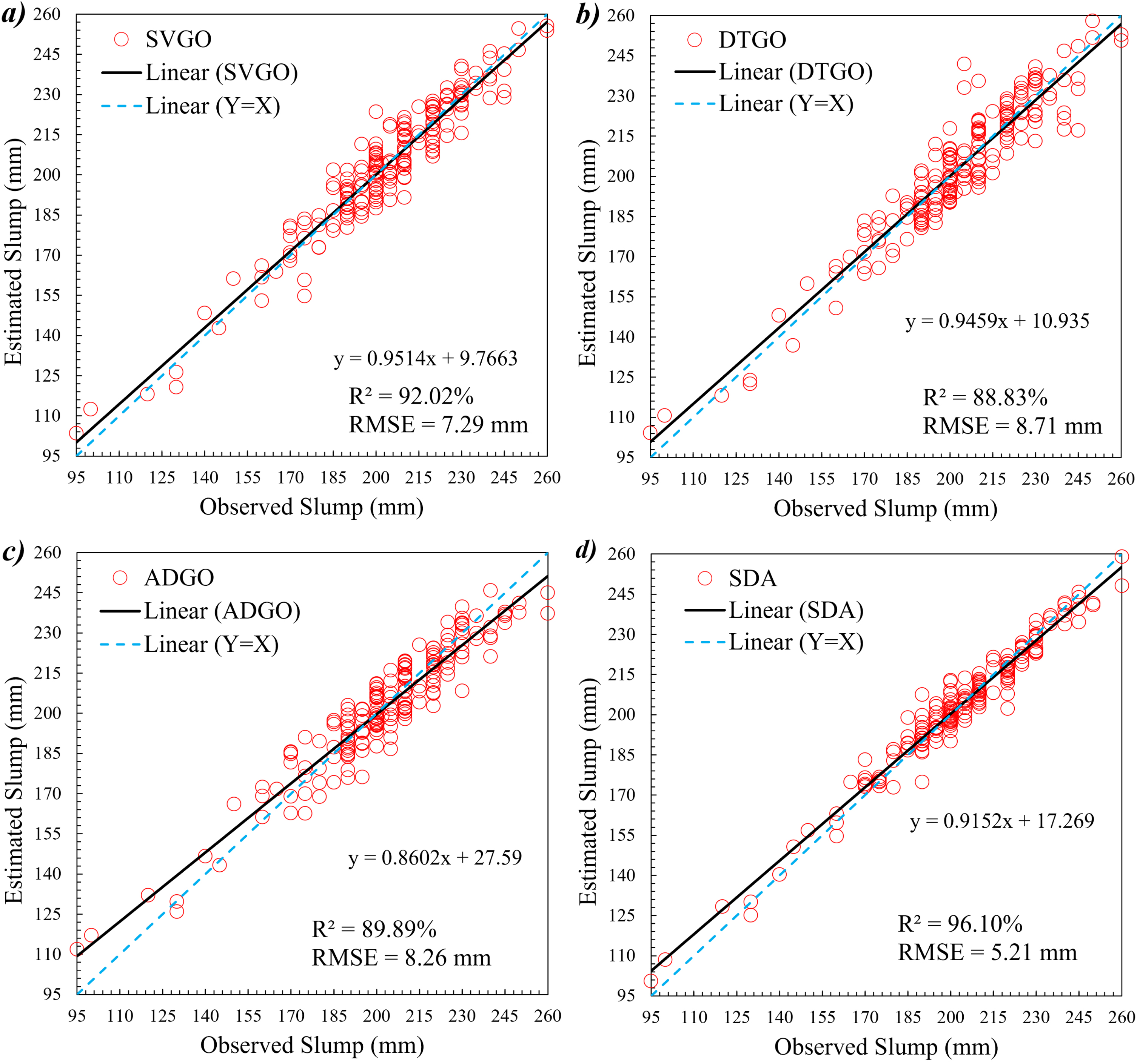
Figure 10 relates to Slump and is like the description of Fig. 9. Comparing the combined models. It can be seen that SVGO performed better than the others. But it should be noted that R² and RMSE in the models are far from 1. As a result, they do not show acceptable performance. On the other hand, SDA has better values than hybrid models. For this purpose, in general, it can be stated that this type of SDA modeling in Slump has been able to have a more suitable performance.

Fig. 9

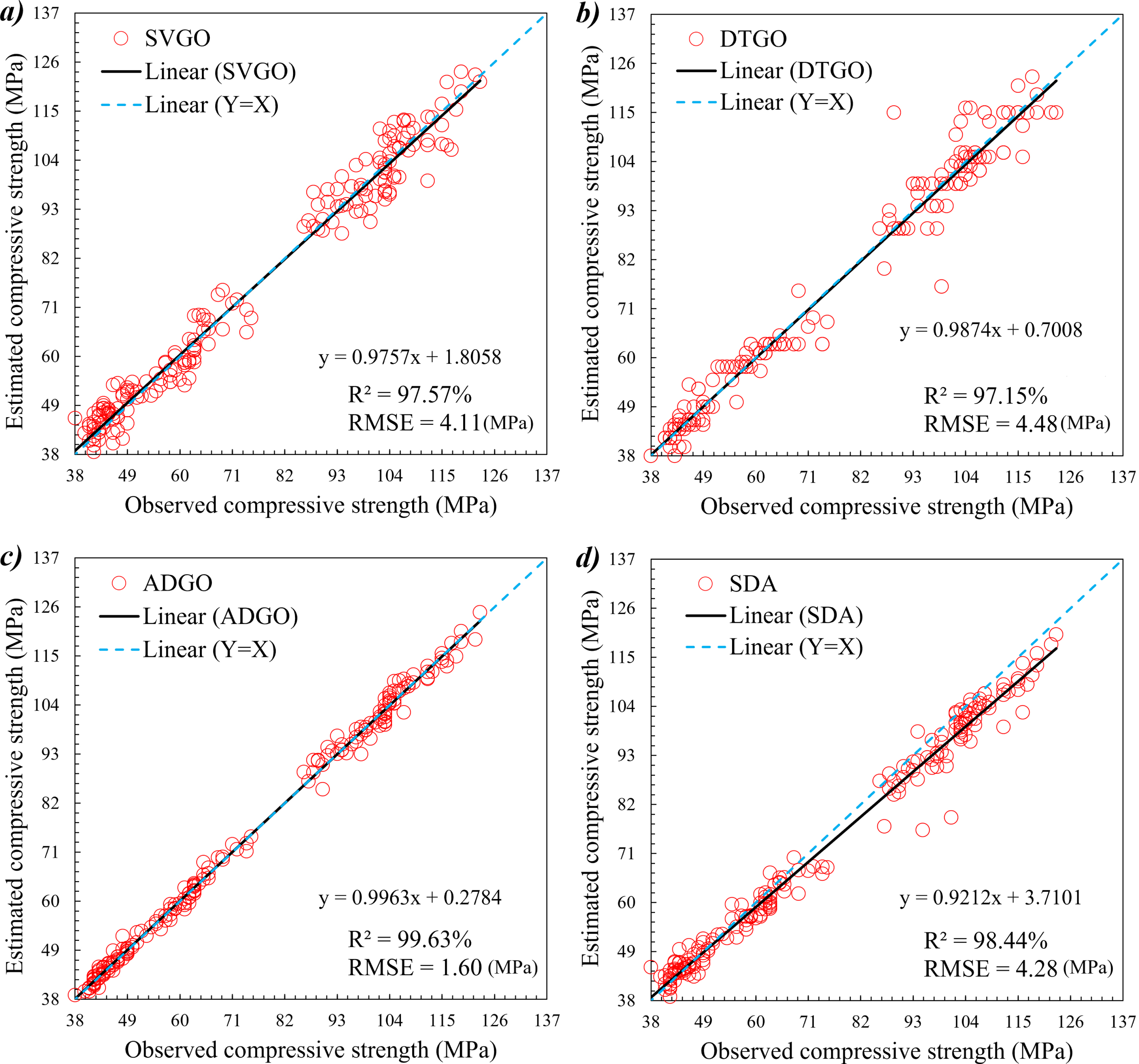
The observed and estimated compressive strength based on the scatter plot.

Fig. 10

The measured and predicted compressive strength based on the scatter plot.

Figure 11 shows the comparison line plot of predicted and measured CS during the training and testing phases. The chart contains two predicted lines and a measurement line. The detection approach is that the predicted point lies on the measured line. If the prediction line is higher and lower than the measured value, the sample alternates between overestimation and underestimation, respectively. There are 189 samples, of which 30% belong to the testing, and 70% belong to the training phase. Figure 11-a and 11-b are for SVGO and DTGO, alternatively. Both models have overestimation and underestimation in some samples. To better understand this issue, in the sample of 25, SVGO is overestimated, and DTGO is underestimated. Figure 11-c belongs to the ADGO hybrid model. The figure shows that the predicted lines are mostly on the measured points, and the sample is suitable and satisfactory. On the other hand, Fig. 11-d is related to SDA, which performed much weaker than ADGO but stronger than DTGO and SVGO. It can be concluded that the ADGO hybrid model has been able to perform more suitably in this type of modeling. Generally, the performance of ADGO looks to simulate the compressive strength magnitudes better than other models while some points have deviations compared to measured CS line. For example, point 9 has 3% bias and for sample 121 the error rate is calculated –5%.

Fig. 11

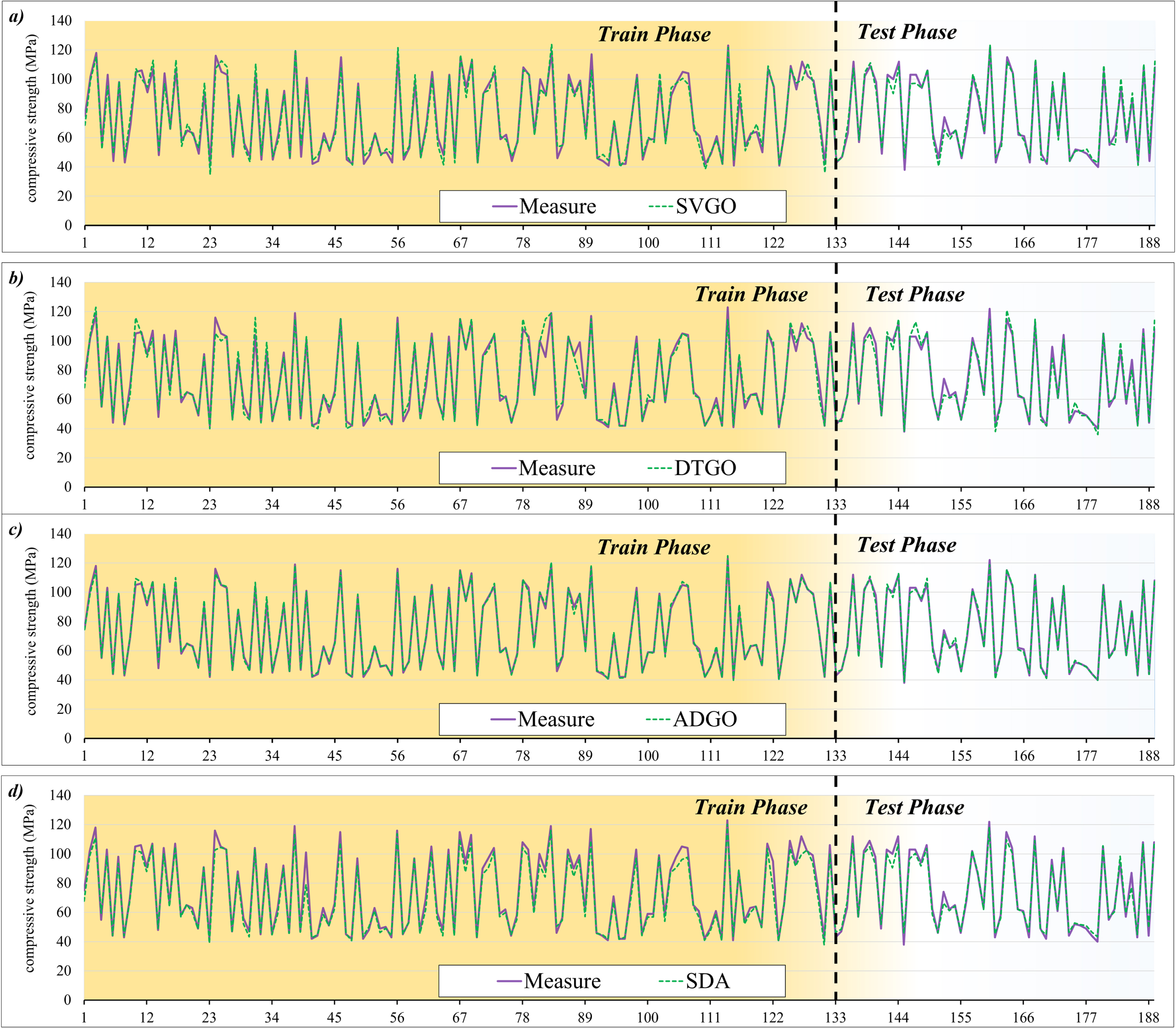
The comparison line plot of predicted and measured compressive strength.

Figure 12 shows the line plot of the predicted and measured Slump. The explanations given about the behavior and type of persuasion modeling in Fig. 11 also apply to Fig. 12. As seen from the figure, all three hybrid models have almost the same and not a very good performance, as is evident in several examples of overestimation and underestimation. But it can be mentioned that these models minimized the difference between the measured and predicted in the test phase compared to the training phase. This case shows that the models have been able to improve their performance in the test phase. On the other hand, SDA has been able to perform more satisfactorily than the hybrid models, so the difference between the lines is small, and also, in the test phase, most of the predicted lines are on the measured ones. In general, it can be said that SDA has been able to perform better than other models.

Fig. 12

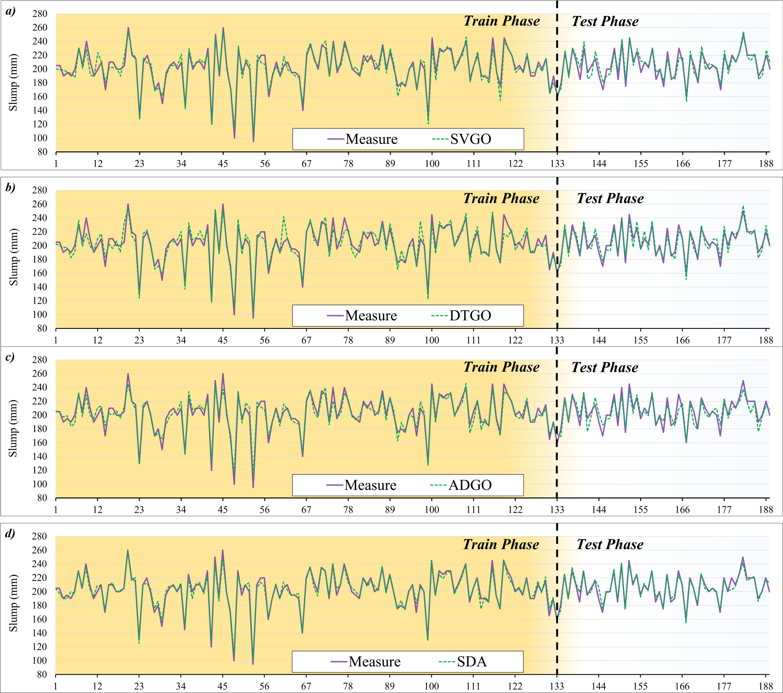
The line plot of the predicted and measured the Slump.

Figure 13 demonstrates the Taylor diagram of present models of CS and Slump. Figure 13 consists of the standard deviations and correlation coefficients (R2). The standard deviation ranges from 0 to 32, and the correlation coefficient ranges from -1 to 1. Also, the reference is indicated by a black dot in the figure, which the closer model point to the reference determines the more satisfactory models’ performance. As shown, Fig. 13-a and 13-b relate to CS and SL. In Fig. 13-a, the hybrid SVPS ADGO is the nearest to the reference, which means it has a close correlation coefficient and standard deviation value compared to the reference. In the other part, related to Fig. 13-b, the models have not shown better performance like CS. But in general, as shown in the figure, SDA has had a relatively more acceptable performance than other models.

Figure 14 shows the error percentage of compressive strength. Errors are checked in two phases, training, and testing. Figure 14-a is related to SVGO, the highest error in the training phase was approximately 19%, which increased to 25% in the test phase. Figure 14-b indicates DTGO that the maximum error was equal to 31% in the training phase, and in the testing phase, the error percentage improved and decreased to 15%. The fact that the performance improves in the test phase indicates that the model has worked better with the samples in the training phase, and the samples perform better in the test. Figure 14-c introduces ADGO, and the highest error percentage was obtained in the training and testing phase, 10 and 8, respectively. The last model, related to SDA, has obtained a maximum error of approximately 20% in both the training and testing phases. The most suitable performance belongs to ADGO, which has the strongest performance compared to other models.

Figure 15 indicates the error percentage of the Slump. Figure 15-a is for SVGO, where the maximum error in the training phase was around 13% and decreased to 10% in the testing phase. Figure 15-b represents DTGO with a maximum error equal to 19% in the training phase and an improved error percentage in the testing phase, reduced to 5%. Figure 15-c shows are for ADGO, which has the highest percentage errors of 18 and 9 in the training and testing phases. The last model associated with SDA achieved a maximum error of about 20% in both the training and testing phases. Optimal performance belongs to ADGO and is more suitable than another model.

Figure 16 shows the histogram of developed models for CS and Slump. Figure 16-a to 16-dbelong to CS, and Fig. 16-e to 16-h belong to Slump. Figure 16-a shows the performance related to the SVGO model, which shows the frequency of most samples in the range of -8 to 8 and has obtained a relatively sharp normal distribution. Figure 14-b, which is related to DTGO, has a flat normal distribution, and the abundance of the sample is in the form of a scatter. Figure 16-c belongs to the next hybrid model, that is, ADGO, where the frequency of samples is close to zero and has a sharp normal distribution. Figure 16-d shows SDA, which has almost the same performance as ADGO and a frequency close to zero and normal sharpness distribution. Among the models related to CS, it can be concluded that ADGO has been able to perform better.

On the other hand, the models related to Slump can be seen. In general, it can be said that the most suitable performance is in Fig. 16-h and related to SDA, so the highest frequency of samples is close to zero percent error and has a sharp normal distribution. In addition, the weakest performance in the Slump is related to Fig. 16-h in such a way that the samples are scattered and have a flat normal distribution.

Fig. 13

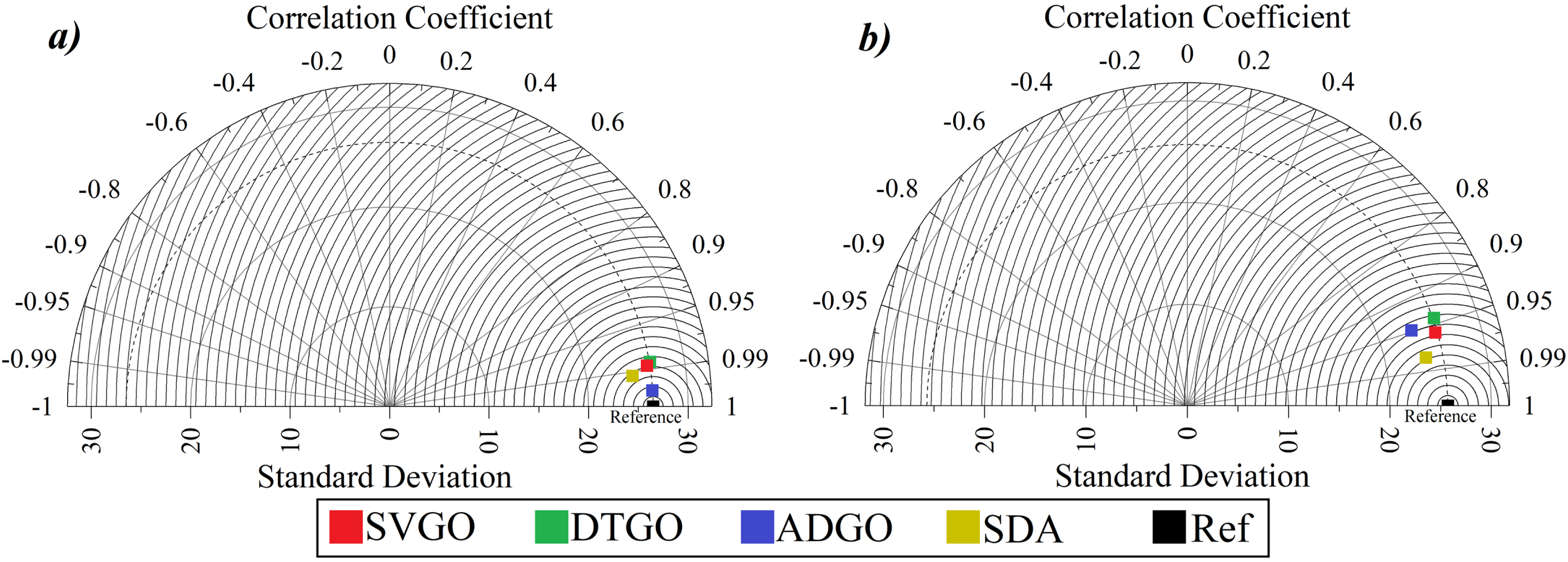
The Taylor diagram of present models of a) compressive strength and b) slump.

Fig. 14

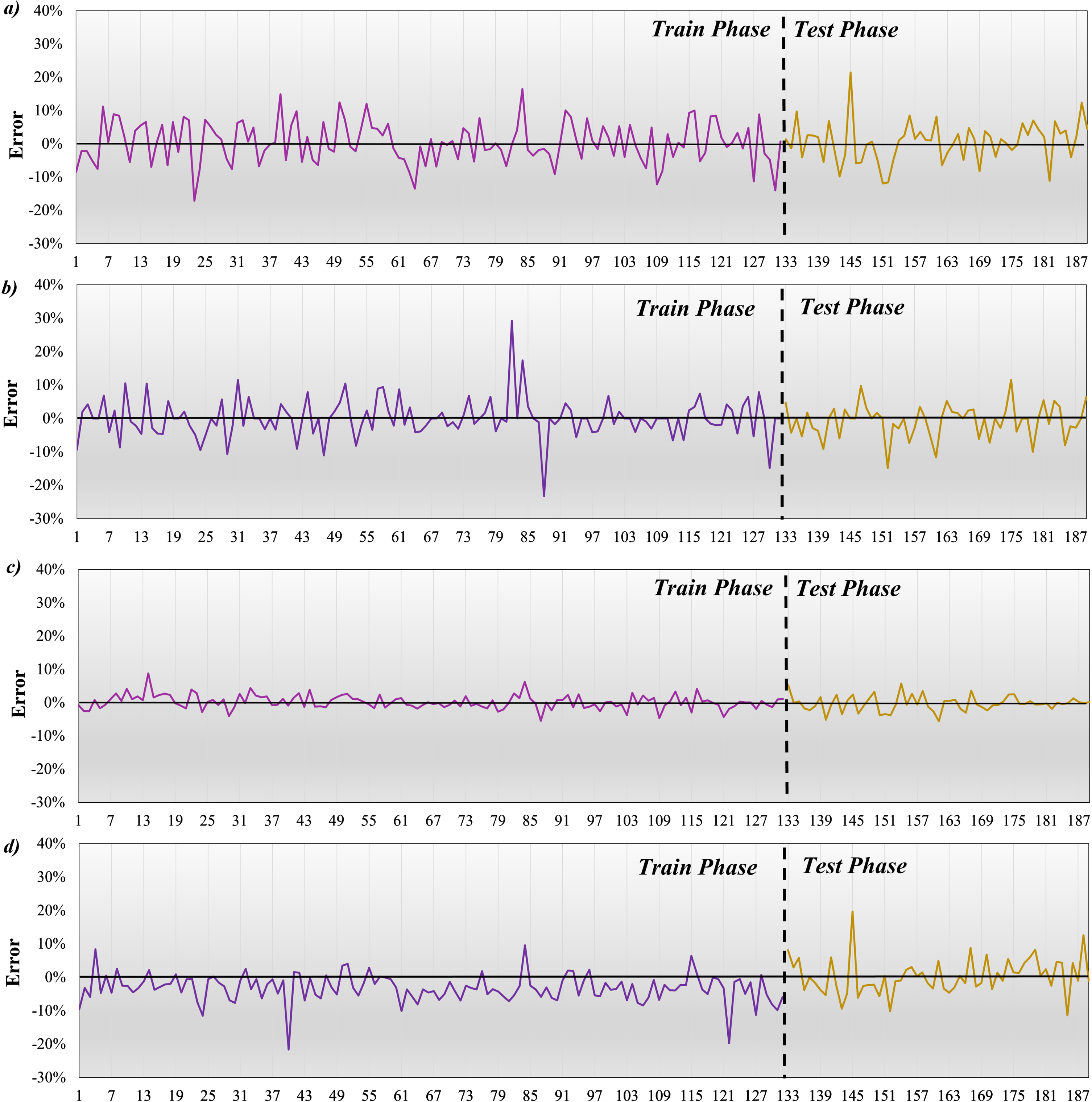
The error percentage of compressive strength a) SVGO, b) DTGO, c) ADGO, and d) SDA.

Fig. 15

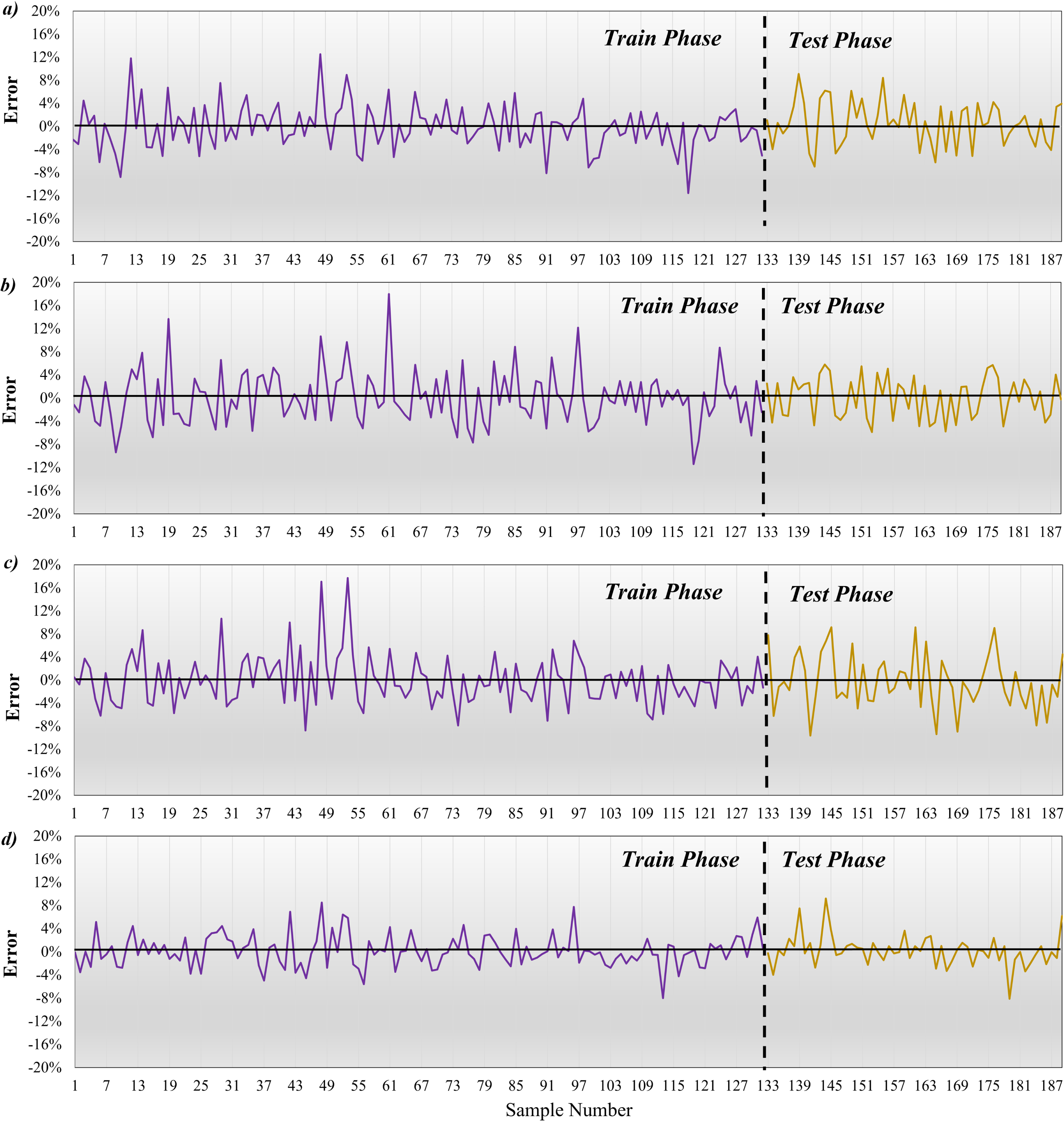
The error percentage of Slump a) SVGO, b) DTGO, c) ADGO, and d) SDA.

Fig. 16

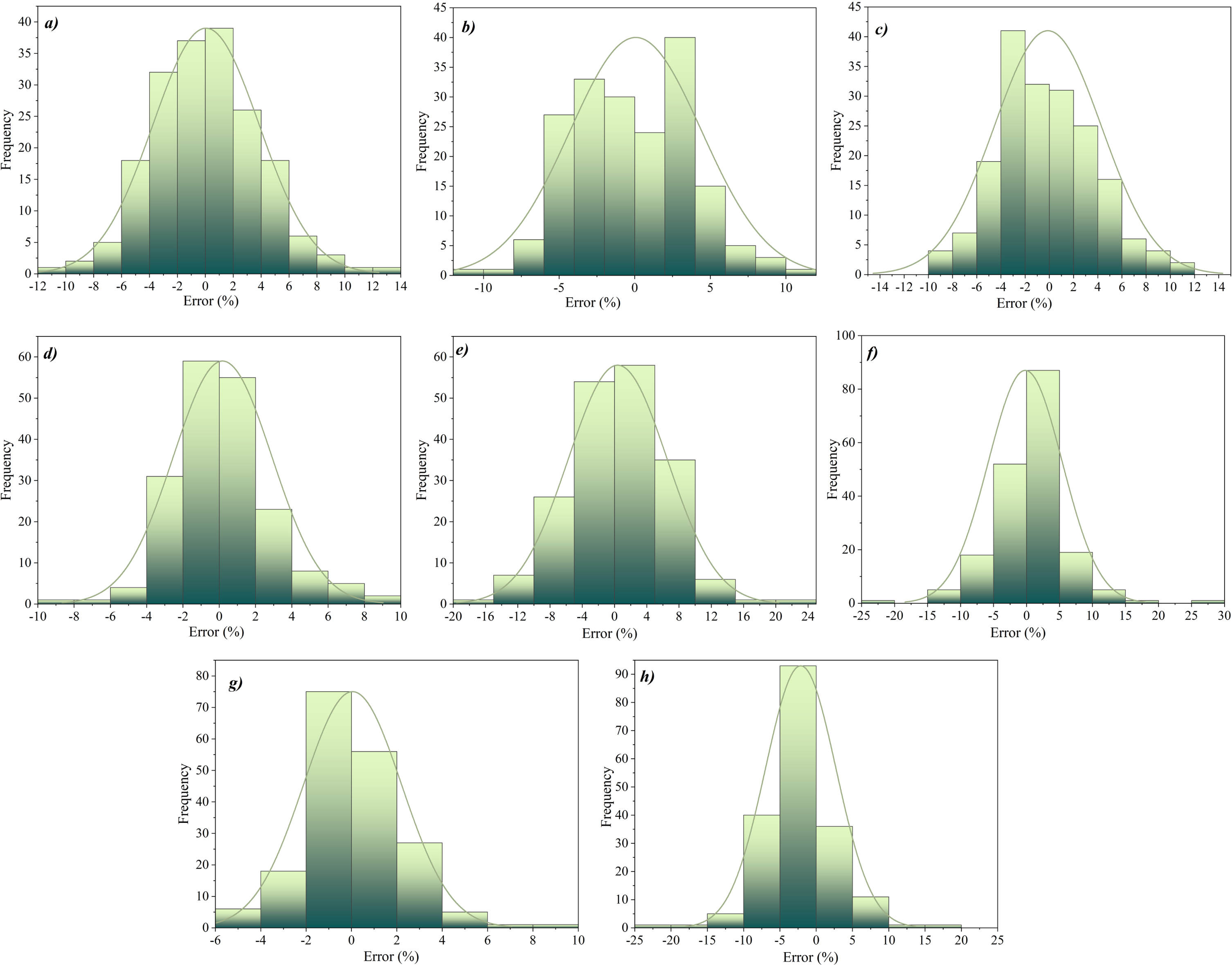
The histogram of developed models a) SVGO, b) DTGO, c) ADGO, d) SDA for compressive strength and e) SVGO, f) DTGO, g) ADGO, h) SDA for the Slump.

In the last section, Table 2 deals with the evaluation of k-fold-based hybrid models. Metrics include R², RMSE, MAE, and MAPE. In the Slump, ADGO achieved the highest R² value of 0.988, a 1% difference from the SVGO and DTGO models. In two metrics, RMSE and MAE, the lowest values belong to DTGO, equal to 3.90 and 1.60, respectively. Furthermore, the lowest MAPE belongs to SVGO with a value of 0.012. The results of the values show that the strongest and weakest performance in the murky cases is associated with DTGO and ADGO, alternatively. On the other hand, according to the given metrics, the CS models are compared. Acceptable operating models in R². But in general, the highest value of R² was obtained by ADGO. In the error-related indicators, i.e., RMSE, MAE, and MAPE, the lowest values of 1.119, 0.85, and 0.11, respectively, which is belong to ADGO.

Table 2

The metric evaluates based on k-fold

Model	Feature	SVGO	DTGO	ADGO
RMSE	Slump	4.0323	3.9059	3.9919
MAE		2.5475	1.6049	2.9199
MAPE		0.0124	0.745	1.4957
R²		0.9753	0.9768	0.988
RMSE	CS	3.2898	3.5307	1.119
MAE		2.5555	2.7998	0.8502
MAPE		0.0372	3.9858	0.0119
R²		0.9845	0.9822	0.9982

4 Conclusion

Concrete is a widely used material in the construction industry. Ordinary concrete cannot meet the needs of some structures, such as skyscrapers, tunnels, bridges, etc. For this reason, high-performance concrete (HPC) was developed that given compressive strength is boosted. Performing tests to find compressive strength and slump can be done in laboratory as costly hardware-based mode and efficient soft-based mode. In this regard, artificial intelligence is proposed to be able to estimate the compressive strength and Slump of HPC from machine learning methods. In this regard, predicting framework of Support Vector Regression (SVR), AdaBoost (ADA), Decision Trees (DT), was coupled with Chaos game optimization (CGO) algorithm as hybrid mode. Developing hybrid models was the main aim of the current paper that materials of HPC samples fed them to regenerate compressive strength and slump values. Beside hybrid models, ensemble model was created also to show the capability of hybrid models designed with new way of coupling.

The R² for hybrid ADGO model was the highest value (equal to 0.996), so its difference with DTGO and SVGO was 2%. Also, compared to the ensemble model, SDA has been able to perform better, with a difference of 1%. The next evaluation related to RMSE and the most acceptable performance is still ADGO which has a value equal to 1.609, which is a remarkable value compared to other models. ADGO has a difference of 61% with SVGO, and this difference with DTGO equals 64%. In addition, the RMSE of SDA is equal to 4.284, and its difference from ADGO is 62%. The SDA ensemble model for R² can achieve the highest value of 0.961, so the difference between DTGO and SVGO is 8 and 4 percent, respectively. Furthermore, ADGO’s RMSE equals 8.263, and its difference with SDA is 36%. In general, it can be stated that in the compressive strength of the ADGO composite model, it had a stronger performance, and DTGO had the weakest performance. On the other hand, SDA obtained the most suitable values for slump flow, and DTGO obtained the poorest values in a slump.

To sum up, hybrid models appeared more accurate than ensemble model, however, performance of ensemble framework was at the acceptable level. Even for modeling slump the correlation of modeled values with gauged ones, ensemble model was accurate. With considering such high correlation, possibility of using AI-based model instead of laboratory experiments is proved and economic and technical productivity would be brought up consequently.

References

Brandt

A.M.

, Fibre reinforced cement-based (FRC) composites after over 40 years of development in building and civil engineering, Compos. Struct. 86(1–3) (2008), 3–9.

Farnam

, Mohammadi

and Shekarchi

, Experimental and numerical investigations of low velocity impact behavior of high-performance fiber-reinforced cement based composite, Int. J. Impact Eng. 37(2) (2010), 220–229.

Breitenbuecher

High performance fiber concrete SIFCON for repairing environmental structures, in, Proceedings of the third RILEM/ACI workshop: high-performance fiber reinforced cement composites, London, UK (1999), 585–594.

Neville

A.M.

Properties of concrete 4. Longman London, 1995.

Aïtcin

P.-C.

High performance concrete. CRC Press, 1998.

Behnood

, Behnood

and Modiri

, Gharehveran and K.E. Alyamac, Prediction of the compressive strength of normal and high-performance concretes using M5P model tree algorithm, Constr. Build. Mater. 142 (2017), 199–207. doi: 10.1016/j.conbuildmat.2017.03.061.

Al-Shamiri

A.K.

, Kim

J.H.

, Yuan

T.-F.

and Yoon

Y.S.

, Modeling the compressive strength of high-strength concrete: An extreme learning approach, Constr. Build. Mater. 208 (2019), 204–219.

Chou

J.-S.

and Pham

A.-D.

, Enhanced artificial intelligence for ensemble approach to predicting high performance concrete compressive strength, Constr. Build. Mater. 49 (2013), 554–563. doi: 10.1016/j.conbuildmat.2013.08.078.

Benemaran

R.S.

and Esmaeili-Falak

, Optimization of cost and mechanical properties of concrete with admixtures using MARS and PSO, Comput. Concr. 26(4) (2020), 309–316.

10.

Huang

, Jiang

, Wang

, Zhu

and Afzal

, Prediction of long-term compressive strength of concrete with admixtures using hybrid swarm-based algorithms, Smart Struct. Syst. 29(3) (2022), 433–444.

11.

Gilan

S.S.

, Jovein

H.B.

and Ramezanianpour

A.A.

, Hybrid support vector regression–Particle swarm optimization for prediction of compressive strength and RCPT of concretes containing metakaolin, Constr. Build. Mater. 34 (2012), 321–329.

12.

Abd

A.M.

and Abd

S.M.

, Modelling the strength of lightweight foamed concrete using support vector machine (SVM), Case Stud. Constr. Mater. 6 (2017), 8–15. doi: 10.1016/j.cscm.2016.11.002.

13.

Kewalramani

M.A.

and Gupta

, Concrete compressive strength prediction using ultrasonic pulse velocity through artificial neural networks, Autom. Constr. 15(3) (2006), 374–379.

14.

Masoumi

, Najjar-Ghabel

, Safarzadeh

and Sadaghat

, Automatic calibration of the groundwater simulation model with high parameter dimensionality using sequential uncertainty fitting approach, Water Supply 20(8) (2020),3487–3501. doi: 10.2166/ws.2020.241.

15.

Kewalramani

M.A.

and Gupta

, Concrete compressive strength prediction using ultrasonic pulse velocity through artificial neural networks, Autom. Constr. 15(3) (2006), 374–379. doi: 10.1016/j.autcon.2005.07.003.

16.

Afzal

, Ziapour

B.M.

, Shokri

, Shakibi

and Sobhani

, Building energy consumption prediction using multilayer perceptron neural network-assisted models; comparison of different optimization algorithms, Energy (2023), 128446. doi: 10.1016/j.energy.2023.128446.

17.

Schapire

R.E.

Explaining adaboost, in, Empirical inference, Springer, (2013), 37–52.

18.

Erdal

H.I.

, Two-level and hybrid ensembles of decision trees for high performance concrete compressive strength prediction, Eng. Appl. Artif. Intell. 26(7) (2013), 1689–1697.

19.

Cağlar

Predicting the compressive strength and slump of high strength concrete using neural network, 2006.

20.

Yeh

I.-C.

, Exploring concrete slump model using artificial neural networks, J. Comput. Civ. Eng. 20(3) (2006), 217–221.

21.

, Li

and Nguyen

T.N.

, A novel optimised self-learning method for compressive strength prediction of high performance concrete, Constr. Build. Mater. 184 (2018), 229–247.

22.

Mousavi

S.M.

, Aminian

, Gandomi

A.H.

, Alavi

A.H.

and Bolandi

, A new predictive model for compressive strength of HPC using gene expression programming, Adv. Eng. Softw. 45(1) (2012), 105–114. doi: 10.1016/j.advengsoft.2011.09.014.

23.

Freund

and Schapire

R.E.

, A decision-theoretic generalization of on-line learning and an application to boosting, J. Comput. Syst. Sci. 55(1) (1997), 119–139.

24.

Stein

, Chen

, Wu

A.S.

and Hua

K.A.

, Decision tree classifier for network intrusion detection with GA-based feature selection, in Proceedings of the 43rd annual Southeast regional conference-Volume 2 (2005), 136–141.

25.

Damanik

I.S.

, Windarto

A.P.

, Wanto

, Andani

S.R.

and Saputra

, Decision tree optimization in C4. 5 algorithm using genetic algorithm, in, Journal of Physics: Conference Series 1255(1) (2019), 12012.

26.

Barros

R.C.

, Basgalupp

M.P.

and De

A.C.

, Carvalho and A.A. Freitas, A survey of evolutionary algorithms for decision-tree induction, IEEE Trans. Syst. Man, Cybern. Part C (Applications Rev. 42(3) (2011), 291–312.

27.

Gupta

A self explanatory review of decision tree classifiers, in International conference on recent advances and innovations in engineering (ICRAIE-2014) (2014), 1–7.

28.

P.-S.

, Chen

S.-T.

and Chang

I.-F.

, Support vector regression for real-time flood stage forecasting, J. Hydrol. 328(3–4) (2006), 704–716.

29.

Zhang

, Sato

and Iai

, Support vector regression for on-line health monitoring of large-scale structures, Struct. Saf. 28(4) (2006), 392–406.

30.

, Huang

, Gao

and Zhao

, Fast and robust text detection in images and video frames, Image Vis. Comput. 23(6) (2005), 565–576.

31.

Talatahari

and Azizi

, Optimization of constrained mathematical and engineering design problems using chaos game optimization,Comput. {&}, Ind. Eng. 145 2020 p.106560.

32.

Lim

C.-H.

, Yoon

Y.-S.

and Kim

J.-H.

, Genetic algorithm in mix proportioning of high-performance concrete, , Cem. Concr. Res. 34(3) (2004), 409–420. doi: 10.1016/j.cemconres.2003.08.018.

33.

Bartlett

, Freund

, Lee

W.S.

and Schapire

R.E.

, Boosting the margin:Anewexplanation for the effectiveness of voting methods, Ann. Stat. 26(5) (1998), 1651–1686.

34.

Vapnik

V.N.

Controlling the generalization ability of learning processes, in The Nature of Statistical Learning Theory, Springer (2000), 93–122.

35.

, Li

, Yang

and Wen

, Wavelet support vector machine-based prediction model of dam deformation, Mech. Syst. Signal Process. 110 (2018), 412–427.

36.

Smola

A.J.

and Schölkopf

, A tutorial on support vector regression, Stat. Comput. 14(3) (2004), 199–222. 10.1023/B:STCO.0000035301.49549.88.

Applying machine learning techniques in the form of ensemble and hybrid models to appraise hardness properties of high-performance concrete

Abstract

Keywords

1 Introduction

2.1 Data gathering

References