Deep convolutional neural network for glaucoma detection based on image classification

Abstract

PURPOSE:

Many researchers have found that the improvement in computerised medical imaging has pushed them to their limits in terms of developing automated algorithms for the identification of illness without the need for human participation. The diagnosis of glaucoma, among other eye illnesses, has continued to be one of the most difficult tasks in the area of medicine. Because there are not enough skilled specialists and there are a lot of patients seeking treatment from ophthalmologists, we have been encouraged to build efficient computer-based diagnostic methods that can assist medical professionals in early diagnosis and help reduce the amount of time and effort they spend working on healthy situations. The Optic Disc position is determined with the help of the LoG operator, and a Disc Image map is projected with the help of a U-net architecture by utilising the location and intensity profile of the optic disc. After this, a Generative adversarial network is suggested as a possible solution for segmenting the disc border. In order to verify the performance of the model, a well-defined investigation is carried out on many retinal datasets. The usage of a multi-encoder U-net framework for optic cup segmentation is the second key addition made by this proposed work. This framework greatly outperforms the state-of-the-art in this area. The suggested algorithms have been tested on public standard datasets such as Drishti-GS, Origa, and Refugee, as well as a private community camp-based difficult dataset obtained from the All-India Institute of Medical Sciences (AIIMS), Delhi. All of these datasets have been verified. In conclusion, we have shown some positive outcomes for the detection of diseases. The unique strategy for glaucoma treatment is called ensemble learning, and it combines clinically meaningful characteristics with a deep Convolutional Neural Network.

1 Introduction

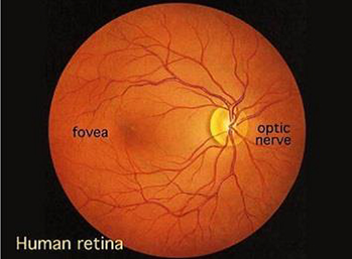
Research and clinical applications make extensive use of retinal images all around the world. This makes retinal images a primary class in the medical domain datasets. For instance, in the evolution of illness, researching early diagnosis, developing risk profiles, and classifying disease kinds, among other things, are all important. A fundus or retinal image is basically a depiction of the internal surface of the eye and comprises a variety of distinct anatomical components (features), such as the optic disc, macula, fovea, and blood vessels, amongst other things [1]. Through the use of retinal pictures, the evaluation of the retina has become more accurate, dependable, and quantitative. In clinical situations, medical professionals search for main symptoms to identify any abnormality that may be present in a picture of the fundus. The quantitative information supplied by retinal pictures helps in better understanding between healthy and diseased images, whilst the qualitative information offered by retinal images assists in determining the severity of the illness. When making a diagnosis of a condition affecting the retina, ophthalmologists practised in a clinical situation look for certain signals in the retina [2]. During a diagnostic examination of the fundus using ophthalmoscopy and/or fundus photography, the pupil of the eye is first dilated with eye drops in order to allow for a much larger area of observation of the back of the eye. Next, a specialised device known as a fundus camera is used to focus the light on the fundus. Finally, a diagnosis is made based on the findings of the examination. In the course of the previous several decades, both the technology and the models used in fundus photography have seen significant development and evolution [3].

It is possible to characterise the optical design of the fundus camera by referring to an indirect ophthalmoscope. When the light enters the eye via the pupil and strikes the retina, it creates a picture that is an inverted and enlarged representation of the fundus. Because an automated analysis is conducted using digital pictures, image quality is of utmost importance, and the pixel resolution is what determines image quality. In the event that the resolution is low, it is possible that some of the small-scale indications, such as microaneurysms, will not be apparent. On the other hand, high-resolution photographs need a greater amount of work to process. The normal camera has a magnification scale of 2.5x and may show an area of the retina of 30 by 50 pixels [4]. Additionally, certain upgraded versions of the camera can give a magnification of 5x. Recently, there has been a rise in interest in portable low-cost retinal cameras, particularly for use in the context of community camps and healthcare facilities. Depending on the application or usage, some of these devices provide great image quality while putting a focus on simple mobility, while others give a very low-cost device with mediocre imaging quality, and a few of them are based on easy assembly, which involves adding an adapter to cellphones. In general, they have drawbacks in terms of acceptable picture quality, such as poor contrast and significant reflection artefacts, particularly when the field of view (FOV) is modest to large. Ophthalmologists examine, diagnose, and treat eye illnesses with the use of retinal pictures [5]. Some of these diseases include glaucoma, age-related macular degeneration (AMD), and diabetic retinopathy (DR), amongst others. In general, a fundus photograph is a two-dimensional view of the retina, and it is commonly used for analysis. However, with the advancement of technology, there exists another imaging technique known as optical coherence tomography (OCT), which gives a cross-sectional view of the retina for the identification and assessment of any abnormalities, and is, as a result, an extremely powerful tool [6]. Constructive interference is the basis of this non-invasive, high-resolution optical imaging system that relies on light reflected off the object being studied as its source of illumination. It enables improved depth resolution and creates real-time pictures of cross-sections of ocular tissues. In addition, spectral domain optical coherence tomography, often known as Fourier OCT or SD-OCT, is the most recent technical variation of this developing modality. Nevertheless, the cost of these technologies is quite high, and there are problems with their portability.

As was noted before, the incidence of eye illnesses is increasing at a frighteningly rapid pace, with glaucoma being the second major cause of blindness throughout the globe and the third leading cause in India. According to the findings of several scientific studies, irreversible eyesight loss may be avoided in at least sixty percent of instances if an accurate early diagnosis and therapy are administered during the first stages of the condition. As a consequence of this, there is a critical need for accurate computer-aided interpretation of digitised fundus pictures. In spite of the vast quantities of work that are now accessible in the area of medical research for the purpose of glaucoma diagnosis, all of those algorithms are only applicable in a laboratory setting [7]. In spite of all the research that has been done up to this point, there is no such strategy that is trustworthy for a significant number of datasets and generalises very well. All of the previously developed techniques provide a performance that is acceptable for a specific number of datasets, but it is possible that they deliver a performance that is not satisfactory for other datasets. The majority of techniques for pathological pictures, often known as images that depict illnesses. For instance, segmenting the optic disc is a simple operation when the retina is in good condition, but it may become a time-consuming chore when atrophies and abnormalities are present. It is vital to design methods that are computationally efficient and can handle a multi-variety of pathological states in a glaucoma picture as a result of the introduction of automated glaucoma [8] detection tools and the consequent improvement in machine learning algorithms. This is because it is becoming more important to implement such approaches. This study was driven to design an automated method by the need for population-based early diagnosis of retinal illnesses using fundus imaging. Fundus imaging may be used to examine the retina. In the field of research, the following are some of the most important considerations that led to the execution of the task that was proposed:

The vast majority of automated glaucoma detection algorithms have problems with generalisation. This means that an algorithm that was developed for a specific job may only perform exceptionally well for a specific dataset. Therefore, the use of any approach, regardless matter how great its sensitivity, is constrained by the need for only modest specificity. This dilemma has to be solved using well-trained deep learning models that take into account the disease’s most reliable early warning signs.

There is an undeniable need in the medical industry for the use of automated diagnostics for two primary reasons. According to data provided by the Glaucoma Society of India, the incidence of the condition has increased by a factor of four since the year 1980 [9]. The most significant obstacle is presented by underdeveloped nations such as India, where the number of patients treated by a single ophthalmologist is around 105 to 1. In addition to this, there is an insufficient amount of competent labour available, which is another significant risk. For this reason, governments are employing optometrists, nurses, or skilled image graders to do screening utilising retinal scans. Glaucoma screenings are performed with the intention of identifying any early warning symptoms that may be present in the eye prior to the onset of irreversible vision loss [10]. The second test for the condition is regarded to be the pinnacle of the preventative measures that may be taken to guard against irreversible eyesight loss. 3. Tele-ophthalmology has a significant potential to reach geographical regions with limited access to medical resources and to deliver high-quality medical care in such locations. Ophthalmologists will require assistance in disease diagnosis procedures [11], thus it is necessary to design an automated diagnostic system that is both cost-effective and efficient. This will allow medical professionals to better manage situations like the one described above. These kinds of technologies not only help physicians, but they also cut down on the amount of work that has to be done to analyse a healthy population. As a consequence of this, the only people who need to be sent to an ophthalmologist are those individuals [12] who the system has reason to believe are sick. The primary focus of this proposed work work is the creation of automated, reliable, and effective segmentation and detection systems.

The qualitative evaluation of the eye may be made more repeatable and objective with the use of computer approaches, which are utilised in retinal image analysis. For the sake of diagnosis and establishing a baseline, ophthalmologists are required to provide a qualitative and quantitative description of their ophthalmoscopy impression of the optic nerves. This allows for the change in condition to be identified via inspection. Glaucoma, a condition that may cause permanent vision loss, is being investigated in this study so that researchers can monitor its development and alert patients to any changes that may help them preserve their eyesight. The following is a list of issues that have been discovered with some of the present procedures for assessing glaucoma: The Cup to Disc Ratio (CDR) in glaucoma diagnosis is determined by a quantitative impression of the optic nerve. The CDR has significant issues that limit its computation accuracy (an inconsistency is reported in while explaining the quantitative damage of the OD caused by glaucoma). This is despite the fact that it has advantages such as being easy to use and having fewer artefacts caused by magnification of less than 25 times, all of which may be very appealing. When determining CDR, disc diameter is not taken into consideration; as a result, both false positive and false negative perceptions are possible. CDR focuses on the optic cup, while the true anatomical change that occurs in glaucoma is the breakdown of tissues around the neuro-retinal rim. For instance, some participants have a low CDR but exhibit a major reduction in their visual field, whilst other subjects show a higher CDR but just a moderate reduction in their visual field. This is mostly due to the problems with CDR, which cannot account for the various configurations of the optic cup, including the neural retinal rim and focused notching, both of which pertain to the local cup expansion area. The CDR staging method does not take disc size into consideration, and the focal narrowing of the neuro-retinal rim is not emphasised in an appropriate manner. Because of all of these problems, using the CDR to make accurate diagnoses is not as effective as it might be. If CDR alone is employed as a criteria for damage, then there is a possibility that big optic nerves may be wrongly labelled as glaucomatous and little optic nerves will be considered normal. This is because large optic nerves have a higher CDR than small optic nerves do. Along with other common risk variables including race, age, gender, family history, demographic conditions, and retinal abnormalities, the system may be combined with current ophthalmologic trials and clinical evaluations if a predetermined clinical method is followed. The fundus image analysis that was suggested in the study was an effort to overcome the subjective or operative variability, analyse the picture automatically without requiring any interaction from a human, and do so without the need for any human intervention. The primary goal is to build a feature extraction and segmentation strategy for diagnosing abnormality and normalcy of glaucoma illness utilising public databases such as HRF, RIMONE, STARE, and DRIVE as well as local datasets. This will be accomplished via the use of local datasets. In addition, the goals for glaucoma illness identification utilising machine learning approaches are going to be presented in the chapters that are coming up after this one.

The organization of paper is as follows; section 2 includes background study of exiting work; section 3 includes proposed methodology; section 4 includes experimental analysis of proposed work; section 5 includes conclusion and future work.

2 Background study

The optic disc is not only the part of the retina that contains the brightest circular landmark, but it is also the region where the blood veins of the retina converge. Numerous studies have made advantage of this characteristic in conjunction with high-intensity natural settings. However, in order to use this procedure, the retinal blood vessels must first be segmented. This is a necessary prerequisite. In order to find the OD This fuzzy convergence characteristic of blood vessels is used as the principal feature of [13], together with the maximum brightness property of the optic disc in the equalised picture of the retina. [14] employs these two properties in combination with one another. [15] takes a technique that is quite similar to this one and models the geometrical organisation of major blood vessels in order to identify OD. It is organised according to the parabolic pattern of two main retinal blood veins that lie in the nasal and temporal regions and share a common vertex. The mathematical models are predicated on the symmetric assumption of the vascular structure, and they determine the two primary model parameters, which are the aperture (a) and vertex (xOD, yOD) of a parabola, based on the data from the training set, which is comprised of vessel points. Using retinal pictures, [16] suggests developing a method that is based on the vascular distribution and directional properties of the retina. After applying the Gabor filter to the green channel picture, the binary vessel structure can be recovered. There are twelve distinct orientations of a filter that are selected, and the direction of the filter that produces the greatest magnitude is the one that is taken into consideration for the final response of the Gabor filter. To accomplish this, a vessel distribution feature is used. This feature incorporates vessel compactness, vessel homogeneity, and vessel density as its primary characteristics. In order to determine the column ordinate of OD, this feature set is applied all the way across the horizontal axis of the picture. In conclusion, the strategy of fitting a parabola along the selected vertical axis is shown. This approach is based on the generic Hough transform. The row ordinate that corresponds to the OD center’s position 33 serves as an identifier for the parabola’s vertex. This approach enables accurate and speedy identification across a wide variety of datasets. [17] proposes yet another method of OD detection that takes place inside the vessel. The first step is to do thresholding on the red channel so that ROI may be extracted. In order to get a higher contrast in the final picture, the adaptive histogram equalisation technique is used. The technique for extracting blood vessels is carried out, and a straightforward approach to edge fitting is used, as recommended in [18]. The orientation of the direction-matched filter is correlated with the orientation of the vessels that are present at the OD in order to establish the location of the OD. For the purpose of performing a unique method for quickly localising the optic disc, [19] suggests doing a local fractal analysis on a blood vessel map. Only the areas surrounding the prospective hotspots with the highest intensity are investigated in order to keep the computational complexity low. The approach is based on the idea that the region where blood vessels merge together has the maximum fractal Df dimension in comparison to other big bright areas in retinal pictures, such as hard exudates and artefacts (which have few blood vessels inside and surrounding them). This allows the system to function correctly. Based on vector field theory and its application to directed blood arteries, [20] have developed yet another approach for the identification of discs. An important step forward in this field was taken by the author of [21], who provided a solution to the issue by assuming the position of the optic disc and the fovea in relation to one another in order to find a solution. The location of these anatomical landmarks may be predicted with the use of a KNN regressor by employing a collection of data derived from the vascular map. These features include the number of vessels, the breadth of blood vessels, the standard deviation of vessel width and orientation, and so on. An strategy that is based on a histogram and is proposed by [22], in which the top 0.5% grey level intensities in the red channel are selected as candidate locations. The picture is then further split into sixty-four smaller sections, and the portion of the image that corresponds to the highest possible number of candidate pixels is chosen to constitute the optic disc. An additional pre-processing step is carried out by it in order to lessen or get rid of the dazzling fringes that are present at the field-of-view (FOV) perimeter. A sparse space-based sub-image classification has been developed for the purpose of localising the optic disc in the work that is described in [23]. It presents the issue of OD detection as a classification problem, in which a test sub-image is categorised as either containing OD or not containing OD. To represent each sub-image as a sparse linear combination of the dictionary atoms, a dictionary of OD samples is generated first. Each sub-image is then expressed. The chosen sub-image is convolved with a Laplacian of Gaussian (LOG) blob detector so that the OD centre coordinate may be located. In order to find the OD using the conventional picture matching methods, recommended using a template matching and vessel convergence characteristics. In this method, OD candidates are chosen based on template matching performed with an adaptable template size in CIELab’s lightness picture. In addition, the vessel merging feature is employed in order to obtain the position on the OD surface and steer clear of false-positive zones. In a unique approach that is based on image processing methods is offered. In this methodology, an initial picture has a series of iterative opening-closing morphological operations carried out on it in order to produce an improved brilliant image. The process of iterative morphology is carried out in order to gradually get rid of the little brilliant structure (also known as hard exudates) that is present in the retinal picture. In a manner similar to the vessel geometric model presented investigates the retinal vascular geometry for the OD position. It focuses less on two big parabolas that are attached to the primary vessel and more on a local directional model that is included into the design. Constructing the local model involves determining the local vessel convergence at OD, in addition to the form and brightness of OD. At long last, a hybrid directional model built from both global and local models is presented for consideration. Using concepts from image processing, [18] suggests another template matching approach that may be implemented in the coloured plane histogram. As a result of the varying OD sizes present in retinal pictures, several templates are used in accordance with the requirements of the database.

Fig. 1

A Sample Glaucoma Fundus Image Obtained from Fundus Camera.

We have found that the majority of the algorithms for detecting optic discs that have been presented in the published research are based on the intensity variation and circular characteristic of optic discs. This leads in poor results for low resolution, fuzzy, and artefact pictures. The first contribution suggests a U-Net design for the creation of Distance Intensity maps utilising Tuckey’s biweight loss function, which can withstand the presence of outliers. This will allow the restriction to be circumvented. In addition, as of yet, there has been no research conducted to investigate the inter-dataset performance of the optic disc segmentation approach. The disc extraction process is carried out with the assistance of a generative adversarial network. The following contribution was inspired by the capability of U-net designs for the segmentation of biological images. Instead of the traditional design of a U-net, we provide a multi-encoder U-net (or Y-net) framework for superior feature enrichment in the optic cup segmentation technique. ˆ Using the most recent developments in image processing and deep learning methods, researchers have been attempting to identify peripapillary atrophy for a significant amount of time. This is something that we have seen. The majority of these cutting-edge algorithms either employ raw picture information for categorization or depend on some kind of feature extraction process to understand the data. This may prove to be a difficult undertaking because of the difficulty in choosing the appropriate or best collection of characteristics that may bring about an improvement in the accuracy. The third component diagnoses PPA by using deep convolutional neural networks in conjunction with statistical characteristics that have been carefully constructed by hand. In addition to this, the difficult task of RNFL loss detection is accomplished with the help of an active transfer learning framework applied to a restricted private dataset. The performance of the suggested approach is superior than that of the most recent algorithms. The need to diagnose glaucoma using an ensemble of multi-prediction models for glaucoma provided the impetus for the last contribution to the proposed work. In the research that has been done on how to diagnose it, CDR-based aspects have been investigated; nevertheless, we suggest an ensemble of multi clinical indications of glaucoma.

According to our understanding, the diagnosis of retinal nerve fibre layer (RNFL) defects using digital fundus images has been proposed by a few studies. The majority of approaches focus on doing a local texture analysis of the RNFL loss area by making use of a variety of statistical and directional variables. In order to improve the appearance of almost vertical black bands in the polar converted fundus picture, the author suggests using a Gabor filter in the processing. The portion of the RNFL that has been lost, which corresponds to pixels with mean values that are lower than a threshold. One such piece of research that uses a polar converted retinal picture, which uses a Gabor filter to increase vertical band contrast. The employment of filters with varying sizes and properties, followed by the use of an artificial neural network (ANN) classifier with three layers, is the main contribution of this study. 48 Gaussian Markov random fields (GMRF) are used for RNFL layer texture analysis in the research presented. The Bayesian classifier is used to categorise the tiny square-shaped patches that measure pixels on each side. at another addition two distinct algorithms are used at the outer border of the fundus and close to the optic disc (referred to as the OD, henceforth) in order to determine the severity of the RNFL defect. It differentiates between normal and defective regions by using the intensity feature of the image. The non-blood vessel portion of the retina was used for feature (spectral, brightness, and edge-based) computation in the study’s deep retinal vascular precise segmentation technique for RNFL identification. A neural network with one hidden layer and two neurons is used to classify the blocks from the region of interest (the area surrounding the optic disc) as either having a healthy retinal nerve fibre layer or an area that has degraded. In the paper a strategy that is based on the dissimilarity of features between the candidate and its associated background is suggested, in addition to an anisotropic diffusion-based smoothing technique.

[23] uses both colour and texture features to create the difference feature vector between the candidate area and the surrounding region. This is done so that it may integrate the global characteristics. For the final RNFL prediction, a mixture of judgements acquired from several classifiers, such as k-NN, Nearest Mean Scaled and Linear discriminant, etc., is employed. Another polar transform-based method for RNFL defect identification is suggested in the work of which makes use of the Hough transformation to pick candidate areas that include straight lines. The technique classifies the ROI (region outside the OD) using an ensemble RUSBoosted tree classifier using the coarseness texture feature. Recent research published in [9] proposes a deep learning-based method that uses seven CNN layers for patch-based RNFL defect classification on green channel training patches.

3 Proposed method

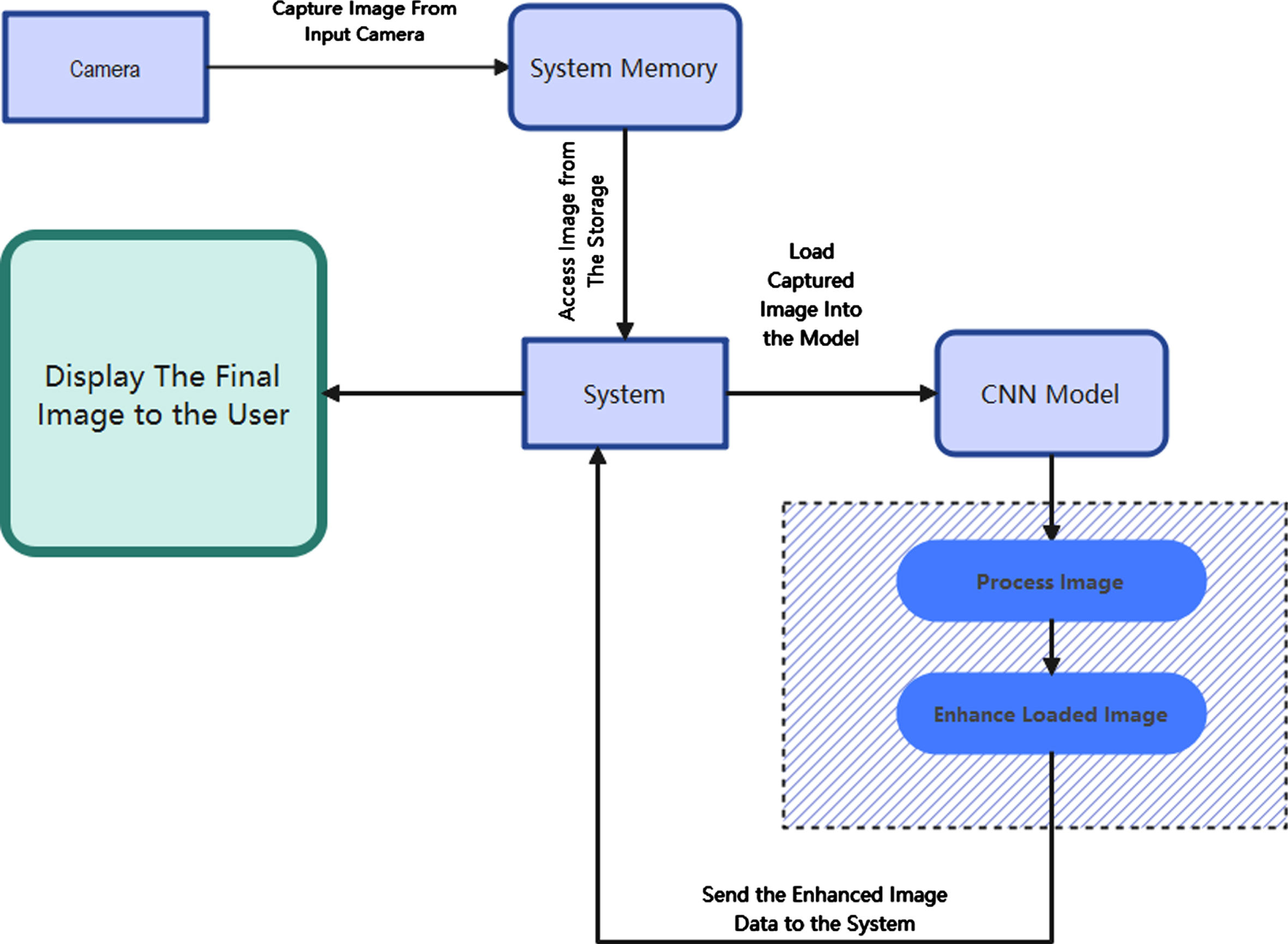
The identification of glaucoma relies heavily on the use of automated techniques for pre-processing and segmentation of images. It is common for the presence of blood vessels to impede the process of segmenting Optic Disc (OD) and Optic Cup (OC). An algorithm for the automatic identification and exclusion of blood vessels is thus suggested as a stage in the processing that comes before it. The OD and OC are segmented using the pre-processed fundus Images as the source material. It is suggested to use an automated approach for the segmentation of OD from the already preprocessed fundus pictures. The OD segmentation technique that has been presented makes use of statistical characteristics, an approach known as circle finding, and a decision tree classifier. The suggested approach for OC segmentation attempts to improve the OC region by developing a new channel in order to compensate for the decreased degree of variability that exists between the pixels of OD and OC. Because the threshold value determined for the segmentation techniques is consistent across all datasets, it has the potential to be useful for a wide variety of glaucoma datasets. The following list summarises the most important contributions made by this chapter:

Pre-Processing Carried out using Gaussian Filter and morphological Algorithm.

New methods for reliable OD and OC segmentation are created, which overcome the decreased variability that is present between the pixels of OD and OC. Figure 2 provides a visual representation of the whole system.

Fig. 2

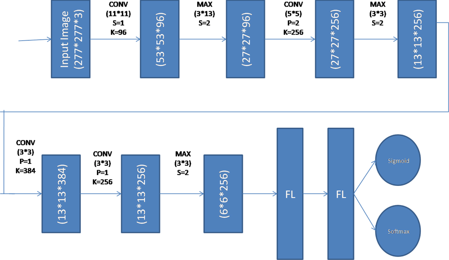
The architecture of the Deep Convolutional Neural Network.

3.1 Image dataset

These fundus Images were obtained at Kasturba Medical College (KMC), located in Manipal, India. KMC has contributed a total of 300 photographs, 95 of which are considered normal and 205 of which are considered to have glaucoma. The Zeiss FF450 plus fundus camera was used to take these photographs. The Images are taken from the perspective of the posterior pole, which encompasses both the optic disc and the macula. The pixel dimensions of the picture are 2588 by 1958. Annotations have been supplied by the ophthalmologist for each of the 300 Images in the collection. Additionally, the KMC’s ethical committee has given its blessing for the collecting of data to be used in research. 2. The Drishti dataset is presently one that is accessible to the public. The picture collection is being made publicly available to encourage research into glaucoma detection. The collection includes 101 Images total, including 31 healthy and 70 glaucomatous specimens. The Aravind Eye Hospital in Madurai, India, provides the annotations for the Images, which were shot at a resolution of 2896 by 1944 pixels. The ophthalmologist has kindly supplied us with the comments for these Images.

3.2 Image pre-processing

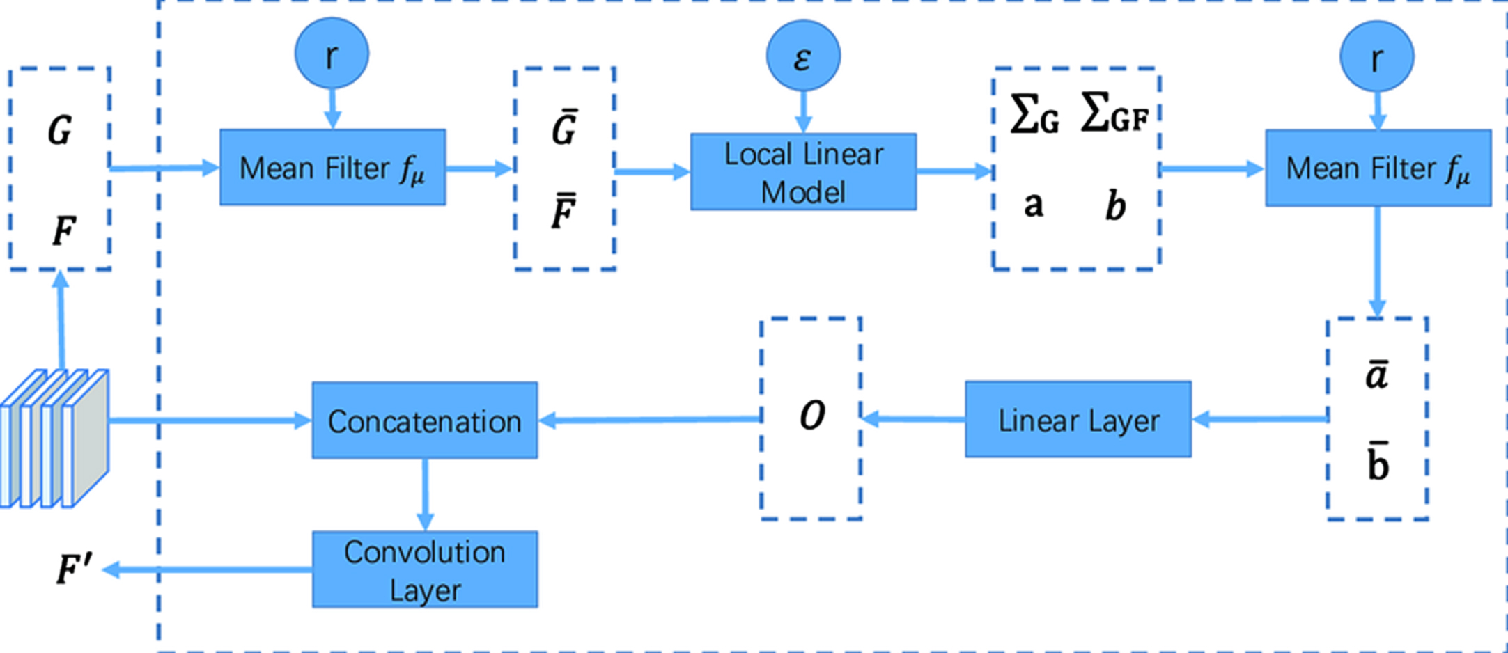
During the process of distinguishing between OD and OC, the presence of blood vessels in the fundus pictures might lead to uncertainty. Therefore, as a first stage in the procedure. It has been determined that there are no blood vessels present and they have been excluded. The green channel of the RGB picture must be selected as the starting point for the procedure used to extract the blood vessels from the image. In comparison to the red and blue channels, the blood vessels are substantially more visible in the green channel of the RGB picture. In order to get rid of noise in the image’s green channel, a 2D Gaussian smoothing kernel has been used. This kernel has a standard deviation value that is provided by the symbol. This results in a Gaussian filtered picture, denoted by the notation F(x,y). In addition to this, a linear structuring element that has orientations that range from 0 to 360 degrees in increments of 45 degrees is applied. Because the contrast of the blood vessels is so low in comparison to the image’s backdrop, this is the option that should be chosen. After the morphological dilation and erosion operation has been carried out, the response image, which is denoted by F_1 (x,y), is subtracted from the picture that has been filtered using a Gaussian. The answers are totaled together in order to highlight the blood vessels that are irregularly dispersed across the picture (F_“total” (x,y)). The value of the scaling constant is changed throughout a collection of 20 Images in order to generate the Gaussian filtered image. This is done by cycling through all of the available possibilities. The identification of blood vessels is improved by using the number = 4, which stands for four. The Images that were acquired had a smooth appearance when the value was less than four, but when the value was more than four, the images were unsuitable for processing owing to a loss of image information. After that, the vessel augmented picture is thresholded by choosing a threshold value that was acquired by the Otsu thresholding technique. The Otsu thresholding approaches are used because of their malleability, straightforwardness, and resiliency. The Otsu threshold approach determines an ideal threshold value by maximising the between-class variation of the grey levels that are present in the object and background area. This is accomplished by selecting a threshold value that is optimum. After that, the morphological dilation operation is performed on the picture of the vessel that was removed. The process of making things in a picture seem more substantial is referred to as dilation. Length 9 and angle (in degrees) 0 are the ideal dimensions for a linear structuring element to utilise when performing a dilation operation.

Local Mean of Pixel(μ) $\mu =1\mathit{NMI}\left(x,y\right)$(1)

Local Variance(σ) $\left({\sigma }^2\right)=1{\mathit{NMI}}_2\left(x,y\right)-{\mu }^2$(2)

R channels are quite big, and there is a lack of contrast between the blood vessels and the rest of the picture. The brightness and contrast of the B channels are the lowest when compared to those of the other three channels. After the noise has been removed, the next step in the image convolution process involves altering the pixel value at each input picture coordinate by applying a mean weighted kernel to the pixels that are adjacent to that location. The procedure is repeated in order to produce a fresh matrix of the picture that is being taken into consideration.

Every individual pixel is available with a set of surrounding neighbourhood pixels, with a predefined set of mass that every individual pixel is available with a set of surrounding neighbourhood pixels, with a predefined set of mass that is a weighted kernel and is considered for computing the filtered output value. Every individual pixel is available with a set of surrounding neighbourhood pixels, with a predefined set of mass that is a weighted kernel. The value calculated for a pixel located in the image (I) using a kernel K with a size of XX Y may be expressed as follows: $\begin{array}{cc}\hfill & I_{\mathit{new}}\left(i,j\right)=\sum s=-\mathit{AA}\sum t\hfill \\ \hfill & =-\mathit{BBK}\left(s,t\right)I\left(i+s,j+t\right)\hfill \end{array}$(3)

With the premise of lossless generality that the domain under consideration is a two-dimensional picture, the output Inew denotes the new output image. If X and Y are both odd integers and the kernel K is a collection of values that are symmetric along the x and y axes, then A = (X 1)/2 and B = (Y 1)/2 respectively.

A kernel with dimensions three by three is used as an illustration in Fig. 3, which depicts the process of the proposed filter. The independent calculation that is performed using a frame that has been specified enables this filter to function quickly and effectively. Only pixels that are close by are employed in the computation, which is critical for maintaining a high level of spatial consistency when access to memory (see Fig. 3).

Fig. 3

Computation of Proposed Filter.

3.3 Semi-supervised GAN for fundus image classification

The generator (G) model creates sample data by taking a random noise as input z from some random distribution p(z). The job of the discriminator (D) model is to identify whether the sample is from a genuine data instance p(x) or a produced sample p(z). In Equation 4, both the generator and the discriminator are trained to optimise the single objective function; however, the discriminator’s aim is to reduce the objective function, while the generator’s goal is to increase it. $\begin{array}{cc}\hfill & minmaxV\left(G,D\right)=E_{x\sim p\left(x\right)}\left[\mathit{log}D\left(x\right)\right]\hfill \\ \hfill & +E_{z\sim p\left(z\right)}\left[\mathit{log}\left(1-D\left(G\left(Z\right)\right)\right)\right]\hfill \end{array}$(4)

Deep Convolutional Neural Network was used in the process of creating the Discriminator model. This model has a total of 5 layers: 3 convolutional layers, 3 Max Pooling layers, 2 flatten layers, and 2 output layers. For supervised learning (as a multiclass classification), the output layer is built using a Softmax activation function, while for unsupervised learning (as a binary classification), sigmoid activation functions are used. Figure 3 presents the complete structured model for your perusal.

The total training procedure is broken up into two distinct phases: in Phase 1, the discriminator is fed true instances from the labelled dataset as well as fake samples generated by the generator. In Phase 2, the discriminator is fed false samples generated by the generator. The samples are analysed by the discriminator, and based on its findings, it determines whether the samples came from a genuine data distribution or from a generator. The true data instances are tagged as “(x1, y1), (x2, y2), (x3, y3)..... (xn,yk),” but the generator samples are labelled as a fake class. Algorithm of proposed work is shown below;

Algorithm 1. Pseudo code of proposed work
1. Initialise a image π θ  (a ∣ s) which is parametrised by θ and maps states s to actions a.
2. Sample {s i , a i } from image π θ  (a ∣ s)and run them.
3. Update the parameters φ of the Deep Neural Network (DNN), which approximates the value function ${\hat{V}}_{\phi }^{\pi }\left(s\right)$ based on sampled states, actions, and received rewards, r (s i , a i ).
4. Evaluate ${\hat{A}}^{\pi }\left(s_i,a_i\right)=r\left(s_i,a_i\right)+{\hat{V}}_{\phi }^{\pi }\left(s_i\left(t+1\right)\right)-{\hat{V}}_{\phi }^{\pi }\left(s_i\left(t\right)\right)$
5. Estimate the cost gradient ${\nabla }_{\theta }J\left(\theta \right)\approx {\sum }_i{\nabla }_{\theta }\log \left({\pi }_{\theta }\left(a_i\mid s_i\right)\right){\hat{A}}^{\pi }\left(s_i,a_i\right)$

Fig. 4

Discriminator Model in Semi-Supervised GAN.

Table 1

Comparison of PSNR Values

Image	Mean Filter	Median Filter	Weiner Filter	Adaptive Filter	Proposed Filter
Image1.jpg	83.62	74.22	54.71	60.52	91.27
Image2.jpg	82.17	73.62	56.76	62.43	90.82
Image3.jpg	84.21	73.52	57.44	62.42	90.27
Image4.jpg	85.33	73.18	57.38	61.32	91.69
Image5.jpg	84.18	74.32	55.04	61.53	91.50

Conventional techniques of supervised learning are used throughout the learning process of the discriminator, which involves the categorization of inputs into several groups. In order to do multi-class classification, the output function of the discriminator has to be altered. Both the generating function G(z) and the discriminator function D(x) are subject to an update in order to reach the minimum-maximum value of the same goal function or loss function. Let us assume that D(x) is a differentiable neural network function that, for samples taken from a genuine labelled dataset, generates the probability Pmodel (y = 1, 2...k |x), and that, for samples taken from an unlabeled dataset, generates the probability Pmodel (y = false|x). During Phase-II, the discriminator is fed genuine examples from the unlabeled dataset as well as false samples generated by the generator function G(z) in order to learn important features from the unlabeled dataset. The discriminator neural network’s output function is the sigmoid function, which classifies whether the provided sample is from the true data distribution or samples that were manufactured. The semi-supervised GAN has a general loss function denoted by the letter Lclassifier. This function is the sum of the supervised loss, denoted by the letter Lsup, and the unsupervised loss, denoted by the letter Lunsup. $L_{\mathit{Discriminator}}=L_{\mathit{sup}}+L_{\mathit{unsup}}$(5) $\begin{array}{cc}\hfill & l=-E_{x,y\sim p_d}\left(x,y\right)\left[{\mathit{logp}}_{\mathit{model}}\left(y|x\right)\right]\hfill \\ \hfill & -E_{x\sim p_g}\left[{\mathit{logp}}_{\mathit{model}}\left(y=k+1|x\right)\right]\hfill \end{array}$(6) $l_{\mathit{sup}}=-E_{x,y\sim p_d}\left(x,y\right)\left[{\mathit{logp}}_{\mathit{model}}\left(y|x\right)\right]$(7) $\begin{array}{cc}\hfill & l_{\mathit{unsup}}=-\{E_{x\sim p_d}\left(x\right)\mathit{log}\left[1-p_{\mathit{model}}\left(y=k+1|x\right)\right]\hfill \\ \hfill & -E_{x\sim p_g}\left[{\mathit{logp}}_{\mathit{model}}\left(y=k+1|x\right)\right]\}\hfill \end{array}$(8)

The experiment is conducted on a publicly available capsule Glaucoma dataset (Kvasir dataset) It consists of 14202 labelled images and 40,000 unlabelled images. In the labelled set, 7222 images are Glaucoma affected images from 8 different categories and 6890 images are normal images.

4 Result and discussion

This part discussed the result of the newly proposed filter and the SSGAN method. The quality and standard of the image were measured using PSNR and RMSE metrics after implementing the proposed MCKF. Table 1 shows the result of the proposed filter. Figure 5 denotes the comparison result of the advanced filter with an old filter, such as the Mean, Median and Wiener filters. The proposed filter obtained better results than the existing one shown in Fig. 8.

Fig. 5

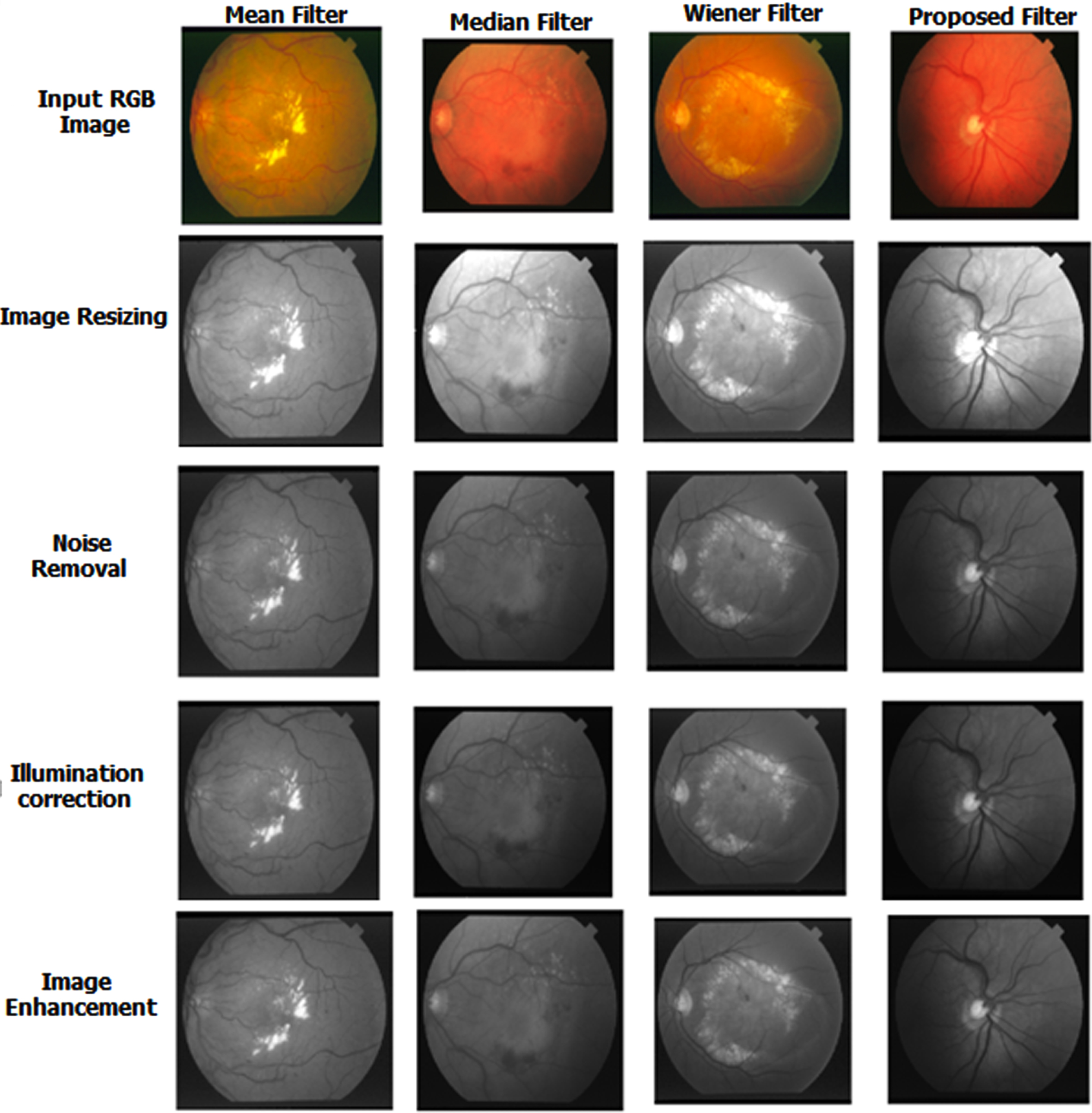
Result of Proposed Filter.

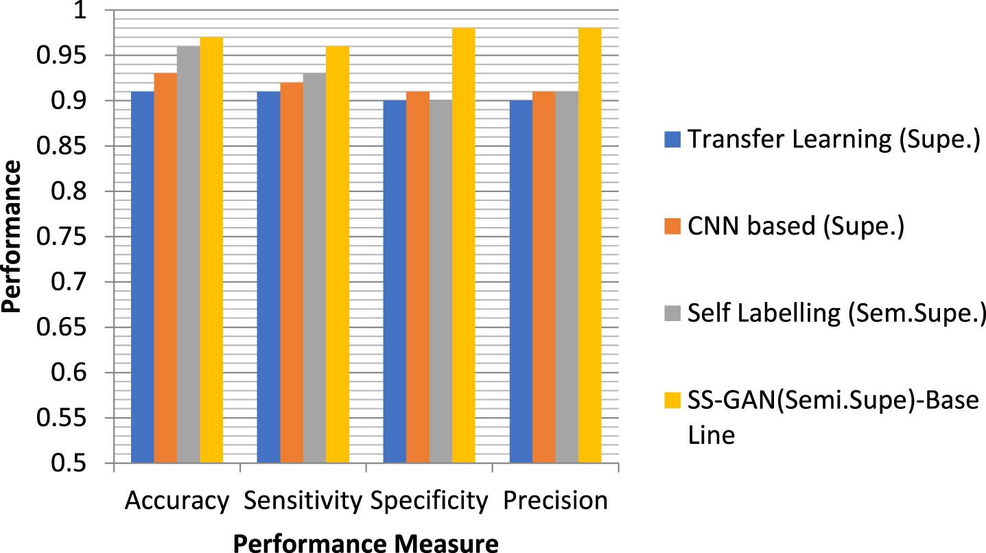
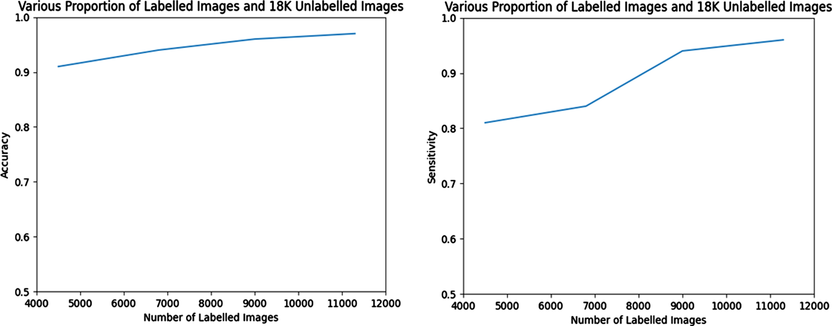
When training the semi-supervised GAN, different percentages of labelled and unlabelled pictures are used (as indicated in Table-2), respectively. On the basis of how the various ratios of the labelled and unlabelled data effect the classifier performance in semi-supervised GAN, the performance of the Semi-Supervised GAN model is compared with that of other conventional supervised classifiers. The outcomes of the experiment as determined by its several iterations are shown in Tables 2 and 3, as well as in comparison graphs.

Table 2

Performance comparison of the model (Semi-Supervised GAN) using the various proportion of labelled data

Model Training	No of labelled Images	No of un-labelled Images	Accuracy	Sensitivity	Specificity	Precision
GAN-Supervised
T1	11362	0	0.97	0.95	0.99	0.99
GAN-Semi-Supervised
T2	11362	18,000	0.97	0.96	0.98	0.98
T3	9090	18,000	0.96	0.94	0.97	0.97
T4	6817	18,000	0.94	0.85	0.82	0.81
T5	4545	18,000	0.90	0.81	0.80	0.79

Table 3

Performance comparison of the proposed model when no of labelled training image is-11362, unlabelled image is –18,000

Model	Accuracy	Sensitivity	Specificity	Precision
Transfer Learning (Supe.)	0.91	0.91	0.90	0.90
CNN based (Supe.)	0.93	0.92	0.91	0.91
Self-Labelling (Sem.Supe.)	0.96	0.93	0.9	0.91
SS-GAN (Semi.Supe)-Base Line	0.97	0.96	0.98	0.98

Table 4

Performance comparison of the model in Various Training images

Labelled Images	Accuracy		Specificity		Sensitivity		Precision
	Sup.	Sem. Sup.	Sup.	Sem. Sup.	Sup.	Sem. Sup.	Sup.	Sem. Sup.
11362	0.95	0.97	0.97	0.98	0.94	0.96	0.98	0.98
9090	0.94	0.96	0.95	0.97	0.92	0.94	0.97	0.97
6817	0.93	0.94	0.80	0.82	0.85	0.85	0.82	0.81
4545	0.89	0.91	0.80	0.81	0.81	0.81	0.79	0.79

The confusion matrix is shown in Fig. 6, which displays class 0 with a normal picture and class 1 with a glaucoma image. For the purpose of validating the suggested architecture, four distinct datasets, namely PSGIMSR, HRF, DRIONS-DB, and DRISHTI-GS, as well as merged pictures, are used. In the PSGIMSR dataset that was subjected to 10-fold cross-validation, it was determined that 470 of the Images were normal, whereas 576 of the images were aberrant. 102 of the Images have been categorised incorrectly. The performance of the proposed research is judged solely based on its results using a total of five different designs. These architectures are VGGNET-16, AlexNet, LeNet, GoogleNet, and ResNet-50. LeNet, AlexNet, GoogleNet, VGGNET-16, and ResNet-50 all obtain an accuracy of 81.07, 83.73, 86.86, and 87.04 and 88.60 respectively when using the PSGIMSR dataset. According to the conclusions of the studies, GoogleNet, VGG-16, and ResNet-50 49 perform much better than the other state-of-the-art approaches.

Strategies based on majority voting have been used in order to assess the classification’s overall success. In order to implement this method, the complete dataset was partitioned into training and testing from the outset.

Fig. 6

Performance of Semi-Supervised GAN.

In this particular research, training makes use of 70 percent of the available data, while testing makes use of the remaining 30 percent. Even while the training phase of CNN models takes a significant amount of time in general, this is not a significant factor in classification problems since the classifiers are learnt offline. In Fig. 7, we compared the amount of time needed for training various classifiers to the level of accuracy they achieved. The proposed ensemble model beats current single classifiers in terms of accuracy, while having a higher computing cost than those single classifiers. Overfitting is a fundamental problem in supervised machine learning that prevents us from perfectly generalising the models to well fit observed data on training data as well as unseen data on testing set. This is because overfitting occurs when there is too much emphasis placed on the training data. Overfitting occurs when there is noise present, there is a limit on the size of the training set, and the complexity of the classifiers used makes it difficult to generalise. This article is intended to discuss overfitting from the viewpoints of both the sources of the problem and the potential remedies to the problem. In order to mitigate the negative impacts of overfitting, a number of solutions have been suggested to address the following causes: 1) “early-stopping” is a strategy that is introduced to prevent overfitting by stopping training before the performance stops optimising; 2) “network-reduction” is a strategy that is used to exclude the noises in the training set; 3) “data-expansion” is a strategy that is proposed for complicated models to fine-tune the hyper-parameters sets with a great amount of data; and 4) “regularisation” is a strategy that is proposed to guarantee models.

Fig. 7

Performance Comparison of Proposed Semi-Supervised Learning Method.

Fig. 8

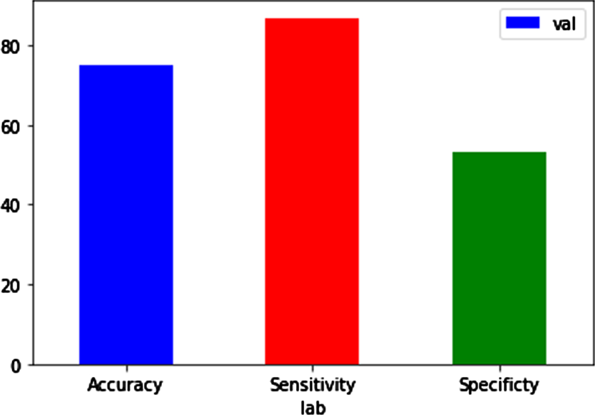
Performance metrics during validation.

The Visual Geometry Group (VGG) at the University of Oxford developed both the VGG16 and the VGG19 convolutional neural network (CNN) architectures; this is where the names “VGG16” and “VGG19” come from. VGG stands for “Visual Geometry Group.” The number of layers that are included inside the network is the fundamental distinction between these two models:

Table 5

Validation parameters

Accuracy (%)
Learning Rate	Early	Moderate	Deep	OHT
0.00001	65	60	58	75
0.0001	90	85	85	90
0.001	97.7	96	98	98
0.01	88	87	77	65

Table 6

Performance metrics of proposed work

Network	Accuracy	Sensitivity	Specificity	AUC
VGG16	0.86	0.87	0.85	0.9282
ResNet50	0.7	0.8	0.46	0.61
InceptionV3	0.77	0.87	0.54	0.63
MobileNetV2	0.63	0.63	0.62	0.65
DenseNet	0.67	0.55	0.42	0.7763
EffB0	0.79	0.97	0.38	0.77

Fig. 9

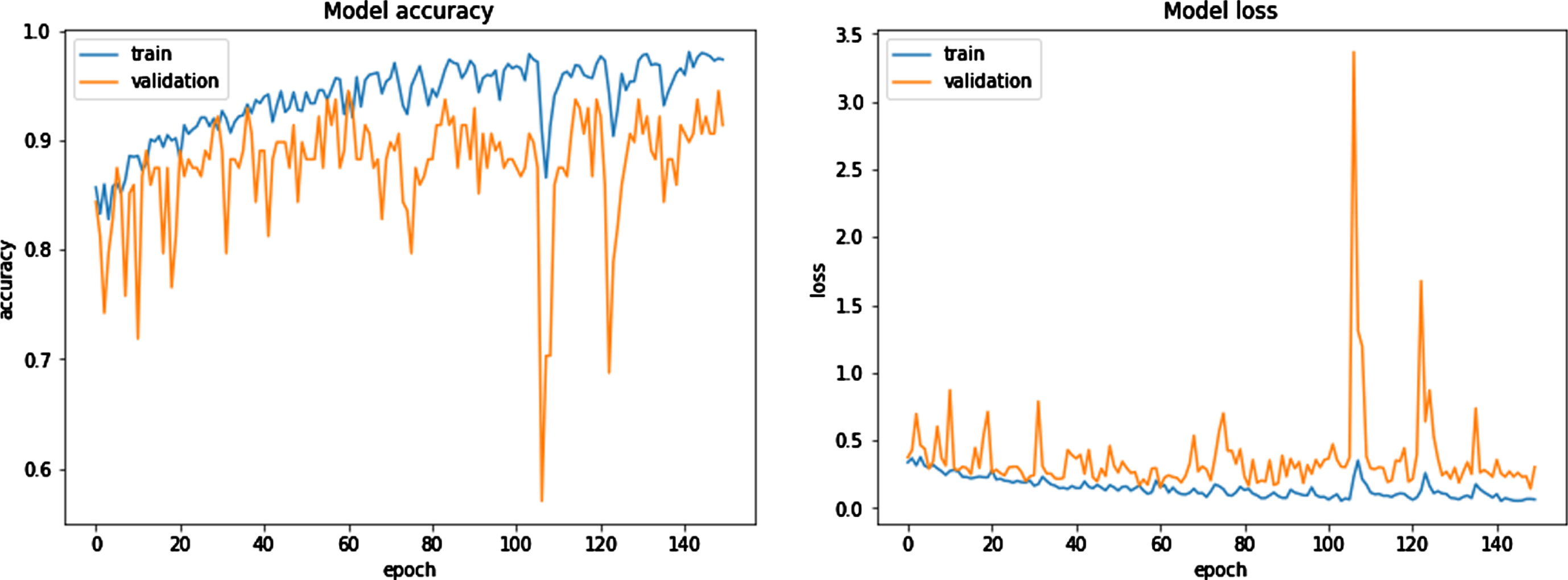
Model Accuracy Model Loss.

1. VGG16: This model’s design is comprised of a total of 16 weight layers. These consist of 13 layers of convolutional processing and 3 levels of fully linked processing. The convolutional layers make use of tiny filters measuring 3×3, whereas the network as a whole employs maximum pooling layers measuring 2×2. After many of the convolutional layers come the five max-pooling layers, which are the last layers.

2. The VGG19 model is one that is comparable to the VGG16 model, but it consists of 19 weight layers. It consists of 16 layers of convolutional processing and 3 levels of fully linked processing. It employs modest 3×3 filters in the convolutional layers, same as VGG16, and maximum 2×2 pooling layers. In addition to that, it contains five levels of maximum pooling.

Both of these networks are based on the same fundamental concept, which is that it is possible to simulate the effect of larger receptive fields (such as 5×5 or 7×7) by employing many layers that contain small filters. However, this can be accomplished with fewer parameters and with a lower level of computational complexity. VGG19 may be somewhat more accurate on certain datasets as a result of the extra layers it contains; but, it is also more computationally costly and takes more memory to execute, which might be a drawback in contexts where resources are limited. In general, the difference in overall performance that may be seen between VGG16 and VGG19 is not very large.

Note that both VGG16 and VGG19 tend to be less efficient than some later models such as ResNet, DenseNet, or EfficientNet, which use different techniques to reduce the number of parameters and the computational complexity while maintaining or improving accuracy. Specifically, ResNet, DenseNet, and EfficientNet all use ResNet as their base model.

Our statistical power may have been impacted as a result of the relatively small size of our research sample, which is one of the limitations of this particular investigation. However, the model was tested using AUC for cross validation, and as a result, our classification approach ought to be accurate enough to identify glaucoma patients with an Median range of (11.7, 3) dB.

5 Conclusion

Tuckey’s loss function is used owing to the fact that it is resistant to the effects of outliers. The suggested study has a number of advantages, the most important one being in terms of the inter-dataset performance. Experiments with around 38000 photographs showed that the algorithm had an accuracy of 98.83% across the board when applied to low-quality images from the AIIMS community camp. In addition to this, it is suggested to use a generative adversarial network (GAN) to segment the optic disc, with the adversarial and segmentation losses being properly controlled. In order to evaluate the model’s potential to generalise, it was tested on a diverse collection of datasets, including six that were publicly available and one that was kept secret. We were able to acquire an average dice score of 97.31 and 95.12 on the Drishti-GS and Refugee public datasets, respectively. This metric takes into account a wide variety of retinal artefacts, such as PPA and disc haemorrhage, as well as imaging artefacts, such as non-uniform lighting, blurring, and lens dust, among other things. Stereo pictures, which include the retina being photographed from a variety of angles, as well as optical coherence tomography (OCT) images, may also be used to investigate a depth factor in addition to two-dimensional retinal images. In stereo photography, two separate but identical Images of the same subject are taken using two different locations of the fundus camera. This gives the resulting image an impression of depth. In addition to this, the OCT pictures provide a three-dimensional image, in which the depth value of the optic cup may be found along the third dimension. It helps to provide a more accurate calculation of the cup margin, since the visibility of vessel bends improves when seen in a three-dimensional picture. Using a huge volume of clinical picture information allows for a more accurate association to be drawn between RNFL loss and glaucoma. In addition, the identification of peripapillary atrophy may be enhanced by zone- or sector-wise labelling, which indicates the degree of the extent of the atrophy, ranging from mild to severe. In addition, the severity of glaucoma may be determined by classifying patients according to alpha and beta PPA categories. A method for the automated identification and diagnosis of DR and glaucoma has been developed as a result of the work described in this thesis. Additionally, the system examined the influence of glaucoma in DR photographs in order to prevent diabetic patients from experiencing visual loss at an early stage. The following are some ways in which the suggested system may be improved in the near or distant future: (The suggested system in this thesis will be developed as a mobile application that is both user-friendly and capable of capturing retinal pictures, after which the findings of the diagnostic will be shown. (Using retinal imaging, this line of study might be expanded to identify and diagnose additional retinal illnesses, such as age-related macular degeneration and cardiovascular disease. (The proposed method for the identification and diagnosis of diabetic retinopathy and glaucoma will be able to be applied to a large collection of real-time retinal pictures of diabetic patients. (The approach has the potential to be developed to anticipate any eye-related problems even in people who do not have diabetes at an extremely early stage.

Disclosures

No, “The authors declare no conflict of interest.”