Improved graph representation learning based on neighborhood aggregation and interaction fusion

Abstract

The adaptive fusion module with an attention mechanism functions by employing a dual-channel graph convolutional network to aggregate neighborhood information. The resulting embeddings are then utilized to calculate interaction terms, thereby incorporating additional information. To enhance the relevance of fusion information, an adaptive fusion module with an attention mechanism is constructed. This module selectively combines the neighborhood aggregation and interaction terms, prioritizing the most pertinent information. Through this adaptive fusion process, the algorithm effectively captures both neighborhood features and other nonlinear information, leading to improved overall performance. Neighborhood Aggregation Interaction Graph Convolutional Network Adaptive Fusion (NAIGCNAF) is a graph representation learning algorithm designed to obtain low-dimensional node representations while preserving graph properties. It addresses the limitations of existing algorithms, which tend to focus solely on aggregating neighborhood features and overlook other nonlinear information. NAIGCNAF utilizes a dual-channel graph convolutional network for neighborhood aggregation and calculates interaction terms based on the resulting embeddings. Additionally, it incorporates an adaptive fusion module with an attention mechanism to enhance the relevance of fusion information. Extensive evaluations on three citation datasets demonstrate that NAIGCNAF outperforms other algorithms such as GCN, Neighborhood Aggregation, and AIR-GCN. NAIGCNAF achieves notable improvements in classification accuracy, ranging from 1.0 to 1.6 percentage points on the Cora dataset, 1.1 to 2.4 percentage points on the Citeseer dataset, and 0.3 to 0.9 percentage points on the Pubmed dataset. Moreover, in visualization tasks, NAIGCNAF exhibits clearer boundaries and stronger aggregation within clusters, enhancing its effectiveness. Additionally, the algorithm showcases faster convergence rates and smoother accuracy curves, further emphasizing its ability to improve benchmark algorithm performance.

1 Introduction

In the real world, there exists a significant amount of relational data that lacks a hierarchical structure. Examples of such data include transportation routes between towns, citation relationships between papers, and purchase relationships between goods. To store and analyze this data, it is represented as graphs in computer systems. Graph data is characterized by complex structures and diverse attribute types, making it suitable for learning tasks in various fields. However, as the size of graphs increases, the high dimensionality and sparsity of the data become more pronounced. To fully leverage the advantages of graph data, a data representation method called graph representation learning has emerged. The primary objective of graph representation learning is to preserve the content and structural information of nodes in the graph. This method aims to learn low-dimensional, dense, and real-valued vector representations of nodes, which can efficiently support downstream tasks such as link prediction [1, 2], node classification [3, 4], and recommendation systems [5, 6].

Graph representation learning has gained significant attention in recent years due to its applicability in various domains such as social network analysis, recommender systems, drug discovery, and knowledge graph completion. The existing techniques for graph representation learning is discussed, and an overview of their strengths, limitations, and potential applications is provided.

GCNs: Popular techniques for graph representation learning. Extend CNNs to graph-structured data by aggregating neighborhood information. Limited scalability and struggle with long-range dependencies in large graphs. GraphSAGE: Scalable approach for graph representation learning. Samples and aggregates features from a node’s local neighborhood to construct node embeddings. May lose important global information in the process of local aggregation. GAEs: Unsupervised models aiming to reconstruct the input graph. Consist of an encoder and decoder. Capture both local and global structural information. Effective in anomaly detection and link prediction tasks. Heavy reliance on reconstruction loss, may not be suitable for tasks requiring more expressive node embeddings. GATs: Utilize attention mechanisms to learn node embeddings. Assign importance weights to neighbor nodes based on relevance to the target node. Capture local and global dependencies, adaptively aggregate information, and handle graphs of varying sizes and structures. Computationally expensive training, especially for large graphs. GNNs: Diverse family of models for graph representation learning. Propagate information using graph convolutional layers. Capture complex relationships, learn expressive node embeddings, and handle diverse graph structures. Expressive power relies on network depth, challenging to train deep GNNs due to vanishing gradient problem.

Graph representation learning has witnessed significant advancements in recent years, with various techniques proposed to capture the structural information of graphs effectively. Each technique has its strengths and limitations, making them suitable for different applications. Researchers continue to explore new approaches that address the limitations of existing techniques and enhance the representation learning capabilities for graphs. The choice of technique depends on the specific task requirements and the characteristics of the target graph.

2 Related work

Graph representation learning methods can be broadly divided into two categories. The first category of graph representation learning methods is based on simple neural network techniques [7, 8]. DeepWalk was the pioneering method that introduced the concept of neural networks in deep learning to this field. It treats the nodes in a graph as words and considers the sequence of nodes generated by random walks on the graph as sentences. By employing the word representation learning algorithm Word2vec, DeepWalk learns node embedding representations. On the other hand, Planetoid incorporates label information in its learning process. It predicts class labels and neighborhood contexts in the graph to enhance graph representation learning. Although these methods based on simple neural networks have demonstrated good practical results, they may not effectively capture neighborhood similarity. For example, DeepWalk and Planetoid assume that the embedding representations of adjacent nodes in a walk sequence are similar. While this assumption holds true in extreme cases with a large number of walks, the algorithm becomes less efficient when the number of walks is small.

The second category of graph representation learning methods is based on graph Convolutional Neural Networks (GCNN), which includes Spatial Convolutional Neural Network (SCNN) [9], Chebyshev [10], Graph Convolutional Networks (GCN) [11], Simplifying Graph Convolutional Networks (SGC) [12]. The generalization of Convolutional Neural Networks is introduced to adapt to graph data with non-Euclidean structures [9]. They classified GCNN into two main types: (i) GCNN based on the frequency domain (also known as the spectral domain), which performs convolution operations on topological graphs in the frequency domain using the spectral theory of graphs, and (ii) GCNN based on the spatial domain, where the convolution operation is defined directly on the connection relationships of each node. Additionally, the SCNN algorithm is proposed, which aimed to replace the convolution kernel in the frequency domain with a parameterized diagonal matrix obtained through the Eigendecomposition of the Laplacian matrix. However, a drawback of the SCNN algorithm is that the number of parameters it needs to learn is proportional to the number of nodes in the graph, resulting in high computational complexity. The time complexity of the algorithm is O(N³), which can result in significant computational overhead when dealing with large graphs.

In order to reduce the computational complexity of the algorithm, researchers have conducted extensive research on simplifying graph convolution structures. A fixed convolution filter is used to fit the convolution kernel [10]. This filter models Chebyshev polynomials of order K + 1 (K is less than the number of nodes), which can greatly reduce the computational complexity. Since the matrix eigendecomposition of a matrix is computationally expensive, GCN uses a filter to model the first-order Chebyshev polynomials, further reducing the computational cost caused by matrix eigendecomposition and reducing the time complexity to O(|E|d). Through this filter, nodes can summarize node features from first-order neighbors. SGC further reduces computational complexity while ensuring good performance by removing the weight matrix between nonlinear transformations and compressed convolutional layers. The above GCNN algorithms mostly follow a fixed strategy of neighborhood aggregation, and the learned neighborhood information has locality, which often affects the algorithm’s representation learning. For example, both GCN and SGC use fixed transition probability matrices and aggregation operations.

In recent years, various neighborhood aggregation algorithms have been proposed, including GAT (graph attention networks) [13], GraphSAGE (graph with sample and aggregate) [14], APPNP (approximate personalized propagation of neural predictions) [15]. The GAT algorithm introduces the concept of attention mechanism in GCNN to assign different importance weights to each node and uses these learned weights to aggregate node features. GraphSAGE improves upon the neighbor sampling and aggregation methods of GCN. It changes the sampling neighborhood strategy from the entire graph to node-centered small-batch node sampling and extends the neighborhood aggregation operation by utilizing element averaging or addition, Long Short-Term Memory (LSTM), and pooling methods to aggregate neighborhood node characteristics. These methods only consider nodes within a few propagation steps, and expanding the size of the utilized neighborhood becomes challenging. The relationship between GCN and PageRank is studied and an improved propagation scheme is proposed it is corresponding algorithm, APPNP [15]. APPNP decouples the prediction and propagation processes through adjustable transmission probabilities without introducing additional parameters α, balancing the preservation of local information or utilization of large-scale neighbor information. Although these algorithms have demonstrated good performance, they do not benefit from deep models as adding layers can lead to oversmoothing issues, thus they primarily focus on building shallow models.

In order to address the issue of oversmoothing, several algorithms have been proposed, including JKNet (graphs with jumping knowledge networks) [16], GCNII (graph convolutional network with initial residual and identity mapping) [17], DeepGWC (deep graph wavelet convolutional neural network) [18]. There are differences in the range of neighborhood information of embedded nodes [16]. In response to this problem, JKNet sequentially models the neighborhood aggregation information at each level and combines them through various aggregation methods (such as connection, maximum pooling, LSTM, etc.) to achieve better structure-aware representation. GCNII adds an identity mapping by incorporating the Identity matrix into the weight matrix, in addition to using an initial residual connection. These two techniques prevent oversmoothing and improve algorithm performance. Chen et al. theoretically demonstrate that GCNII can represent a K-order polynomial filter with arbitrary coefficients, effectively aggregating K-order neighborhood features. DeepGWC improves the construction scheme of the static filtering matrix in graph wavelet neural networks by combining Fourier basis and wavelet basis. It also incorporates residual connections and an identity mapping to achieve better deep information aggregation. Although the aggregated features generated by these algorithms effectively reflect neighborhood similarity and demonstrate good practical results, there is still untapped deep-seated information in the graph data. Accessing this neighborhood information can help improve the algorithm’s performance in downstream tasks.

One of the main limitations of traditional GCNs is their limited receptive fields. This means that nodes can only directly interact with their immediate neighbors in the graph. As a result, GCNs may struggle to capture global dependencies and long-range relationships between nodes. This limitation can lead to suboptimal performance in tasks that require considering information from distant nodes or capturing complex patterns that span across the graph.

For example, in recommendation systems, where the goal is to predict user preferences based on the interactions between users and items, the ability to capture global dependencies is crucial. A user’s preferences may be influenced by the preferences of other users who are not directly connected to them but share similar interests. Traditional GCNs may fail to capture these indirect relationships, resulting in less accurate recommendations.

Similarly, in social network analysis, accurately predicting the influence or behavior of individuals requires capturing the influence patterns that extend beyond immediate connections. For instance, identifying influential users or predicting the spread of information in a social network relies on capturing global dependencies. If a GCN cannot effectively capture these long-range relationships, the predictions may be limited in their accuracy and usefulness.

By introducing the adaptive information refinement mechanism, AIR-GCN addresses these limitations and enhances the performance of GCNs in real-world applications. The attention mechanism allows the network to selectively focus on important nodes and capture global information, enabling more accurate predictions and better representation learning. The residual connections further aid in optimizing the network and retaining valuable information throughout the layers.

The limitations of traditional GCNs, such as limited receptive fields and an inability to capture global dependencies, can impact the performance of graph-based models in practical applications. AIR-GCN’s ability to address these problems makes it a valuable contribution, improving the accuracy and effectiveness of GCNs in various domains.

AIR-GCN (Adaptive Information Refinement Graph Convolutional Network) enhances the performance of graph convolutional networks (GCNs) by adaptively refining node representations through iterative information propagation. The architecture of AIR-GCN consists of multiple graph convolutional layers, each followed by a non-linear activation function. These layers form the core of the network and are responsible for learning node representations by aggregating and propagating information from neighboring nodes in the graph. However, traditional GCNs suffer from limited receptive fields, which restricts their ability to capture global information and leads to suboptimal performance.

To address this limitation, AIR-GCN introduces an adaptive information refinement mechanism. It incorporates an attention mechanism that assigns importance weights to neighboring nodes based on their relevance to the target node. This attention mechanism enables the network to selectively focus on important nodes and effectively integrate global and local information. By adaptively refining the node representations, AIR-GCN improves the model’s ability to capture complex patterns and dependencies in the graph.

Furthermore, AIR-GCN employs residual connections between graph convolutional layers. These connections allow the network to retain and propagate information from earlier layers, ensuring the preservation of valuable information throughout the network. This architecture promotes the flow of information and gradients, facilitating better optimization and learning in deep networks.

The functionality of AIR-GCN can be summarized as follows: it enhances the representation learning capabilities of GCNs by introducing an attention-based adaptive information refinement mechanism. This mechanism enables the network to better capture global dependencies and complex patterns in the graph structure. The residual connections further improve the optimization process and facilitate the flow of information throughout the network.

In order to capture nonlinear information that was previously overlooked in the graph, AIR-GCN incorporated neighborhood interaction into its modeling approach for the first time [19]. It introduces a modeling strategy that considers both neighborhood aggregation information and neighborhood interaction information. This strategy is implemented within an end-to-end framework, which exhibits excellent feature learning capability. However, the AIR-GCN algorithm suffers from several issues that can result in poor performance of the learned node embedding representation in downstream tasks:

When fusing neighborhood aggregation terms and neighborhood interaction terms, AIR-GCN employs residual learning to connect and add these two information sources [20]. However, this approach overlooks the varying importance of the two neighborhood information items for subsequent tasks.

During the AIR-GCN learning process, the failure to consider the high entropy prediction probability can impact the node embedding representation, leading to insufficient consistency of node features within local neighborhoods.

Since AIR-GCN uses the same graph data and obtains three sets of prediction probabilities through three graph convolution channels, there may be a lack of independence between the predicted outputs of each graph convolution channel, resulting in insufficient differentiation between the generated embedded representations.

Several recent papers have explored the applications and advancements of Graph Convolutional Networks (GCNs) in various domains. In 2022, “Graph Convolutional Networks with Aggregated Attention for Breast Cancer Metastasis Classification” is presented in IEEE Access [21]. Their work focused on using GCNs with an aggregated attention mechanism to improve the classification of breast cancer metastasis.

“Hierarchical Graph Convolutional Network for Semi-Supervised Node Classification,” is featured in IEEE Transactions on Neural Networks and Learning Systems [22]. Their research introduced a hierarchical approach that leveraged GCNs for semi-supervised node classification tasks.

In the field of intelligent transportation systems, “Deep Graph Convolutional Networks for Traffic Speed Prediction” is introduced in IEEE Transactions on Intelligent Transportation Systems [23]. Their work showcased the application of GCNs to predict traffic speed, providing valuable insights for traffic management and optimization.

A paper called “Graph Convolutional Networks with Relation-Aware Attention Mechanism for Traffic Flow Forecasting” is published in the same journal, IEEE Transactions on Intelligent Transportation Systems [24]. Their work proposed a GCN model with a relation-aware attention mechanism to forecast traffic flow, enhancing the accuracy of traffic predictions.

Moving into 2023, “Graph Convolutional Networks for Text Classification with Multi-Granularity Information” is published in Information Processing & Management [25]. Their research focused on utilizing GCNs to improve text classification tasks by incorporating multi-granularity information.

These papers collectively demonstrate the diverse applications of GCNs and their effectiveness in domains such as medical analysis, transportation systems, and natural language processing. They contribute to the growing body of research on GCNs and highlight their potential for solving complex problems in various fields.

Dynamic Affinity Graph Construction for Spectral Clustering Using Multiple Features was published in the IEEE Transactions on Neural Networks and Learning Systems in 2018 [26]. The paper introduces a novel approach for constructing affinity graphs in the context of spectral clustering. Spectral clustering is a popular technique for unsupervised learning that leverages the eigenvalues and eigenvectors of the graph Laplacian matrix. The authors propose a dynamic affinity graph construction method that incorporates multiple features to enhance the clustering performance. By considering multiple features, they aim to capture different aspects of the data and improve the discriminative power of the resulting clusters.

In response to the problems existing in the AIR-GCN algorithm, this paper proposes a neighborhood aggregation and interaction graph convolutional network adaptive fusion (NAIGCNAF). Let’s provide a clear problem statement, research objectives, and highlight the novelty and potential applications of our proposed solution, NAIGCNAF.

Traditional GCNs have limitations in terms of limited receptive fields and capturing global dependencies, leading to suboptimal performance in practical applications. There is a need for an improved architecture that can overcome these limitations and enhance GCNs’ representation learning capabilities. In the paper, (1) Develop a novel architecture to address the limitations of traditional GCNs, specifically limited receptive fields and the inability to capture global dependencies. (2) Propose an adaptive information refinement mechanism to selectively focus on important nodes and effectively integrate global and local information. (3) Enhance the optimization process and information flow in deep networks by utilizing residual connections between graph convolutional layers. (4) Evaluate the performance of the proposed NAIGCNAF architecture on various graph-based tasks, comparing it to traditional GCNs and other state-of-the-art models. (5)Analyze the impact of the adaptive information refinement mechanism on the model’s ability to capture complex patterns and dependencies in different domains.

Our proposed solution, NAIGCNAF, introduces the adaptive information refinement mechanism to enhance the representation learning capabilities of GCNs. This mechanism allows the network to selectively focus on important nodes and capture global dependencies, leading to improved node representations. Additionally, the incorporation of residual connections promotes better optimization and information flow in deep networks. NAIGCNAF has the potential to improve the performance of graph-based models in various domains. Some potential applications include: (1) Recommendation systems: Enhancing the accuracy of recommendations by capturing global dependencies and indirect relationships between users and items. (2) Social network analysis: Improving the prediction of influence patterns and the spread of information by capturing long-range relationships in social networks. (3) Bioinformatics: Enhancing the understanding of biological networks and predicting protein-protein interactions by capturing complex dependencies. (4) Knowledge graph analysis: Improving representation learning in knowledge graphs to enhance tasks such as entity classification and link prediction.

NAIGCNAF introduces an adaptive information refinement mechanism, which enables the network to selectively focus on important nodes and capture global dependencies effectively. By adaptively aggregating features from neighboring nodes based on their importance, NAIGCNAF overcomes the limited receptive fields of traditional GCNs. This mechanism allows the model to capture long-range relationships and complex patterns that span across the graph, significantly enhancing the representation learning process.

In addition to the adaptive information refinement mechanism, NAIGCNAF incorporates residual connections between graph convolutional layers. These connections facilitate better optimization and information flow in deep networks, enabling the model to retain valuable information throughout the layers and make more accurate predictions.

By addressing the limitations of traditional GCNs, NAIGCNAF offers several anticipated benefits. Firstly, it improves the accuracy of predictions in tasks that require capturing global dependencies, such as recommendation systems and social network analysis. Secondly, it enhances the representation learning capabilities in domains where complex patterns and long-range relationships are crucial, such as bioinformatics and knowledge graph analysis. Lastly, NAIGCNAF provides a more comprehensive understanding of the underlying structure of graphs and enables better decision-making based on the learned representations.

The proposed NAIGCNAF architecture introduces an adaptive information refinement mechanism and residual connections to enhance the representation learning capabilities of GCNs. By addressing the limitations of traditional GCNs, NAIGCNAF enables the model to capture global dependencies, retain valuable information, and make more accurate predictions. The anticipated benefits encompass improved accuracy in recommendation systems and social network analysis, enhanced representation learning in bioinformatics and knowledge graph analysis, and a deeper understanding of graph structures for better decision-making.

The main contributions of this article are summarized as follows:

The attention mechanism has been widely applied in the study of graph neural networks, serving as a core component for selecting information that is more critical to the current task goal from numerous sources. Taking inspiration from this, an attention mechanism has been incorporated into the fusion module. This addition introduces parameters that prioritize label information during the information fusion process. It enables the model to adaptively learn the attention values of neighborhood information items, and through weighted fusion, obtain an embedding representation that is better suited for downstream tasks. By implementing this scheme, the relationship between deep-level information fusion methods and node representations is established.

Introduce consistency regularization loss and difference loss in the objective function. The loss of consistency regularization can limit the prediction of low entropy output in graph convolution channels, improve the consistency of neighboring nodes, and thus improve the performance of the algorithm in node classification tasks. Differential loss imposes independence restrictions on channels to compensate for the lack of diversity between embedded representations.

The experimental results on three publicly available classic datasets demonstrate the effectiveness of the NAIGCNAF algorithm, and the NAIGCNAF framework effectively improves the performance of the benchmark image convolution algorithm in node classification tasks.

3 Materials and methods

We provide more intuitive and conceptual explanations where possible.

-Adaptive Fusion Module:

The adaptive fusion module in AFAI-GCN focuses on refining the node representations by selectively aggregating information from neighboring nodes. Think of this as a group discussion, where each node in the graph represents a participant. The adaptive fusion module enables each participant to listen carefully to others and only pay attention to the most important and relevant information that helps them in making decisions.

-Attention Mechanism:

The attention mechanism plays a crucial role in the adaptive fusion module. Intuitively, you can think of it as a spotlight that allows each participant to focus on the most relevant and informative participants in the group discussion. By incorporating label information, the attention mechanism helps the participants understand which other participants are more important for achieving the task at hand. This way, the participants can assign higher attention to the most relevant information and disregard less important information.

-Label Information:

Label information provides guidance and helps the model understand the significance of different nodes in relation to the target task. In a social network analysis scenario, label information can represent the characteristics or behaviors of individuals in the network. For example, in a recommendation system, label information can be the user preferences or item attributes. By incorporating this label information, AFAI-GCN can more effectively identify relevant nodes and capture their influence on the target node.

-Adaptive Information Refinement:

The adaptive information refinement mechanism in AFAI-GCN allows the model to adjust and improve the node representations based on the importance and relevance of neighboring nodes. It is similar to a collective decision-making process, where the participants refine their opinions by considering the opinions of others who are more knowledgeable or influential. This mechanism enables AFAI-GCN to capture long-range relationships and complex patterns that span across the graph, enhancing its representation learning capabilities.

3.1 Background knowledge

Definition 1 (Attribute Graph): The attribute graph is represented as G = (V , A , X) , where V is the node set and A ∈ R ^n ×N is a Adjacency matrix, A _i ∈ R ^n ×D represents the connection situation of node i, with element values of {0,1}. A _ij  = 1 indicates a connection between node i and node j, while A _ij  = 0 indicates no connection between node i and node j. X ∈ R^{n × D} is the attribute matrix, X _i ∈ R ^n ×D represents the attributes of node i, n represents the total number of nodes in the graph, and d represents the attribute dimension.

Definition 2 (Residual Learning): Residual learning refers to adding shortcuts between two layers of a neural network, which can alleviate the problem of gradient vanishing and dispersion in error backpropagation [27]. The residual network utilizes skip connections to linearly stack the input data and its nonlinear transformations, which helps to inject lower order features into the learning process of higher-order features and detach the algorithm from local optima. The feature of residual learning is represented as h(x), and its formula is shown in equation: $h\left(x\right)=f\left(x\right)+x$(1)

Wherein, f(x) represents the embedded features of the current hidden layer, and x represents the input feature representation.

Definition 3 (Neighborhood Aggregation): Neighborhood aggregation is the embedding representation of a node by summarizing the feature information of nodes in its local neighborhood. The necessary prerequisite for aggregating neighborhood features is neighborhood similarity, which refers to the fact that interconnected nodes should be similar, that is, the embedded representations of nodes and their neighboring nodes should be similar [28]. Therefore, the GCNN algorithm utilizes the connections between nodes to propagate feature information, ensuring that the similarity of nodes in the embedded space is similar to that of nodes in the original network.

Figure 1 describes the process using a neighborhood aggregation of node A as an example. First, input an attribute graph, use the weight matrix to perform Affine transformation on the attributes of all nodes, and map them from the original network space to the new embedded space (this process generally involves the reduction of attribute dimensions); Then, using the structural information of the graph, determine the first-order neighborhood node set of node A , where the first-order neighbor node set of node A is {A, B, C, D} ; Use the embedded representations of these nodes for weighted summation to obtain the embedded representation of node A regarding neighborhood aggregation; Determine whether to perform nonlinear transformation based on subsequent tasks.

Fig. 1

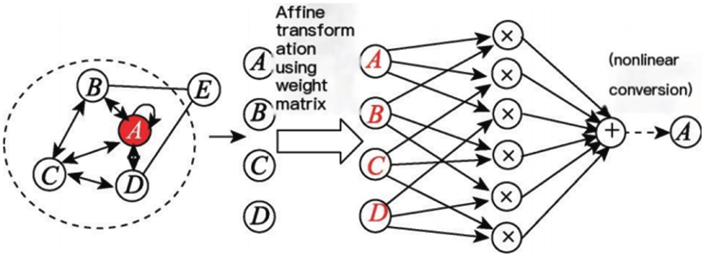
Model neighborhood aggregation terms.

Definition 4 (Neighborhood Interaction): Neighborhood interaction is the embedding representation of a node by summarizing the mutual influences of nodes in its local neighborhood. Adding neighborhood interaction calculation during the training process can help the algorithm obtain more nonlinear information in the graph [19].

Figure 2 depicts the process of node A performing a neighborhood interaction calculation as an example. Firstly, input an attribute graph and use a weight matrix to affine the node’s attributes from the original network space to the embedding space; Then determine the set of first-order neighbor nodes {A, B, C, D} of node A , multiply the embedding representations of these nodes by every two sets of elements, calculate the mutual influence between neighboring nodes, and obtain 6 neighborhood mutual influence factors; Using these 6 information items for weighted summation, obtain the embedded representation of node A regarding neighborhood aggregation; The final embedded representation can undergo nonlinear transformation based on subsequent tasks.

Fig. 2

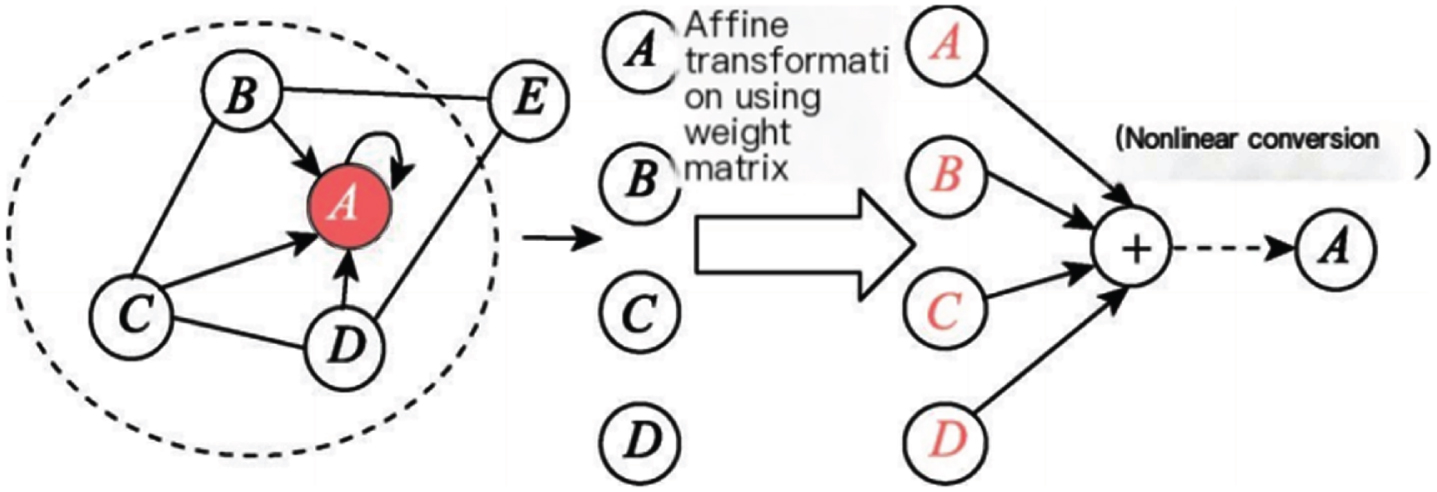
Model neighborhood interaction terms.

3.2 Algorithm description

In order to achieve more efficient information fusion, improve the performance of the classifier, and ensure that each channel obtains information relatively independently, this paper introduces the concepts of neighborhood aggregation and neighborhood interaction, and designs an adaptive graph convolutional network NAIGCNAF that integrates neighborhood aggregation and neighborhood interaction. Its overall framework is shown in Fig. 3. After inputting the data into the graph convolutional network channel, different colors represent different vector representations.

Fig. 3

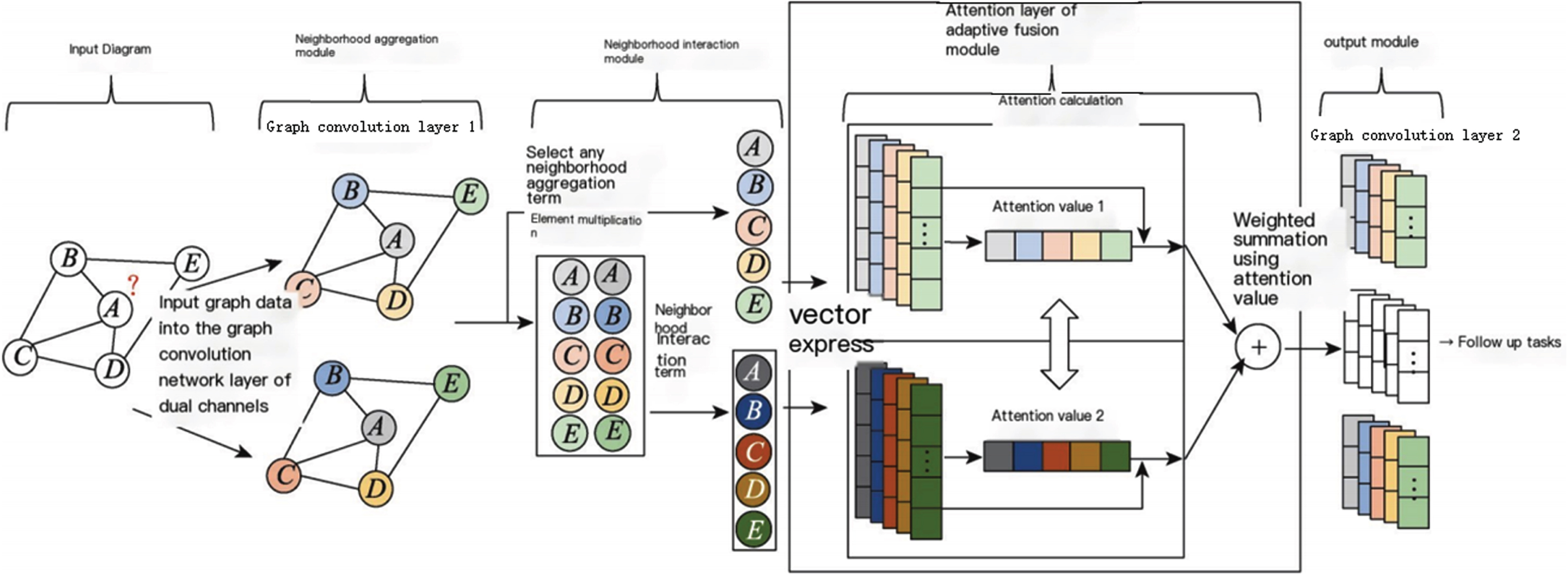
Framework of NAIGCNAF.

The algorithm takes attribute maps as input data. The neighborhood aggregation module utilizes a dual-channel graph convolutional layer to aggregate the features of neighboring nodes and generate node embedding representations, producing two distinct neighborhood aggregation terms. The neighborhood interaction module uses these two aggregation terms to perform element-wise multiplication at corresponding positions, calculating the interaction between neighborhoods and obtaining the neighborhood interaction term. One of the previously mentioned neighborhood aggregation terms, along with the neighborhood interaction term, is then selected and input into the adaptive fusion module. The adaptive fusion module incorporates an attention mechanism, which incorporates label information into the learning process of the algorithm. It calculates attention weights for the neighborhood aggregation and interaction terms separately, performs weighted fusion of these attention weights, and obtains the fused representation of neighborhood aggregation and interaction information. Finally, the output module employs a three-channel graph convolutional layer to summarize the feature information of nodes in the second-order neighborhood and outputs three sets of prediction probabilities.

For each additional layer in graph convolution, nodes aggregate higher-order neighborhood information. However, unlike the layer structure in CNN (convolutional neural networks), graph convolution cannot be deeply stacked. Li et al.’s research indicates that GCN achieves optimal performance in subsequent tasks by aggregating features from first-order and second-order neighborhoods using learned node representation vectors [29]. Stacking multiple graph convolution layers can lead to “oversmoothing,” where the node representation vectors become overly consistent. The neighborhood interaction term measures the mutual influence between two neighborhood aggregation terms, and it requires the use of dual-channel graph convolutional layers to learn these two terms separately. Therefore, in the algorithm framework of NAIGCNAF, two graph convolutional network channels were constructed, with each channel containing two graph convolutional layers.

The choice of element-by-element multiplication as the vector operation for calculating mutual influences between two neighborhood aggregations in the neighborhood interaction module of NAIGCNAF is deliberate and based on its suitability for capturing pairwise interactions between node representations. Here’s why element-by-element multiplication is often preferred over other operations:

-Capturing Pairwise Interactions: Element-by-element multiplication allows for capturing pairwise interactions between the elements of two vectors. By multiplying corresponding elements, the resulting vector emphasizes the joint influence or compatibility between the elements. In the context of NAIGCNAF, this operation enables the model to capture and highlight the mutual influences between the representations of different nodes in the graph.

-Simplicity and Efficiency: Element-by-element multiplication is a simple and computationally efficient operation that can be easily applied to two vectors without any additional complexities. It does not involve any additional learnable parameters or complex mathematical operations. This simplicity and efficiency make it particularly appealing for graph convolutional networks, where scalability and computational efficiency are crucial.

-Non-linearity: Element-by-element multiplication introduces non-linearity to the interaction process. By emphasizing joint influences and suppressing irrelevant or conflicting influences, the operation enables the model to capture complex and non-linear interactions between node representations. This non-linearity is important for NAIGCNAF to effectively model and capture intricate relationships and dependencies in the graph.

-Symmetry: Element-by-element multiplication is symmetric, meaning that the order of the vectors being multiplied does not affect the result. This symmetry property ensures that the mutual influences between two neighborhood aggregations are symmetric and balanced, regardless of the order in which the aggregations are processed. This balance helps in capturing bidirectional relationships and avoiding any bias or asymmetry in the interaction process.

While element-by-element multiplication is a suitable operation for capturing mutual influences, it’s worth noting that other operations like element-wise addition or concatenation may be more appropriate for specific tasks or scenarios. The choice of the operation depends on the nature of the problem, the desired interactions to be captured, and the characteristics of the data. It’s always important to experiment and compare different vector operations to find the one that best captures the desired relationships and interactions in the given graph-based task and dataset.

The attention mechanism chosen for the adaptive fusion module in NAIGCNAF handles the scenario when both neighborhood aggregation terms are equally important by dynamically adjusting their weights based on their relevance and importance. This mechanism allows the model to adaptively fuse the two neighborhood aggregations, giving more weight to the more informative or relevant aggregation for each node. Here’s how it impacts the overall result:

-Relevance-based Weighting: The attention mechanism calculates attention weights for each neighborhood aggregation term based on their relevance to the target node. These attention weights reflect the importance or significance of each aggregation term for the target node’s representation. When both aggregation terms are equally important, the attention mechanism assigns similar or equal weights to both terms, ensuring a balanced contribution from each term to the final representation.

-Adaptive Fusion: The attention weights obtained from the attention mechanism are then used to linearly combine the two neighborhood aggregations. The weights determine the contributions of each aggregation term to the final representation, with higher weights indicating a stronger influence. When both terms are equally important, the attention mechanism assigns similar weights to both terms, resulting in a balanced fusion of the two aggregations.

-Enhanced Discriminability: By adaptively fusing the neighborhood aggregations based on their relevance, the attention mechanism enhances the discriminability of the learned representations. It allows the model to focus more on informative aggregation terms and suppress the influence of less relevant or noisy terms. This adaptive fusion ensures that the final representation captures the most relevant and discriminative information from the neighborhood, leading to improved performance on downstream tasks.

-Robustness to Variations: The attention mechanism’s ability to handle the scenario when both neighborhood aggregation terms are equally important also contributes to the robustness of the model. It ensures that the model does not overly rely on a single aggregation term but rather takes into account both terms in a balanced manner. This robustness helps the model handle variations in the graph structure, node connectivity, or the availability of information in different neighborhoods.

The attention mechanism in the adaptive fusion module of NAIGCNAF dynamically adjusts the weights of the neighborhood aggregation terms based on their relevance, allowing for adaptive fusion and enhanced discriminability. It ensures that both terms are considered when they are equally important, leading to a balanced and robust representation for each node in the graph.

The following section provides a detailed introduction to the four main modules: neighborhood aggregation module, neighborhood interaction module, adaptive fusion module, and output module.

3.2.1 Neighborhood aggregation module

Neighborhood aggregation refers to the generation of node feature representations by combining the feature information of adjacent nodes. It is the main step in graph convolutional layer processing of features. The neighborhood aggregation term of node i is $h_i^{\mathit{agg}}$ haggi, and its calculation process is shown in equation. $h_i^{\mathit{agg}}=\sigma \left(\sum _{j\in N_i}{e}_{\mathit{ij}}{h}_{j}W\right)$(2)

Wherein, e _ij is a scalar that represents the importance of the features of node j to node i; H _j ∈ R^{l×d _k} is the embedded representation of the j-th node; W ∈ R^{d _k ×d_k+1} is the parameter matrix; σ (·) is a nonlinear Activation function; N _i is a set containing node i itself and its first-order neighbors.

Different GCNN algorithms adopt different strategies when designing neighborhood aggregation structures. Here, we mainly introduce three methods related to neighborhood aggregation.

•The design concept of neighborhood aggregation structure in GCN is to construct the importance matrix E , so that it can reasonably reflect the influence between nodes.

First, adding self connection for each node to obtain a new Adjacency matrix $\tilde{A}$ =A+I , I is the identity matrix, making the neighborhood concept more logical; To prevent gradient explosion or dispersion during multi-layer network optimization, $\tilde{A}$ Perform normalization, i.e. $\hat{A}$ = ${\tilde{D}}^{-\frac{1}{2}}\tilde{A}{\tilde{D}}^{-\frac{1}{2}}$ , $\tilde{D}$ =D+I, limiting its element values to the range of (-1,1]. The calculation process of the neighborhood aggregation term $h_i^{\left(k\right)}$ generated by GCN in the k-th layer is shown in equation. $h_i^{\left(k\right)}=\sigma \left(\sum _{j\in N_i}{\widehat{\mathit{Ah}}}_i^{\left(k-1\right)}W\right)$(3)

Wherein, the element a _ij in $\hat{A}$ is the importance value after preprocessing, corresponding to the e _ij in Equation (2).

•SGC mainly considers how to make the algorithm simpler when designing neighborhood aggregation structures. It has been theoretically proven that when K > 1, ${\hat{A}}^{\mathrm{K}}$ acts as a low-pass filter. Therefore, it removes the nonlinear activation function in the neighborhood aggregation structure, and smoothes the graph representation only by the normalized adjacency matrix of the linearly stacked K layer and the weight matrix of the first layer. The process of generating neighborhood aggregation terms in the k-th layer of SGC by arbitrarily taking k≤K is shown in equation. $h_i^{\left(k\right)}=\{\begin{array}{c}\hfill \sum _{j\in N_i}{\widehat{\mathit{Ah}}}_i^{\left(k-1\right)},k<K\hfill \\ \hfill \sum _{j\in N_i}{\widehat{\mathit{Ah}}}_i^{\left(k-1\right)}W,k=K\hfill \end{array}$(4)

When designing neighborhood aggregation structures, GraphSAGE mainly considers expanding fixed neighborhood aggregation strategies. It learns a set of aggregation functions for each node to flexibly aggregate neighboring node features; It proposes three options for aggregation functions: element averaging or addition, LSTM, and pooling. The aggregation function is the maximum pooled neighborhood aggregation term $h_i^{\left(k\right)}$ , and its calculation process is shown in equation. $h_i^{\left(k\right)}=\max \left\{\sigma \left(h_i^{\left(k-1\right)}W+b\right),\forall j\in N_i\right\}$(5)

Wherein, Max {·} is the maximum function.

In this algorithm, the neighborhood aggregation module uses the attribute graph G=(V, A, X) as input and outputs two different neighborhood aggregation embedding representations through a dual channel graph convolutional layer. Node i generates two neighborhood aggregation terms $h_i^{\mathit{agg}}$ and ${\overline{h}}_i^{\mathit{agg}}$ through the neighborhood aggregation module, the calculation process is shown in equation. $\{\begin{array}{c}\hfill h_i^{\mathit{agg}}=\sigma \left(\sum _{j\in N_i}\hat{A}{X}_{j}W\right)\hfill \\ \hfill {\overline{h}}_i^{\mathit{agg}}=\sigma (\sum _{j\in N_i}\hat{A}{X}_j{W}^{\prime }\hfill \end{array}$(6)

Wherein, σ is select function of the ReLU(x)=max (0, x).

The GCN layer structure is selected as the network structure of the neighborhood aggregation module in our algorithm and a graph convolutional network framework is constructed with strong applicability. Most improved algorithms for GCN layer structure are compatible with the framework proposed in this article.

3.2.2 Neighborhood interaction module

Neighborhood interaction refers to generating feature representations of nodes by combining the mutual influences of nodes in local neighborhoods. The mutual influence of modeling neighborhoods can enable the algorithm to obtain deep level nonlinear information in some graphs.

The neighborhood interaction module inputs two existing neighborhood aggregation terms $h_i^{\mathit{agg}}$ and ${\overline{h}}_i^{\mathit{agg}}$ , element multiplication is performed on the corresponding position to obtain a neighborhood interaction embedding representation. $h_i^{\mathit{ir}}$ is used to represent the neighborhood interaction term of node i, its calculation process is shown in equation. $\begin{array}{c}{h}_i^{\mathit{ir}}=\sigma \left(\sum _{j\in N_i}\sum _{u\in N_i}{\beta }_{\mathit{ju}}(X_{j}W\right)\otimes \left(X_u{W}^{\prime }\right))\hfill \\ =\sigma \left(\left(\sum _{j\in N_i}\hat{A}{X}_{j}W)\otimes (\sum _{u\in N_i}\hat{A}(X_u{W}^{\prime }\right)\right)\hfill \\ =\sigma \left(h_i^{\mathit{agg}}\otimes {\overline{h}}_i^{\mathit{agg}}\right)\hfill \end{array}$(7)

Wherein, σ selects the Sigmaid function. β _ju is a scalar that represents the interaction weight between the neighborhood aggregation term of node j and the neighborhood aggregation term of node u. The larger the value, the more relevant information of node i is contained in the mutual influe.

The vector operations that can be selected when calculating the mutual influence between two neighborhood aggregations include adding, subtracting, multiplying, and dividing elements by element, and taking the average, maximum, and minimum values by element. This article adopts element by element multiplication, which can meet the practical needs of calculating the interactions between neighboring regions.

3.2.3 Adaptive fusion module

In order to leverage the performance advantages of residual learning, AIR-GCN incorporates skip join addition based on neighborhood aggregation terms and neighborhood interaction terms during information fusion. However, this approach overlooks the varying importance of the two information items to the task, potentially resulting in a fused embedded representation that is not optimal for subsequent tasks. To address these shortcomings, AFAI-GCN introduces an attention mechanism in the fusion module. This mechanism incorporates tag information into the fusion process, allowing for the learning of attention values for the aforementioned information items. These learned attention values are then used to conduct weighted summation, resulting in an embedded representation that effectively combines neighborhood aggregation and neighborhood interaction information.

In the adaptive fusion module, input the neighborhood interaction term $h_i^{\mathit{ir}}$ and any one of the two neighborhood aggregation terms (such as $h_i^{\mathit{agg}}$ ), and send them into the attention layer; The attention layer projects these two embedded representations into the low dimensional vector space, adds activation function for nonlinear transformation, and obtains the nonlinear embedded representation; Multiply it with a learnable attention weight vector to obtain the attention values ${\omega }_i^{\mathit{agg}}$ and ${\omega }_i^{\mathit{ir}}$ of node i regarding the neighborhood aggregation term and neighborhood interaction Term, their calculation processes are shown in equation. $\{\begin{array}{c}\hfill {\omega }_i^{\mathit{ir}}=q^T·\mathit{tanh}\left(W{\left(h_i^{\mathit{ir}}\right)}^T+b\right)\hfill \\ \hfill {\omega }_i^{\mathit{agg}}={\overline{q}}^T·\mathit{tanh}\left(W^{\prime }{\left(h_i^{\mathit{agg}}\right)}^T+b^{\prime }\right)\hfill \end{array}$(8)

Wherein, W , W ^′ ∈ R^d′×d₁ is the parameter matrix of the attention layer, b, b^′ ∈ R^d′×1 is the deviation vector, q, $\overline{q}$ ∈ R^d′×1 is the attention weight vector. Adding parameter matrices and attention weight vectors to the attention layer can control the calculation process of Equation (8) in the label information section.

Softmax function is used to measure attention values ${\omega }_i^{\mathit{agg}}$ and ${\omega }_i^{\mathit{ir}}$ performs normalization processing by limiting the range of element values to (0,1) and ensuring that the sum of the two terms is 1, resulting in normalized attention values ${\alpha }_i^{\mathit{agg}}$ and ${\alpha }_i^{\mathit{ir}}$ . Their calculation process is shown in equation. $\{\begin{array}{c}\hfill {\alpha }_i^{\mathit{ir}}=\mathit{Softmax}\left({\omega }_i^{\mathit{ir}}\right)=\frac{\mathit{exp}\left({\omega }_i^{\mathit{ir}}\right)}{\mathit{exp}\left({\omega }_i^{\mathit{ir}}\right)+\mathit{exp}\left({\omega }_i^{\mathit{agg}}\right)}\hfill \\ \hfill {\alpha }_i^{\mathit{agg}}=\mathit{Softmax}\left({\omega }_i^{\mathit{agg}}\right)=\frac{\mathit{exp}\left({\omega }_i^{\mathit{agg}}\right)}{\mathit{exp}\left({\omega }_i^{\mathit{ir}}\right)+\mathit{exp}\left({\omega }_i^{\mathit{agg}}\right)}\hfill \end{array}$(9)

When ${\alpha }_i^{\mathit{ir}}$ is greater than ${\alpha }_i^{\mathit{agg}}$ , it means that $h_i^{\mathit{ir}}$ is more important in the fusion term.

The adaptive fusion module uses the learned attention value to weighted sum the two embedded representations $h_i^{\mathit{ir}}$ and $h_i^{\mathit{agg}}$ to obtain the fusion term $h_i^{\mathit{aair}}$ of neighborhood aggregation and neighborhood interaction information. The calculation process is as shown in equation. $h_i^{\mathit{aair}}={\alpha }_i^{\mathit{ir}}*h_i^{\mathit{ir}}+{\alpha }_i^{\mathit{agg}}*h_i^{\mathit{agg}}$(10)

3.2.4 Output module

The neighborhood aggregation module is used to obtain two different neighborhood aggregation terms $h_i^{\mathit{agg}}$ and ${\overline{h}}_i^{\mathit{agg}}$ , respectively, an adaptive fusion module, is used to obtain the fusion term $h_i^{\mathit{aair}}$ as input to the output module. Create three graph convolutional layers in the output module, inject second-order neighborhood information into the three embedding representations mentioned above, and obtain low dimensional prediction probability vectors $z_i^{\mathit{agg}}$ , ${\overline{z}}_i^{\mathit{agg}}$ and $z_i^{\mathit{aair}}$ , the calculation process is shown in equation. $\{\begin{array}{c}\hfill z_i^{\mathit{agg}}=\sigma \left(\sum _{j\in N_i}{\widehat{\mathit{Ah}}}_i^{\mathit{agg}}W\right)\hfill \\ \hfill z_i^{\mathit{aair}}=\sigma \left(\sum _{j\in N_i}{\widehat{\mathit{Ah}}}_i^{\mathit{aair}}{W}^{\prime }\right)\hfill \\ \hfill {\overline{h}}_i^{\mathit{agg}}=\sigma \left(\sum _{j\in N_i}\hat{A}{\overline{h}}_i^{\mathit{agg}}\mathrm{W”}\right)\hfill \end{array}$(11)

Wherein, W, W’, W” ∈ R^d₁×d₂ is the parameter matrix, σ selects the Softmax function, which converts the multi classification results into probability form, with the category with the highest probability value as the predicted result. In the subsequent calculation process of the objective function, this probabilistic form of prediction representation is required.

3.3 Objective function

The objective function is a set of loss function that need to be optimized during the training process of the algorithm. When designing a semi supervised GCNN algorithm, the objective function not only includes the supervised loss of labeled nodes, but also typically combines the graph regularization loss to smooth the label information on the graph through regularization loss [11, 29]. The algorithm in this article has made the following improvements in the objective function section:

The prediction probability of high entropy may lead to insufficient consistency of node features within local neighborhoods. Therefore, adding information consistency constraints to the objective function can help enhance the consistency of node features within local neighborhoods and improve the performance of the algorithm in node classification tasks.

Multiple channels use the same graph data and they work in parallel, so it is necessary to consider the mutual influence between the predicted outputs of the channels. Therefore, an information difference constraint has been added to the objective function, which can impose independent constraints on the predicted output of each channel, enabling the algorithm to obtain more diverse and in-depth information.

On the basis of preserving the supervised loss, this article adds two information constraints to the objective function, which includes three terms: supervised loss, consistency regularization loss, and difference loss.

3.3.1 Supervisory losses

Three sets of prediction probabilities, $z_i^{\mathit{agg}}$ , ${\overline{z}}_i^{\mathit{agg}}$ and $z_i^{\mathit{aair}}$ , were obtained through the output module, the supervised loss is calculated using these three sets of probabilities and real data labels for differences. In order to measure the difference between the predicted probability and the real data label, this paper chooses to calculate the cross entropy loss of two sets of probability distributions as the supervision loss. Given the training set M , select any label node m ∈ M , and get the prediction probability $z_m^{\left(s\right)}$ of the corresponding node through the th channel. The cross entropy loss between it and the real data label y _m is $L_m^{\left(s\right)}$ . The calculation formula is in equation. $L_m^{\left(s\right)}=-\sum _{m\in M}\sum _{i=1}^C{y}_{\mathit{mi}}{\mathit{lnz}}_{\mathit{mi}}^{\left(s\right)}$(12)

Wherein, Z ∈ R ^{n × C} is the prediction probability of the classifier, y ∈ R ^{n × C} is the real data label, and C represents the total number of categories.

3.3.2 Consistency regularization loss

To optimize the algorithm’s performance in the classification task, it is important to prevent the decision boundary of the classifier from crossing the high-density area of the marginal distribution of the data [31]. One common approach to achieve this is to restrict the classifier’s output to low entropy predictions for unlabeled data [32]. In line with this approach, this article introduces an information consistency constraint to the objective function. This constraint helps limit the algorithm’s prediction output, reduce the average variance of its probability distribution, and generate a smoother embedding representation of the graph.

NAIGCNAF uses three graph convolutional channels, so it is necessary to expand the above approach to adapt to multi-channel structures. Firstly, equation is used to calculate the average of all prediction probabilities and obtain the center of the prediction probability. ${\overline{z}}_i=\frac{1}{S}\sum _{s=1}^S{z}_i^{\left(s\right)}$(13)

Wherein, $z_i^{\left(s\right)}$ represents the predicted output generated by node i through the s-th channel, and S represents the total number of channels. The output module of NAIGCNAF uses three channels, namely two GCN channels and one fusion information channel.

If the entropy value of the label distribution is high, it means that the learned nodes have significant differences from their neighboring features or labels, which is not conducive to expressing neighborhood similarity. Further aggregation may damage algorithm performance [28]. Therefore, after obtaining the average prediction $\overline{z}$ , Sharpen technique is used to reduce the entropy of the label distribution [32]. ${\overline{z}}_{\mathit{ij}}^{\prime }$ represents the low entropy prediction probability of node i on class j, and its calculation process is shown in equation. $\begin{array}{c}\hfill {\overline{z}}_{\mathit{ij}}^{\prime }=\mathit{Sharpen}\left(\overline{z},T\right)=\frac{{\overline{z}}_{\mathit{ij}}^{\frac{1}{T}}}{\sum _{c=1}^C{\overline{z}}_{\mathit{ic}}^{\frac{1}{T}}},\hfill \\ \hfill 0\le j\le C-1\hfill \\ \hfill \hfill \end{array}$(14)

Wherein, T is a parameter, and when T ⟶ 0, the output of Sharpen( ,T) will approach the Dirac distribution, where all values in the probability distribution are concentrated near a point. Therefore, using a lower T value will result in the algorithm outputting a prediction with lower entropy.

The Sharpen technique is a method used to reduce the entropy or uncertainty of a label distribution. It is commonly applied in scenarios where the predicted probabilities of different labels are relatively close to each other, indicating a high degree of uncertainty or ambiguity in the model’s predictions.

The basic idea behind the Sharpen technique is to accentuate or sharpen the predicted probabilities of the labels, making them more distinct and less evenly distributed. This can be achieved by applying a temperature parameter to the softmax function, which is typically used to convert the model’s output logits into probabilities.

In the softmax function, the temperature parameter (often denoted as T) controls the steepness or smoothness of the resulting probability distribution. A higher temperature value (>1) leads to a smoother distribution where the probabilities are more evenly spread, whereas a lower temperature value (<1) sharpens the distribution by amplifying the differences between the probabilities.

By using a lower temperature value, the Sharpen technique encourages the model to make more confident predictions by emphasizing the highest probability and suppressing the influence of other labels. This helps to reduce the overall entropy or uncertainty of the label distribution.

It is worth noting that the Sharpen technique should be used with caution, as excessively sharpening the distribution can lead to overconfidence and potentially degrade the model’s performance. Therefore, it is crucial to find an appropriate temperature value that balances the reduction in entropy with the model’s accuracy and reliability.

L _c is used to represent the loss of consistency regularization, which represents the square L₂ norm of ${\overline{z}}^{\prime }$ and multiple output predictions z, and the calculation process is shown in equation. $L_c=\frac{1}{S}\sum _{i=1}^n\left(\sum _{s=1}^S{\left|\left|{\overline{z}}_i^{\prime }-z_i^{\left(s\right)}\right|\right|}_2^2\right)$(15)

Wherein, $z_i^{\left(1\right)}$ , $z_i^{\left(2\right)}$ , $z_i^{\left(3\right)}$ represents three sets of prediction probabilities $z_i^{\mathit{agg}}$ , $z_i^{\mathit{aair}}$ , ${\overline{z}}_i^{\mathit{agg}}$ obtained through the output module.

3.3.3 Differential loss

This article adds an information difference constraint to the objective function, which can measure the independence between random variables and is conducive to quantifying the mutual influence between channels. The difference constraint adopts a kernel based independence metric - the Hilbert Schmidt independence criterion (HSIC).

The Hilbert Schmidt Independence Criterion (HSIC) is a statistical measure used to assess the independence between two random variables by comparing their joint distribution with the product of their marginal distributions. In the context of the mentioned implementation, HSIC is employed to ensure independence between two pairs of prediction probabilities.

The choice of the inner product kernel function is crucial in the calculation of HSIC as it defines the notion of similarity or distance between data points. The kernel function is responsible for mapping the data from the input space to a higher-dimensional feature space where the calculations are performed.

Different kernel functions can be used based on the characteristics of the data and the specific requirements of the problem. Commonly used kernel functions include the Gaussian (RBF) kernel, polynomial kernel, linear kernel, and sigmoid kernel, among others. Each of these kernel functions has its own properties and can capture different types of relationships or dependencies in the data.

The general idea of such methods is to use the cross-covariance operator defined on the reproducing kernel Hilbert space to derive statistics suitable for measuring independence and determine the size of independence [33].

Assuming that X and Y are two sets of observable variables, for x ∈ X and y ∈ Y , the mappings on the reproducing kernel Hilbert space B and Q are defined respectively Φ (x) ∈ B and Ψ (y) ∈ Q , the corresponding kernel functions are k(x, x ’) and l(y, y ’), and their calculation process is shown in equation. $\{\begin{array}{c}\hfill k\left(x,x^{\prime }\right)=〈\Phi \left(x\right),\Phi \left(x^{\prime }\right)〉,x,x^{\prime }\in X\hfill \\ \hfill l\left(y,y^{\prime }\right)=〈\Psi \left(y\right),\Psi \left(y^{\prime }\right)〉,y,y^{\prime }\in Y\hfill \end{array}$(16)

The cross-covariance operator can be expressed as C _xy : B ⟶ Q in equation. $C_{\mathit{xy}}=E_{\mathit{xy}}\left[\left(\mathit{\Phi }\left(x\right)-E_x\mathit{\Phi }\left(x\right)\right)\otimes \left(\mathit{\Psi }\left(y\right)-E_y\mathit{\Psi }\left(y\right)\right)\right]$(17)

Wherein, ⊗ represents Tensor product, E _x Φ (x) and E _y Ψ (y) Represent separately Φ (x) and Ψ (y) expectations.

HSIC calculates the empirical estimate value of the Hilbert Schmidt Cross-covariance Operator norm to obtain the independence judgment criterion, and its expression is shown in equation. $\mathit{HSIC}\left(B,Q\right)={\left|\left|{\mathit{C}}_{\mathit{xy}}\right|\right|}_{\mathit{HS}}^2$(18)

When observing data {(x₁, y₁), (x₂, y₂),..., (x _n , y _n )}, the empirical estimation value of HSIC is shown in equation. $\mathit{HSIC}\left(\mathit{X},\mathit{Y}\right)={\left(n-1\right)}^{-2}\mathit{tr}\left(\mathit{RKRL}\right)$(19)

Wherein, R  =  I - (1/n) ee ^T , I represents the Identity matrix, e is the column vector with the element value of 1, K and L are respectively the Gram matrices of the kernel k and l with respect to the observation value [34], that is, K _ij  = k( x _i , x _j ), L _ij  = l( y _i , y _j ).

Three sets of prediction probabilities z ^agg , z ^aair and ${\overline{z}}^{\mathit{agg}}$ are obtained from the output module. Since they learn from the same graph G = (V, A, X) , an information constraint term needs to be added to ensure that they can obtain different information. To this end, the differential loss L _d is added to the objective function, which is the sum of the HSIC values calculated by z ^agg , ${\overline{z}}^{\mathit{agg}}$ , and z ^aair , respectively. The calculation process is shown in equation. ${\mathit{L}}_{\mathit{d}}=\mathit{HSIC}\left(z^{\mathit{agg}},z^{\mathit{aair}}\right)+\mathit{HSIC}\left(z^{\mathit{aair}},{\overline{z}}^{\mathit{agg}}\right)$(20)

The kernel function is equivalent to the similarity between two samples. In the implementation of this algorithm, the inner product kernel function is chosen to describe this relationship, which is K  =  z · z ^T .

The empirical estimation value of HSIC has been theoretically proven, and the larger its value, the stronger the correlation between the two variables, and the closer it is to 0, the stronger the independence of the two variables [35]. Introducing this constraint can assist in optimizing the algorithm, minimizing it during the training process, improving the independence between two pairs of prediction probabilities, and helping the graph convolution channel learn its own unique information, thereby improving the difference between the two sets of embedded representations.

3.4 Optimization objectives

The overall objective function that the algorithm needs to optimize is the weighted sum of the three losses mentioned above, and the calculation process is shown in equation. $\mathit{L}=\sum _{\mathit{s}=1}^{\mathit{S}}{\mathit{k}}_{\mathit{s}}*{\mathit{L}}_{\mathit{m}}^{\left(\mathit{s}\right)}+t*{\mathit{L}}_{\mathit{c}}+r*{\mathit{L}}_{\mathit{d}}$(21)

Wherein, k _s is the weight of the supervised loss on the s-th graph convolution channel, while t and r are the weights of the consistency regularization loss and the difference loss, respectively. The algorithm utilizes labeled training samples for data learning and minimizes the objective function during backpropagation for model optimization.

In the proposed model, the overall optimization objective is defined as the weighted sum of three losses: the classification loss, the sharpening loss, and the independence loss. The choice of the weighting scheme and how the weights were determined is an important aspect of the model’s design.

The weighting scheme is typically determined based on the relative importance or priority assigned to each loss term. In other words, it reflects the desired trade-off between different objectives in the overall optimization process. The weights can be chosen based on domain knowledge, empirical evaluation, or heuristic reasoning.

The determination of the weights can be done in various ways. One common approach is to perform a hyperparameter search or grid search, where different combinations of weights are tested, and the performance of the model is evaluated on a validation set or through cross-validation. The weights that yield the best performance or achieve the desired trade-off are then selected.

Another approach is to set the weights based on prior knowledge or assumptions about the problem. For example, if one loss term is considered to be more critical or has a higher impact on the overall performance, it can be assigned a higher weight. This approach requires a deep understanding of the problem and the specific requirements of the application.

Algorithm: NAIGCNAF algorithm

Input: attribute graph G = (V, A, X) , Learning rate η, Nonlinear Activation function σ.

Output: Embedded represents z ^agg , ${\overline{z}}^{\mathit{agg}}$ , and z ^aair .

1. Initialize all weight matrices Theta

2. While algorithm does not converge:

3. For each node i ∈ V do :

4. Use Equation (6) to calculate the two first-order neighborhood aggregation terms $h_i^{\mathit{agg}}$ and ${\overline{h}}_i^{\mathit{agg}}$

5. Calculate the neighborhood interaction term $h_i^{\mathit{ir}}$ using Equation (7)

6. Use Equations (8) and (9) to calculate the attention values ${\alpha }_i^{\mathit{agg}}$ and ${\alpha }_i^{\mathit{ir}}$

7. Calculate the adaptive fusion term $h_i^{\mathit{aair}}$ using Equation (10)

8. Use Equation (11) to calculate three predicted outputs $z_i^{\mathit{agg}}$ , ${\overline{z}}_i^{\mathit{agg}}$ and $z_i^{\mathit{aair}}$

9. end for

10. Use Equation (12) to calculate the supervised classification loss L _m , use Equations (13) to (15) to calculate the consistency regularization loss L _c , and use Equation (20) to calculate the difference loss L _d

11. Based on the Adam optimizer, update all parameters Theta using Equation (21)

12. end while

13 Returns the final embedding vector z ^agg , ${\overline{z}}^{\mathit{agg}}$ , and z ^aair

3.5 Key notes

The motivation behind employing a dual-channel graph convolutional network (GCN) is to capture both local and global structural information of the graph. Existing GCN-based models typically operate on a single graph structure and may not be able to capture the complex relationships between nodes in the graph. The dual-channel GCN consists of two parallel channels, one that captures local information and the other that captures global information. The local channel uses the standard GCN operation to aggregate information from the node’s local neighborhood, while the global channel aggregates information from the entire graph using a graph pooling operation. By combining both local and global information, the dual-channel GCN can better represent the structural information of the graph and improve the performance of downstream tasks such as node classification and link prediction.

The adaptive fusion module with an attention mechanism is designed to address the limitation of existing fusion methods that may not be suitable for graphs with varying structures and characteristics. The adaptive fusion module dynamically learns the importance of each feature for each node in the graph using an attention mechanism. The attention mechanism assigns weights to the features based on their relevance to the target node, allowing the model to adaptively fuse the features to obtain a more informative representation. This approach is particularly useful for graphs with varying structures, where different features may be more relevant for different nodes. The adaptive fusion module can improve the representation learning capability of the model and enhance the performance of downstream tasks such as node classification, link prediction, and graph classification.

3.6 Attention mechanism in the adaptive fusion module

The attention mechanism in the adaptive fusion module of NAIGCNAF plays a crucial role in selectively aggregating information from neighboring nodes based on their importance and relevance to the target node. This mechanism allows NAIGCNAF to adaptively refine the node representations by focusing on informative nodes and capturing global dependencies effectively.

Incorporating label information in the learning process is essential for the attention mechanism to determine the importance of neighboring nodes. The label information provides valuable guidance and helps the model understand the significance of different nodes in relation to the target node’s task-specific objective. By leveraging this label information, NAIGCNAF can assign higher attention weights to nodes that are more relevant to the target task and suppress the influence of less informative nodes.

Specifically, the attention mechanism incorporates label information through a learnable attention weight matrix. This weight matrix is trained during the learning process and is used to compute attention scores for each neighboring node. These attention scores reflect the importance of each node in relation to the target node and are used to weight the aggregation of neighboring node features.

The attention scores are typically computed by taking into account both the features of neighboring nodes and the label information. This allows NAIGCNAF to learn a task-specific attention mechanism that captures the most relevant information from the graph for the target task. The attention mechanism can be implemented using various approaches, such as dot product attention, additive attention, or self-attention mechanisms like the Transformer model.

By incorporating label information in the attention mechanism, NAIGCNAF can effectively capture the dependencies and patterns in the graph that are most relevant to the target task. This adaptive fusion of information based on the attention mechanism enhances the representation learning capabilities of NAIGCNAF and contributes to its improved performance compared to traditional GCNs.

The attention mechanism in the adaptive fusion module of NAIGCNAF utilizes label information to determine the importance of neighboring nodes. By incorporating label information through a learnable attention weight matrix, NAIGCNAF can selectively aggregate information from informative nodes and capture global dependencies effectively. This attention mechanism plays a crucial role in enhancing the representation learning capabilities of NAIGCNAF and contributes to its improved performance in graph-based tasks.

3.7 Discuss the choice of the ReLU activation function

The choice of the ReLU activation function in the neighborhood aggregation module of NAIGCNAF is deliberate and based on its desirable properties for graph convolutional networks. Here’s why ReLU is often preferred over other activation functions:

-Non-linearity: The ReLU activation function introduces non-linearity to the network, allowing it to model complex relationships and capture non-linear patterns in the data. This non-linearity is crucial for the neighborhood aggregation module to learn and represent intricate relationships among nodes in the graph.

-Sparsity: ReLU introduces sparsity by setting negative values to zero. This sparsity property can be beneficial in graph-based scenarios where the graph structure often exhibits sparse connectivity. By setting negative values to zero, ReLU helps the model focus on positive and informative signals, filtering out noise and irrelevant information.

-Computational Efficiency: ReLU is computationally efficient to compute compared to other activation functions like sigmoid or tanh. The ReLU function simply sets negative values to zero without involving additional computations, making it faster to compute during the forward and backward propagation steps. This efficiency is particularly advantageous for large-scale graph datasets with millions or billions of nodes.

-Avoiding Vanishing Gradient: ReLU helps mitigate the vanishing gradient problem, which can occur in deep neural networks. The vanishing gradient problem refers to the phenomenon where gradients diminish exponentially as they propagate backward through layers, leading to slow convergence or even stagnation of learning. ReLU’s non-saturating nature helps alleviate this problem by allowing gradients to flow more easily during backpropagation.

-Interpretability: ReLU offers interpretability as it preserves the positive activations as they are, without any transformations or distortions. This property can be advantageous when analyzing and interpreting the learned representations or when explaining the model’s decisions.

While ReLU has its advantages, it is worth noting that different activation functions may be more suitable for specific tasks or datasets. It’s always important to experiment and compare different activation functions to find the one that best suits the requirements of the given graph-based task and dataset.

4 Experiment and performance analysis

4.1 Dataset and sample selection

All experiments were conducted on three common citation datasets, Cora (Machine Learning Citation Network), Citeseer (Conference Citation Network), and Pubmed (Biomedical Citation Network). The choice of datasets in any machine learning approach is crucial as it directly impacts the performance evaluation, generalizability, and relevance of the proposed approach. In the case of the proposed approach, the selection of Cora, Citeseer, and Pubmed datasets is likely motivated by their specific characteristics and relevance to the task at hand. Here are some justifications for the dataset selection:

-Cora (Machine Learning Citation Network): Cora dataset is a popular benchmark dataset in the field of machine learning. It consists of scientific publications related to machine learning, where each publication is represented as a bag-of-words feature vector. The dataset also includes citation links between the publications. Cora is relevant to the proposed approach as it involves predicting the categories or topics of the publications based on their textual content, which aligns with the classification task addressed in the approach.

-Citeseer (Conference Citation Network): Citeseer is another widely used dataset in the field of citation network analysis. It contains scientific publications from various conferences, where each publication is represented as a bag-of-words feature vector. Similar to Cora, Citeseer also includes citation links between the publications. This dataset is relevant to the proposed approach as it involves the classification of publications into predefined categories based on their textual content, which is similar to the task addressed in the approach.

-Pubmed (Biomedical Citation Network): Pubmed dataset is specifically focused on the biomedical domain and comprises scientific publications related to biomedical research. Each publication is represented as a bag-of-words feature vector, and citation links between the publications are included. The relevance of Pubmed to the proposed approach lies in its biomedical context, which introduces additional challenges such as specialized terminology and domain-specific knowledge. By including Pubmed, the proposed approach can demonstrate its capability to handle the specific challenges of the biomedical domain.

These datasets offer several advantages for evaluating the proposed approach:

-Standard Benchmark: Cora, Citeseer, and Pubmed are well-established benchmark datasets in the field of citation network analysis and text classification. They have been extensively used in previous research, allowing for meaningful comparisons and benchmarking of the proposed approach against existing methods.

-Real-World Relevance: These datasets are derived from real-world scientific publications, making them relevant to the tasks of document classification and citation network analysis. The proposed approach can demonstrate its effectiveness in real-world scenarios by performing well on these datasets.

-Diversity: The chosen datasets cover different domains (machine learning, conferences, and biomedical research) and exhibit varying characteristics. This diversity allows for a comprehensive evaluation of the proposed approach’s generalizability and robustness across different domains.

When selecting samples, a unified scheme is adopted. Each class randomly selects 20 labeled nodes to form a training set, 500 nodes to form a validation set, and 1000 nodes to form a test set. Table 1 shows the detailed information and sample selection of the three datasets.

Table 1

Datasets and sample selection

Data set	Cora	Citeseer	Pubmed
Node	2708	3327	19717
Edge	5429	4732	44338
Attribute	1433	3703	500
Label	7	6	3
Training	140	120	60
Verification	500	500	500
Testing	1000	1000	1000

The specific numbers of labeled nodes chosen for the training, validation, and test sets are likely determined based on various factors, including the nature of the dataset, the availability of labeled data, and the desired experimental setup. While the exact reasoning behind the specific numbers may not be explicitly mentioned, here are some possible justifications:

-Dataset Size: The size of the dataset plays a crucial role in determining the number of labeled nodes. If the dataset is large, it might be feasible to allocate a higher number of labeled nodes for training, validation, and test sets. On the other hand, with smaller datasets, it becomes necessary to carefully allocate a limited number of labeled nodes to ensure a sufficient representation of the data.

-Resource Constraints: The availability of labeled data might be limited due to various factors such as time, cost, or difficulty in obtaining annotations. In such cases, the numbers of labeled nodes for training, validation, and test sets are determined based on the available resources.

-Evaluation Requirements: The specific numbers of labeled nodes for the training, validation, and test sets might be chosen to meet specific evaluation requirements. For instance, if the proposed approach aims to evaluate its performance with limited labeled data, a smaller number of labeled nodes might be allocated for training and validation to simulate a semi-supervised learning scenario.

-Experimental Design: The allocation of labeled nodes can be influenced by the desired experimental design. For example, if the goal is to evaluate the impact of different training set sizes, a range of labeled nodes can be selected to form training sets of varying sizes, while keeping the validation and test sets fixed.

4.2 Benchmark methods and parameter settings

In the node classification experiment, the NAIGCNAF algorithm was compared with several classic graph representation learning algorithms, including two neural network models MLP (multilayer perceptron) [36] and LP (label propagation) [37], two network embedding algorithms DeepWalk, Planetoid, and six recently researched GCNN algorithms GraphSAGE, Chebyshev, GCN, SGC, GAT, AIR-GCN.

-Chebyshev (Spectral Graph Convolution): Chebyshev is a spectral graph convolution method that operates in the frequency domain by using Chebyshev polynomials to filter graph signals. It is relevant to the research question as it addresses the task of graph convolution and learning node representations. Compared to the proposed method, Chebyshev differs in its spectral-based approach and the use of Chebyshev polynomials, which can lead to variations in performance and computational requirements.

-GCN (Graph Convolutional Network): GCN is a seminal method in graph representation learning that performs convolutional operations on graph-structured data. It aggregates the representations of neighboring nodes to update the node representations iteratively. GCN is relevant to the research question as it addresses the task of learning node representations in a graph. The proposed method may differ from GCN in terms of its architectural design, attention mechanisms, or other specific components, which can influence their respective performances.

-SGC (Simplifying Graph Convolutional Networks): SGC is a simplified version of graph convolutional networks that replaces the iterative aggregation and propagation steps of GCN with a single, global weight averaging operation. It is relevant to the research question as it addresses the task of learning node representations in a graph. The proposed method may differ from SGC in terms of its aggregation strategies, attention mechanisms, or other architectural choices, affecting their performance and computational requirements.

-GAT (Graph Attention Network): GAT is a graph neural network that employs attention mechanisms to learn node representations. It assigns learnable attention weights to neighbors to capture their importance during aggregation. GAT is relevant to the research question as it addresses the task of learning node representations in a graph. The proposed method may differ from GAT in terms of its attention mechanisms, architectural design, or other components, leading to variations in performance and interpretability.

-AIR-GCN (Attention-based Information Regularized Graph Convolutional Network): AIR-GCN is the proposed method in the research study. It incorporates attention mechanisms and information regularization to improve graph representation learning. The specific details of AIR-GCN, including its architectural design, attention mechanisms, and regularization strategies, may differentiate it from the benchmark methods mentioned above. The proposed method aims to address potential limitations or challenges in existing methods, such as improving interpretability, performance, or generalizability.

In order to ensure the fairness of the experiment, the benchmark algorithms all choose the default parameters in their papers. When initializing repeated parameters, NAIGCNAF maintains the same parameter values as the benchmark algorithms GCN and AIR-GCN. When designing the model structure, set the number of convolutional layers to 2, the dimension of the middle layer to 16, and the Dropout rate for each layer to 0.5. The algorithm optimizer selects Adam optimizer with a Learning rate of 0.01 and a weight decay rate of 5×10^-4. In reference [26], the super parameter T in the consistency regularization constraint is set to 0.5, and the impact of the dimension of the attention layer and the weight of two new Loss function on the algorithm performance is analyzed.

While using default parameters ensures fairness in the comparison of different methods, it may not guarantee the optimal performance of each algorithm. Optimizing the parameters for each method is crucial to ensure that they are performing at their best.

Optimizing the parameters involves conducting a parameter search or tuning process. This process involves systematically exploring different combinations of parameter values and evaluating the performance of the algorithm on a validation set. The goal is to find the set of parameter values that yield the best performance for each method.

There are several techniques for parameter search and optimization, such as grid search, random search, Bayesian optimization, or gradient-based optimization. These techniques help in finding the optimal set of parameter values by efficiently exploring the parameter space.

To ensure that the benchmark methods are performing optimally, it is recommended to conduct a parameter optimization process for each method individually. This helps to unlock their full potential and ensure a fair comparison with the proposed method (AIR-GCN). By optimizing the parameters, researchers can ensure that each algorithm is performing at its best and that the results are not biased due to suboptimal parameter choices.

Additionally, it is important to document and report the specific parameter values chosen for each method, whether they are default or optimized values. This transparency allows for better reproducibility of the experiments and facilitates a better understanding of the performance differences observed between the benchmark methods and the proposed method.

While default parameters ensure fairness in the comparison of different methods, optimizing the parameters for each algorithm is crucial to achieve their optimal performance. Conducting a parameter search or tuning process allows for a fair and accurate evaluation of each method, ensuring that they are performing at their best.

4.3 Node classification results

The node classification task is a commonly used downstream task in the evaluation of graph representation learning methods at present. Table 2 shows the average of 10 random runs of each algorithm under the same experimental conditions, with accuracy as the evaluation indicator. The bold values are the optimal results, and the underlined values are the suboptimal results.

Table 2

Accuracy performance of node classification (%)

Algorithm	Cora	Citeseer	Pubmed
MLP	55.1	46.5	71.4
LP	68.0	45.3	63.0
DeepWalk	67.2	43.2	65.3
Planetoid	75.7	64.7	77.2
GraphSAGE	74.5	67.2	76.8
Chebyshev	81.2	69.8	74.4
GCN	81.5	70.3	79.0
SGC	81.0	71.9	78.9
GAT	83.0	70.9	78.7
AIR-GCN	82.1	71.6	79.6
NAIGCNAF	83.1	72.7	79.9

Based on Table 2, it can be observed that the NAIGCNAF algorithm achieves the highest average accuracy in node classification compared to all benchmark algorithms, under the same experimental conditions. On the three common datasets, namely Cora, Citeseer, and Pubmed, the average accuracy of NAIGCNAF improved by 1.6 percentage points, 2.4 percentage points, and 0.9 percentage points respectively, compared to the benchmark algorithm GCN. Additionally, it increased by 1.0 percentage points, 1.1 percentage points, and 0.3 percentage points respectively, in comparison to AIR-GCN. These results provide validation for the effectiveness of the NAIGCNAF algorithm.

The analysis of the results is as follows: Compared to graph convolutional network algorithms like GCN and SGC, which only learn by modeling neighborhood aggregation information, AIR-GCN introduces neighborhood interaction terms during modeling to encourage the algorithm to learn additional nonlinear information and complement the information contained in the embedded representation. Building upon AIR-GCN, NAIGCNAF incorporates an attention mechanism to enhance the focus on important information during information fusion and generates weighted fusion terms based on attention values. This enables the algorithm to make better use of node label information, providing additional weakly supervised information and improving the accuracy of information fusion. In node classification tasks, this weakly supervised information helps the algorithm learn embedded representations that are better suited for downstream tasks, resulting in superior classification performance compared to AIR-GCN. The consistency regularization loss and diversity loss further refine the embedded representation of the algorithm, improving the consistency of node features and the distinction between embedded representations. Consequently, the classification performance of the algorithm surpasses that of the benchmark algorithm mentioned earlier.

When conducting experiments, it is common practice to perform multiple runs of each model with different initializations or random seeds. This helps to account for the randomness inherent in the training process and provides a more comprehensive understanding of the model’s performance.

By calculating the standard deviation across these multiple runs, you can quantify the variability in the model’s performance. A higher standard deviation indicates greater variability, while a lower standard deviation suggests more consistent results.

Including the standard deviation in the reported results adds an additional layer of information and helps to interpret the significance and reliability of the reported performance metrics. It provides a sense of the stability and robustness of the models and allows researchers to assess the consistency of the results.

Reporting the standard deviation across multiple runs is crucial to evaluate the variability and robustness of the models’ performance. It adds valuable information about the stability and consistency of the results, complementing the reported performance metrics.

4.4 Visualization

To visually compare the classification performance of the algorithms, this section presents visualizations of the embedded representations of nodes. The experiment utilizes the t-SNE [38] tool to project the learned embedded representations of the algorithm into a two-dimensional space, allowing for direct observation of the community structure of the original network. Figure 4 displays the visualization results of the GCN, SGC, AIR-GCN, and NAIGCNAF algorithms on the Citeseer dataset. Each point in the figure represents a node in the actual network, with different colors representing different node categories. The legend includes six category markers {C0, C1, C2, C3, C4, C5}.

Fig. 4

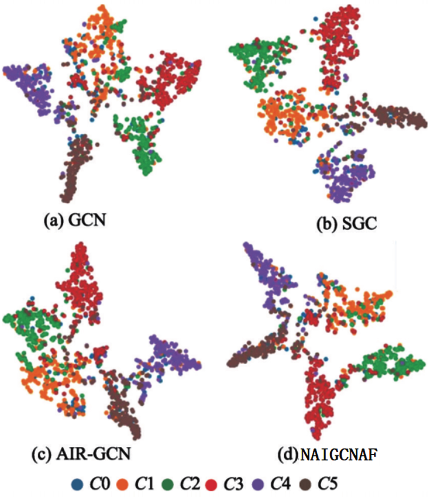
Visualization of Citeseer dataset.

From the Fig. 4, it can be observed that for the Citeseer dataset, the distribution of nodes presented by GCN is relatively chaotic, with clusters of nodes mixed with many different colors. The visualization node distribution of SGC, AIR-GCN, and NAIGCNAF is more reasonable, Compared to SGC, AIR-GCN, and NAIGCNAF, the NAIGCNAF has the best visualization effect, with higher aggregation of nodes within the cluster and clearer boundaries between different clusters. For example, the cluster structures of C1 and C2 in Figure (d) are more compact than the corresponding structures in Figures (b) and (c). Based on the visualization results in Fig. 4 and the average accuracy results in Table 2, it can be seen that the performance of NAIGCNAF is superior to other benchmark algorithms in node classification tasks. Only through visual image display and numerical presentation of node classification results, the actual impact of each improved part on algorithm performance cannot be obtained. We will delve into the practical significance of attention mechanisms and the role of two information constraints.

4.5 Variant analysis of algorithms

Considering the different combinations of consistent regularization loss and differential loss, three variants of the NAIGCNAF algorithm were proposed for ablation experiments to demonstrate the effectiveness of adding consistent regularization loss and differential loss. These four algorithms were run on three datasets, and the average accuracy of 10 random runs was reported. The experimental results are shown in Fig. 5. The four abbreviations in the legend represent: NAIGCNAF-o represents NAIGCNAF without L _c and L _d constraints, NAIGCNAF-d represents NAIGCNAF with only the differential constraint L _d , NAIGCNAF-c represents NAIGCNAF with only the consistent regularization constraint L _c , and NAIGCNAF represents the complete version of NAIGCNAF with both the consistent regularization constraint Lc and the differential constraint L _d .

Analyzing Fig. 5, the following conclusions can be drawn:

On the three datasets, the accuracy of the complete version of NAIGCNAF with both the consistency regularization constraint Lc and the differential constraint Ld is better than the other three variant algorithms. This indicates that using these two constraints simultaneously improves the classification performance of the algorithm.

The classification results of NAIGCNAF-d, NAIGCNAF-c, and NAIGCNAF are superior to NAIGCNAF-o on all datasets, indicating that using both constraints alone or simultaneously can improve the classification performance of the algorithm. These results validate the effectiveness of these two constraints.

Comparing the results in Fig. 5 and Table 2, it can be seen that, compared with the benchmark algorithm AIR-GCN, only the supervised loss term NAIGCNAF-o performs better in classification. This indicates that adding an attention mechanism in the fusion module has a positive impact on the performance of the algorithm. The basic framework proposed in this article is stable and has better performance.

Fig. 5

Node classification results of NAIGCNAF and variants.

4.6 Analysis of attention mechanism

In order to investigate the actual effect of adding attention mechanisms in the fusion module, this section provides a detailed analysis of the learning details of the attention layer. Plot the trend of the average value of attention generated by the attention layer on three datasets, and mark the maximum and minimum values, as shown in Fig. 6. The x-axis represents the number of iterations, and the y-axis represents the average value of attention. In the legend, HirAtt, HaggAtt, MinAtt, and MaxAtt represent the attention value of the neighborhood interaction term, the attention value of the neighborhood aggregation term, the minimum attention value, and the maximum attention value, respectively.

Fig. 6

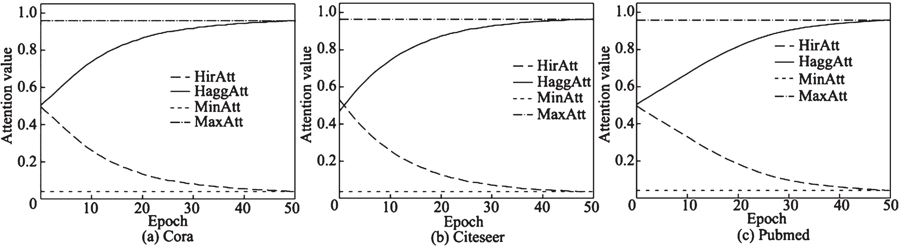
Change of attention value.

The experimental results demonstrate that, at the beginning of training, the average attention values of the neighborhood aggregation terms and neighborhood interaction terms are around 0.5, and they undergo significant changes during the training process. For instance, on the Citeseer dataset, the initial value of the average attention value of the neighborhood interaction term is 0.5. As the algorithm iterates, this value gradually decreases, and the final convergence value approaches 0. On the other hand, the average attention value of the neighborhood aggregation terms continues to increase with training, surpassing 0.9 after 30 iterations. These experimental results indicate that the attention layer in the adaptive fusion module can gradually learn the importance of different embedded representations. Combined with the accuracy results of NAIGCNAF-o in Fig. 5, the effectiveness of the attention mechanism during the learning process of the NAIGCNAF algorithm can be determined.

Analyzing the evolution of attention values during training can provide insights into the learning patterns, interpretability, robustness, and impact on performance of the attention mechanism. By studying these dynamics, we can gain a deeper understanding of how attention influences the neighborhood aggregation and interaction terms and how it contributes to the model’s behavior and performance.

4.7 Convergence analysis

The experiment compared the convergence of NAIGCNAF and the benchmark algorithm AIR-GCN, and plotted the accuracy curves of the two algorithms during training on three datasets. The results are shown in Fig. 7.

Fig. 7

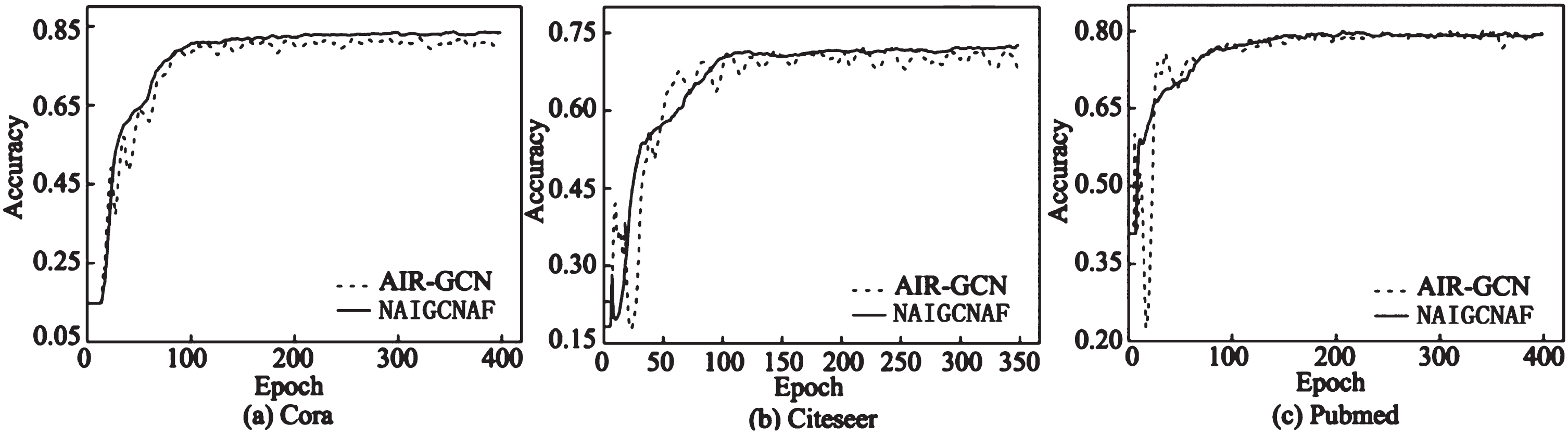
Convergence results.

The results show that the rate of convergence of NAIGCNAF is generally faster than that of the benchmark model AIR-GCN on the three data sets, and the accuracy distribution of the training process is more stable. Therefore, NAIGCNAF algorithm shows faster rate of convergence and higher convergence stability.

Analyze the impact of the dimension p of the attention layer, the consistency regularization loss weight t, and the difference loss weight r on the algorithm’s node classification performance through experiments. Each time one analysis parameter is determined, two non analysis parameters are fixed, and the numerical value of the analysis parameter is changed to study its impact on the algorithm.

The attention layer dimension p is a hyperparameter that can adjust the model structure. Considering the computational complexity of the algorithm, the attention layer dimension p is taken as 15 integer values in the interval [1, 15]. Keeping other parameters unchanged, run the algorithm 10 times on each of the three datasets and report their average accuracy values, as shown in Fig. 8.

Fig. 8

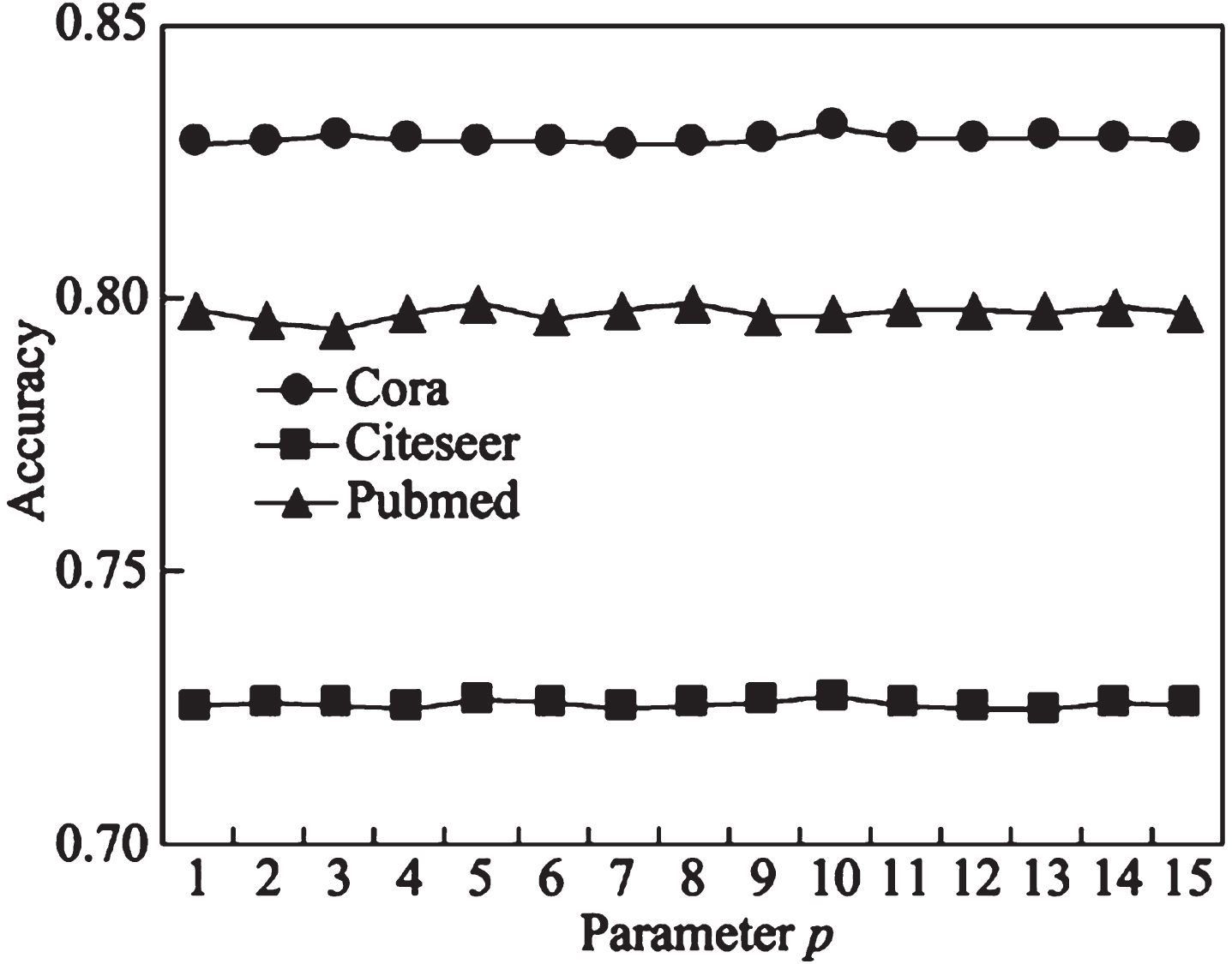
Influence of parameter p.

The experimental results show that: (1) the fluctuation amplitude of the three broken lines is relatively small, indicating that within the above value range, the p-value has little impact on the accuracy of the performance index standard, indicating that the sensitivity of the algorithm in this paper to parameter p is low. (2) On the Cora, Citeseer, and Pubmed datasets, the algorithm has the highest classification accuracy when the dimension p of the attention layer is set to 10, 8, and 10, respectively. (3) Based on the experimental results in Fig. 8 and Table 2, even in the worst case of classification performance, NAIGCNAF performs better compared to other benchmark algorithms.

Figure 9 shows the impact of consistency regularization loss weight t on the classification performance of algorithm nodes, and its value was adjusted from 10^-4 to 1.0 in the experiment. It can be observed that on all three datasets, as the weight t increases, the classification performance of the algorithm slowly improves. When t is within the range of 10^-4 to 1.0, the classification performance of NAIGCNAF is stable, indicating that the sensitivity of NAIGCNAF to parameter t is relatively low. When the consistency regularization loss weight t is set to 1.0 on three datasets, the algorithm has the highest classification accuracy.

Fig. 9

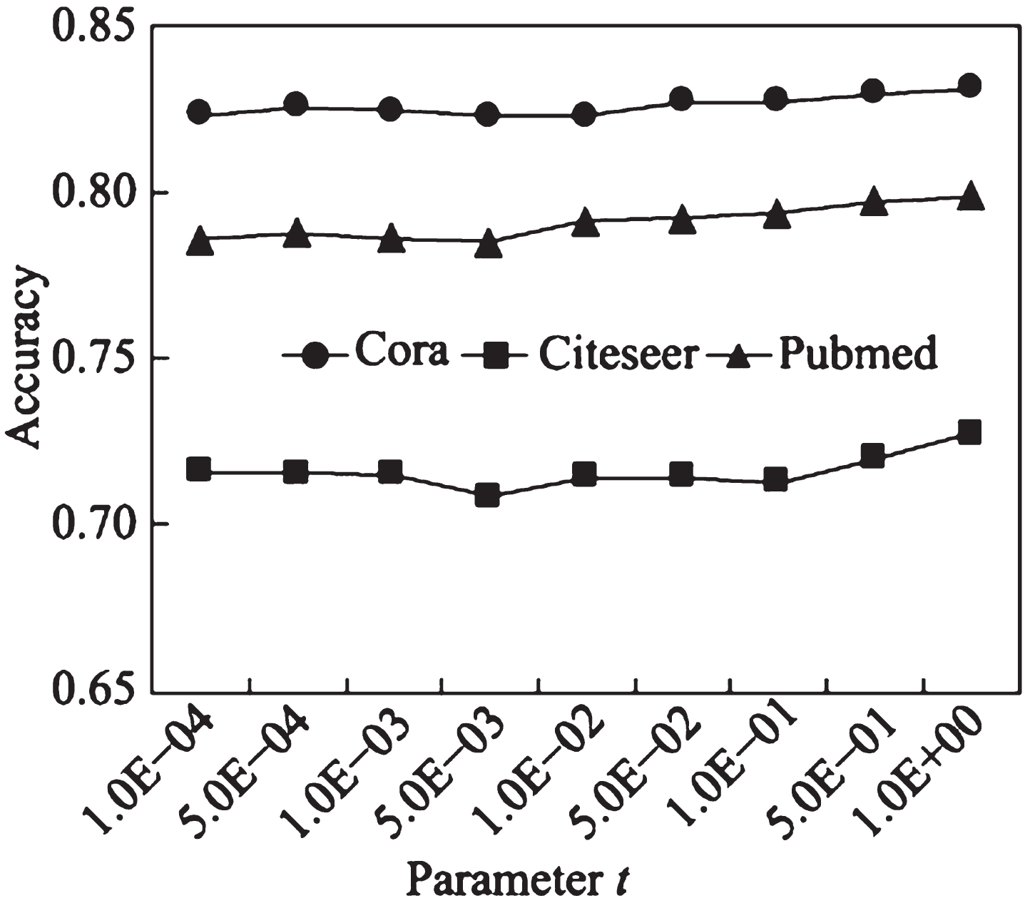
Influence of parameter t.

Figure 10 shows the impact of differential loss weight r on the classification performance of algorithm nodes, and its value was adjusted from 10^-5 to 10^-1 in the experiment. In Fig. 10, it can be observed that on three datasets, the accuracy of NAIGCNAF shows an unstable state when r is within the range of 10^-5 to 10^-1, indicating that the algorithm has a high sensitivity to parameter r. On three datasets, the algorithm has the highest classification accuracy when the differential loss weight r is set to 10^-4.

Fig. 10

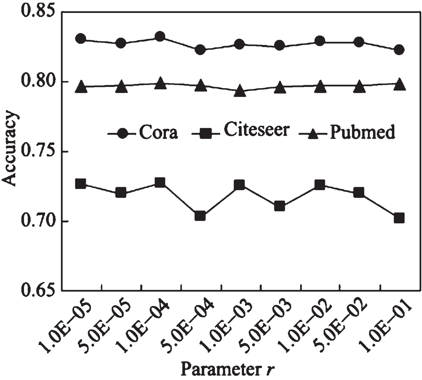
Influence of parameter r.

Analyzing the specific properties of the NAIGCNAF algorithm that contribute to its faster convergence can provide valuable insights into its effectiveness and efficiency. Understanding these properties can help to identify the strengths and limitations of the algorithm and make informed decisions regarding its implementation.

When discussing the faster convergence of the NAIGCNAF algorithm, several properties can be considered:

-Adaptive Feature Aggregation: The NAIGCNAF algorithm utilizes an adaptive feature aggregation mechanism that dynamically adjusts the importance of each feature during the aggregation process. This adaptive mechanism allows the algorithm to focus on the most informative features and discard less relevant ones. By doing so, the algorithm can converge faster by leveraging the most discriminative information from the input data.

-Attention Mechanism: The attention mechanism in NAIGCNAF plays a crucial role in determining the relevance and importance of each neighborhood interaction term. By assigning attention weights, the algorithm can selectively emphasize or downplay certain neighborhood interactions, based on their importance. This attention mechanism helps the algorithm to focus on the most influential interactions, leading to faster convergence by prioritizing the most relevant information.

-Neighborhood Interaction Learning: NAIGCNAF incorporates a neighborhood interaction learning component, which models the pairwise relationships between nodes in the graph. By learning these interactions explicitly, the algorithm can capture more nuanced dependencies and patterns in the data. This enhanced modeling of neighborhood interactions contributes to faster convergence by incorporating more comprehensive contextual information.

-Regularization Techniques: NAIGCNAF may use regularization techniques such as dropout or weight decay to prevent overfitting and improve generalization. These regularization techniques can contribute to faster convergence by reducing the impact of noisy or irrelevant features, leading to a more efficient learning process.

While the NAIGCNAF algorithm offers faster convergence, it is essential to consider potential trade-offs:

-Computational Complexity: The adaptive feature aggregation and attention mechanisms in NAIGCNAF introduce additional computational complexity compared to traditional GCN algorithms. This increased complexity may require more computational resources and time for training and inference.

-Interpretability: While NAIGCNAF ‘s adaptive feature aggregation and attention mechanisms contribute to faster convergence, they may make the model less interpretable. The complex interactions and weights assigned by these mechanisms can be challenging to interpret and understand, limiting the explainability of the algorithm.

-Sensitivity to Hyperparameters: The performance and convergence speed of NAIGCNAF can be sensitive to the choice of hyperparameters. Tuning these hyperparameters effectively may require additional effort and experimentation.

4.8 Complexity analysis

First, analyze the time consumption of each module of the algorithm to obtain the overall time complexity, and then call the torchsummary tool to estimate the cache size occupied by the model and calculate its space consumption. Assuming n is the total number of nodes, m is the total number of edges, d is the attribute dimension, d _i represents the feature dimension output by the i-th graph convolutional layer, and d’ represents the dimension of the attention layer.

For the GCN algorithm, the calculated Time complexity is O(md_1  + ndd_1  + md_2  + nd₁d₂). ndd₁ and nd₁d₂ involve the multiplication of feature representation and parameter matrix, while md₁ and md₂ represent the time consumption of neighborhood aggregation process. The total number of parameters on the Cora, Citeseer, and Pubmed datasets is 0.09 MB, 0.23 MB, and 0.03 MB, respectively. The Time complexity of AIR-GCN is O(md_1  + ndd_1  + md_2  + nd₁d_2  + nd₁). It adds element multiplication and addition to the calculation of neighborhood interaction terms, and the resulting time cost is about O(nd₁). AIR-GCN adopts a dual channel graph convolutional structure, so its space consumption is approximately twice that of the GCN algorithm. The total number of parameters on the Cora, Citeseer, and Pubmed datasets is 0.18 MB, 0.45 MB, and 0.06 MB, respectively. The overall Time complexity of NAIGCNAF is O(md_1  + ndd_1  + md_2  + nd₁d_2  + nd_1  + nd₁d^′). Compared to the benchmark algorithm AIR-GCN, NAIGCNAF adds an attention layer in the fusion module to inject label information into the fusion process, with a time consumption of approximately O(nd₁d’). Due to the usual limitation of d’ being smaller than d₁ to obtain dense attention value intermediate vectors, NAIGCNAF and AIR-GCN have similar computational time costs. The total number of parameters on the Cora, Citeseer, and Pubmed datasets is 0.18 MB, 0.45 MB, and 0.06 MB, respectively. Therefore, NAIGCNAF and AIR-GCN have similar space consumption. The detailed content is shown in Table 3.

Table 3

Algorithm parameters and complexity

Data set	Parameter quantity/MB
	GCN	AIR-GCN	NAIGCNAF
Cora	0.09	0.18	0.18
Citeseer	0.23	0.45	0.45
Pubmed	0.03	0.06	0.06
Complexity(O)	md1 + ndd1 +	md1 + ndd1 +	md1 + ndd1 +
	md2 + nd1d2	md2 + nd1d2	md2 + nd1d2 +
		+ nd1	nd1 + nd1d′

When discussing the complexity of the proposed method, it is useful to compare it with existing benchmark algorithms. This allows researchers and practitioners to understand the computational requirements and potential scalability of the proposed method. Here are a few points to consider:

-Time Complexity: Analyzing the time complexity of the proposed method in comparison to benchmark algorithms can provide insights into its efficiency. For example, if the proposed method has a lower time complexity, it can process larger datasets or perform more extensive computations within a reasonable time frame.

-Space Complexity: Understanding the space complexity of the proposed method is crucial, as it indicates the amount of memory required for its execution. Comparing the space complexity with benchmark algorithms can help assess the feasibility of running the proposed method on different hardware configurations and limitations.

-Empirical Comparisons: Conducting empirical comparisons between the proposed method and benchmark algorithms on various datasets can provide a comprehensive understanding of their relative performance. Evaluating factors such as accuracy, convergence speed, and resource utilization can help determine the practicality and feasibility of the proposed method in real-world scenarios.

-Scalability: Assessing the scalability of the proposed method is essential to understand its feasibility in handling larger datasets or more complex tasks. If the proposed method demonstrates good scalability compared to benchmark algorithms, it can be considered a promising solution for practical applications.

4.9 Discuss

-Performance of Previous Methods:

Traditional Graph Convolutional Networks (GCNs) suffer from limitations such as limited receptive field, over-smoothing, and difficulty in capturing long-range dependencies. These limitations can result in suboptimal performance and hinder their effectiveness in tasks requiring a comprehensive understanding of the graph structure and complex relationships.

-Limitations of Previous Methods:

a) Limited Receptive Field: Previous methods often struggle to capture information from distant nodes in the graph. This limited receptive field restricts their ability to model long-range dependencies and capture global graph patterns effectively.

b) Over-smoothing: As GCNs propagate information across the graph, the representations of nodes tend to become overly similar, leading to over-smoothing. Over-smoothing can cause a loss of discriminative power and hinder the ability to distinguish between different nodes in the graph.

c) Difficulty in Capturing Long-Range Dependencies: Capturing long-range dependencies is challenging for previous methods, as they rely on a fixed number of graph convolutional layers with local aggregation. This limitation hampers their ability to understand complex relationships that span across distant nodes in the graph.

-Overcoming Limitations with NAIGCNAF:

NAIGCNAF addresses the limitations of previous methods and seeks to overcome them by introducing several key features:

a) Adaptive Fusion Module: The adaptive fusion module in NAIGCNAF incorporates an attention mechanism that allows nodes to selectively aggregate information from neighboring nodes. This attention mechanism enables the model to focus on relevant nodes and capture long-range dependencies effectively, overcoming the limited receptive field issue.

b) Label-guided Attention: NAIGCNAF leverages label information to guide the attention mechanism. By incorporating label information, NAIGCNAF can assign higher attention to nodes that are more relevant to the target task and suppress the influence of less informative nodes. This improves the model’s ability to capture task-specific information and enhances its performance.

c) Adaptive Information Refinement: NAIGCNAF dynamically refines node representations by adaptively aggregating information from neighboring nodes. This mechanism helps overcome over-smoothing issues by allowing nodes to refine their representations based on the importance and relevance of neighboring nodes, preserving their discriminative power.

By incorporating these features, NAIGCNAF aims to improve the performance of traditional GCNs and overcome their limitations in capturing long-range dependencies, limited receptive field, and over-smoothing issues. It provides a more comprehensive understanding of the graph structure and complex relationships, leading to enhanced performance in various graph-based tasks.

5 Conclusion and outlook

The contributions of the paper include the development of the NAIGCNAF model, which combines neighborhood aggregation and neighborhood interaction to enhance graph representation learning. The model incorporates an attention mechanism that adaptively learns fusion weights, improving the information extraction process. Additionally, the inclusion of consistency regularization and difference constraints further enhances the quality of the learned representations.

The research results demonstrate the effectiveness of the NAIGCNAF model on various downstream tasks such as node classification and link prediction. The model outperforms existing graph representation learning methods, achieving higher accuracy and better performance. The attention mechanism enables the model to adaptively fuse information, capturing the most relevant features for each node. The consistency regularization and difference constraints improve the consistency of node features and the distinction between embedded representations, respectively.

However, the paper does not explicitly mention limitations or potential directions for future research. It would be beneficial for future studies to explore the scalability of the proposed model to larger graphs and evaluate its performance on more diverse and complex datasets. Additionally, investigating the interpretability of the learned representations and exploring techniques to reduce computational complexity could be potential directions for future research.

The performance of NAIGCNAF surpasses that of benchmark neural network models in downstream tasks. However, future research aims to improve the model’s efficiency, making it suitable for larger networks. Furthermore, there is a need to expand the model’s depth to obtain more depth information. Consequently, this will improve the model’s performance, making it more effective in solving complex graph representation problems.