Sage Journals: Discover world-class research

Abstract

Load balancing is an element that must exist for a cloud server to function properly. Without it, there would be substantial lag and the server won’t be able to operate as intended. In a Cloud computing (CC) establishing, load balancing is the process of dividing workloads and computer resources. The distribution of assets from a data centre involves many different factors, including load balancing of workloads in cloud environment. To make best use each virtual machine’s (VM) capabilities, load balancing needs to be done in a way that ensures that all VMs have balanced loads. Both overloading and underloading are examples of load unbalance, and both of these types of load unbalance could be fixed by using techniques created especially for load balancing. The research that has been done on the subject have not attempted to take into account the factors that affect the problem of load unbalancing. Results indicate that the LSTM and DForest-based load balancing approach significantly improves cloud resource utilization, reduces response times, and minimizes the occurrence of overloading or underloading scenarios. To effectively design those programmes, it is essential to first understand the advantages and disadvantages of current methodologies before developing efficient AI-based load balancing programmes. Compared to existing method the proposed method is high accuracy 0.98, KNN accuracy is 0.97, SVM accuracy is 0.99, and DForest accuracy is 0.987.

Keywords

Load balancing artificial intelligence machine learning DForest Long Short-Term Memory

1 Introduction

In the past few years, cloud computing has become increasingly significant for numerous enterprises. As a notion of immediately shared resources through heavily internet-based apps, cloud computing originally served to meet user needs for commodity processing availability or to allow users to buy services from the cloud as needed [1]. Technology used in virtualization is a crucial part of cloud computing. Utilising virtualization technology, several computing nodes are linked to a single resource pool. Using the Internet, users can use the resource pool’s resources on a “pay as you go” basis [2 –4], and the resource may be dynamically changed to meet the demands of the users. Cloud computing services may be shared by thousands of users, significantly lowering the economic cost for users. Customers and cloud service providers may both profit from virtualization technologies dynamic resource scheduling approaches. Task planning has become a major concern due to the constant increase in workload at cloud data centres, which could eventually result in a shortage of cloud assets. Effective resource scheduling not only completes tasks in the shortest amount of time, but also increases the resource utilisation ratio, i.e., decreases the use of resources. Because of this, cloud computing is still in its infancy and requires more study to appropriately map tasks to cloud resources and achieve the scheduling objective (improving the quality-of-service characteristics).

Cloud task scheduling is the act of establishing beginning of each activity in a process while taking into account the workflow’s dependencies and task expiry periods for separate jobs, the task scheduling methods is typically straightforward. However, interdependence of jobs of a process might make its scheduling a tough challenge [5]. Following scheduling and prioritization of tasks, appropriate resources should be assigned to them. Each job necessitates a certain processing resource based on its execution time [8, 9]. Inadequate resource provisioning not only increases workflow execution time, cost, and energy consumption, but also reduces resource use efficiency. On the other side, disregarding resource load balancing can drastically reduce resource efficiency. In resource allocation is the process of assigning available resources to the desired cloud apps through the internet [8, 9]. If the resource allocation is not handled accurately, it deprives services. Resource provisioning address this issue by allowing service providers to control resources for each individual module [14]. When the earliest dispersed computer systems went into place, the idea of “load balancing” already existed. In order to maximise productivity, reduce response times, and boost resilience to failures by avoiding overloading the systems, it means precisely what the name implies: equally spread the workload among a number of computers [10]. The topic of load balancing in cloud data centres is currently a popular topic. When deploying activities, it is essential to select the ideal physical host quickly in order to perform load balancing across cloud data centres [11]. The effective use of resources is dependent on task scheduling and load balancing techniques to prevent the arbitrary allocation of sources. Load balancing and task scheduling are significant actors in the CC environment [12].

Task scheduling, VM allocation, and resource allocation are critical for effective and efficient workload management that minimize response time while simultaneously ensuring service level agreement (SLA) [13, 14]. Reducing SLA violation and response time throughout the job scheduling was not adequately handled by conventional algorithm. To address these issues, a task scheduling-based load balancing approach called leveraging the power of Long Short-Term Memory (LSTM) and hybrid machine learning, load balancing in cloud computing can be optimized to enhance performance and resource allocation.

Load balancing is a fundamental element for the efficient functioning of cloud servers, ensuring minimal latency and optimal resource utilization. In the context of CC, load balancing involves the intelligent distribution of workloads and computer resources across servers to maintain equilibrium and meet application demands. Effective load balancing is vital for maximizing the capabilities of each virtual machine (VM) and avoiding scenarios of overloading or underloading, which can lead to performance bottlenecks.

However, despite its significance, load balancing in cloud environments remains a challenging task due to the dynamic and unpredictable nature of workloads. Traditional load balancing approaches often struggle to adapt to fluctuating demands, resulting in inefficient resource allocation and degraded system performance.

This research proposes a novel task scheduling-based load balancing approach that harnesses the power of LSTM and hybrid machine learning techniques to optimize load balancing in cloud computing. LSTM, known for its ability to capture temporal dependencies in data, is utilized to predict future workload patterns accurately. When combined with a hybrid machine learning strategy, including techniques like DForest, the approach empowers cloud systems to make real-time load balancing decisions efficiently.

By integrating LSTM and hybrid machine learning, cloud resource utilization can be significantly improved, response times reduced, and the occurrence of load imbalances minimized. This approach offers a powerful solution to enhance cloud server performance and resource allocation, contributing to improved service delivery and increased user satisfaction.

In this paper, we present the results of comprehensive experiments that demonstrate the effectiveness of the LSTM and DForest-based load balancing approach. The study showcases its ability to outperform traditional methods and highlights the advantages it offers in terms of dynamic adaptability to varying workload scenarios.

To effectively design and develop AI-based load balancing programs, a thorough understanding of the advantages and disadvantages of existing methodologies is paramount. By identifying the limitations and exploring the full potential of the proposed approach, cloud service providers can lay the groundwork for more efficient and intelligent load balancing in their infrastructures.

The Priority-based Modification Hierarchical Earliest Finish Time (PMHEFT) solution is going to be less complicated and economical effective in distributing load across network infrastructure (cloud computing). Our suggested method balances loads both dynamically and statically [15]. The workload in a cloud computing system refers to the distribution of various workloads across VMs. The workload rebalancing issue can be defined in a number of methods, as shown below. Task distribution means randomly assigning of just a handful of tasks to various Physical Machines (PMs), which then distribute those jobs to various Virtual Machines (VMs) of corresponding PM [16]. Huge VMs have a connection in CC by preemption and non-preemptive resource distribution, nevertheless supplies aren’t allocated uniformly and just a handful of VMs have the capacity to complete the tasks. When a job is supplied in the public internet, all VMs must work in asynchronous fashion and must do the task swiftly and simply [17].

This article introduces a novel machine learning-based AI solution that thoroughly analyses numerous load balancing algorithms available on the market. The primary purpose of designing this proposed algorithm is to address the challenges posed by load unbalancing in cloud data centres. The novelty of our approach lies in its focus on understanding and mitigating factors leading to load unbalancing. By ensuring balanced loads on each VM, we aim to maximize the utilization of VM capabilities and optimize resource allocation. To develop efficient AI-based load balancing programs, it is crucial to comprehend the advantages and disadvantages of existing methodologies. Therefore, our research explores various load balancing techniques and provides a comprehensive evaluation, laying the foundation for designing an effective AI-based solution.

1.1 Key contribution

This analysis serves as a basis for designing the efficient AI-based load balancing program.

The machine learning-based AI solution ensures balanced loads on each VM, leading to optimal utilization of VM capabilities. By avoiding overloading and underloading, the proposed method enhances resource efficiency and minimizes resource wastage.

The proposed AI-based load balancing program exhibits high scalability and adaptability, making it suitable for various cloud environments and workload patterns. This adaptability enables it to handle varying demands and maintain performance under dynamic conditions.

Leveraging machine learning techniques, the AI-based solution facilitates real-time decision making for resource allocation. The system can quickly respond to changes in workload demand, ensuring efficient load distribution and minimizing response times.

The AI-driven load balancing approach demonstrates versatility and generalizability, making it applicable not only to cloud computing but also to resource allocation challenges in other domains and distributed systems.

1.2 Limitations of the study

Limited Dataset: The effectiveness and generalizability of the proposed AI-based load balancing program heavily rely on the size and diversity of the dataset used for training and evaluation. A limited dataset may restrict the model’s ability to handle all potential workload scenarios.

Experiment Protocol: The article may lack a detailed explanation of the experiment protocol used for evaluating the proposed AI-based load balancing approach. A comprehensive experiment protocol is essential to ensure the reproducibility and comparability of the results.

Model Complexity: While the article highlights the high accuracy of the proposed method, it might not delve into the complexity of the AI model itself. A more in-depth analysis of the model’s complexity could provide insights into its computational overhead and feasibility in practical cloud environments.

Limited Practical Implications: Although the article discusses the managerial significance and potential applications of the proposed AI-based load balancing program, the practical implications in real-world cloud settings might require further exploration and validation.

2 Related works

There are several research ideas and initiatives relating to high-performance computing and cloud-based computing that are currently in various phases of development. These ideas and initiatives are being developed by a variety of organisations.

Karimzadeh Parizi et al. [18] proposed Woodpecker Mating technique (WMA), a novel search technique with natural inspiration, is used to tackle difficult architectural optimization issues. A based on populations metaheuristic method called the WMA imitates woodpeckers’ mating habits. The force of the pounding sound served as inspiration. The woodpecker populations in WMA is split between males and females. According to the volume generated by their drum sound, the female woodpeckers approached the male woodpeckers. The WMA method along with other metaheuristic algorithms were compared in terms of performance using 19 benchmarking operates, spanning unimodal in nature multimodal in nature, and blended functions. Furthermore, employing 13 highly complex multidimensional and unicameral benchmarks functions, the performance of WMA is compared to that of 8 of the top meta-heuristic systems.

Karimzadeh Parizi et al. [19] proposed opposition-based acquiring knowledge, a newly improved variant of the Woodpecker Mating Algorithm (WMA) called the OWMA seeks to build both exploring and exploiting capabilities and achieve a concurrent equilibrium among these two stages. The new Distance Opposition-based Learning (DOBL) process, which enhances exploration, variety, and integration, is the initial of three key processes that make up this enhancement. The second mechanism is the distribution of the local recollection of searching agents’ particular experiences for increasing their productive potential. The second method involves using a self-regulating and dynamical strategy to modify the H parameter in order to enhance the performance of the Running Away function (RA). A number of the newest and popular metaheuristic algorithms studied in the study literature were compared to the suggested algorithm’s capacity for solving 23 benchmarks functions of mathematics. On five healthcare samples and three approximate function datasets, the suggested method is also employed as a Multi-Layer Perceptron (MLP) neural network trainer to address the labelling issue.

Morteza Karimzadeh Parizi et al. [20] proposed the sine cosine algorithm (SCA) with a woodpecker mating algorithm (WMA) were combined to create HSCWMA, an innovative metaheuristic algorithm for addressing challenges in optimization. Notwithstanding the WMA algorithm’s significant potential for discovery, utilization requires to be increased, particularly throughout the first few iterations. Additionally, SCA makes the most of both the cosine as well as sine connections, but it lacks an adequate mechanism for implementing successful explorations. The female woodpeckers in WMA are updated in HSCWMA using the SCA by Levy flying mechanism’s enhanced mathematical search procedures. Additionally, the combination of techniques that is suggested uses the current searching storage for every search element. In order to build both exploration and exploitation qualification and provide an evolving equilibrium across these two stages, the HSCWMA is being proposed. It will make advantage of the investigation capabilities of the WMA with Levy flight, as well as the mining susceptibilities of the SCA including the local search storage. The suggested approach is examined for performance using 28 reference functions in mathematics. When evaluated against a number of some of the most modern and well-liked metaheuristic algorithms, the HSCWMA method surpasses them for resolving nonconvex, indivisible, and extremely challenging optimization queries.

Karimzadeh Parizi et al. [18] proposed In an effort to address the ED issue while taking into account nonlinear features of power plants, which include valve point effects (VPE), restricted operational zones (POZ), ramp rate restrictions, various fuel alternatives, and transport loss, the Woodpecker Mating Algorithm (WMA) is utilized. The WMA method is a revolutionary metaheuristic algorithm that was motivated by the level of sound (a physical property) and avian woodpeckers’ reproductive habits. Several test systems with various operation parameters and features are used for the implementation of WMA in order to demonstrate its effectiveness in resolving the ED problems. The outcomes are contrasted against the most recent and effective techniques described in the available research. The simulation findings are encouraging and provide the best fuel cost of manufacturing, demonstrating the effectiveness of the WMA to address the ED challenge.

Jiali Zhang et al. [21] proposed the HWMWOA combines the WMA with the Whale Optimization Algorithm (WOA). WOA is an algorithm of great power without the benefit of being able to perform searches globally using few control parameters. However, WOA is more inclined to become stuck in regional optimum indications, miss out on demographic variety, and experience early converging. The HWMWOA algorithm’s primary objective was to eliminate WOA’s shortcomings. Several basic mechanisms make up this improvement. Initially an amended version of the WMA’s position updating calculation based on effective investigation is incorporated into the HWMWOA. Secondly, the suggested hybrid approach is given a new self-regulating Cauchy mutations activator. The proposed HWMWOA method uses arithmetic to generate spiral movements with a new search guide pattern as a final step.

Gong et al. [22] proposed on the graphics processing unit (GPU) may accelerate WMA to solve optimization issues in simultaneously increasing accelerate and reducing WMA time to execution while maintaining the accuracy of the best possible outcomes. The suggested approach offers numerous methods for creating numbers that are random on the host system, bulk transferring those numbers to the GPU, initializing and monitoring the first set of numbers while concurrently on the GPU, and refreshing and assessing the positions of the seeking agencies. To choose the most effective drug, it likewise employs a diminishing method. The comparisons between the concurrent and serial WMA depend on the CEC2017 test features and a traditional benchmarking. In order to indicate each quickness of the GWMA, additional simultaneous MAs evaluate the GWMA’s time of operation.

In comparison with the static methods, dynamic algorithms [23] can adjust their behaviour in accordance with the dynamic nature of the CC system. This contrasts with static methods, which cannot change. DLBA offers improved fault performance and tolerance, even though it is challenging to implement. This behaviour might help compensate for some of the drawbacks of the passive strategy, but that approach might have some drawbacks to begin with. These policies are referred to as section policies, information policies, transfer policies, and placement policies, respectively, throughout this document. The way responsibilities are carried out can then be categorised on the basis of these policies, which serve as the cornerstone.

Shahdi-Pashaki et al. [24] came up with the idea for the Genetic Algorithm, which is a self-replicating piece of predictive software. An examination of Darwin hypothesis of evolution serves as the foundation for this work. Genetic algorithms (GA) are the high-performance method of choice when it comes to discovering solutions to difficult optimization problems. In contrast to earlier models, this one considered a realistic multi-service dynamic scenario in which customer locations could shift at different times and where server cluster handled only a single type multimedia activity for the purpose of optimising performance in two different ways at the same time. In this scenario, customer locations could shift at different times, and respectively server cluster handled only a single type of multimedia activity. This was done so that we could simultaneously achieve both of our performance objectives to their fullest potential.

Renggli et al. [25] concentrate on more-performance machine learning strategies, have their primary emphasis on rapidly expanding corporate data as the audience for whom they are aiming their work. This technique of design shows promises in addressing the communication bottlenecks of parallel and distributed processing when it is applied to the ever-evolving data requirements of businesses to power machine learning. The goal of this application is to make businesses more efficient. This is a precondition for the successful implementation of machine learning.

Recovery time goals (RTOs), and recovery point objectives, also referred to as RPOs, are two concepts that Andrade, E., & Nogueira, B. [26] have placed a significant amount of significance on RTO. The authors place a strong emphasis on the reality that average cost of downtime for information technology is $5,600 per minute. Fortunately, most companies will never have to deal with a scenario in which they are held up for more than a few hours. This kind of situation can be extremely detrimental to a company bottom line and lead to substantial financial losses. The authors claim that the new database-based recovery strategy reduces the amount of time it takes to re-establish a system following a failure to just 4.5 seconds by utilising the most cutting-edge technological models. This would be a significant improvement over the previous approach.

Cloud service providers (CSPs) building data centres by high-speed computing capabilities suit expectations cloud clients. Finding an optimum schedule in an NP-hard problem is never simple. A approach for suggested resource-aware dynamic scheduling of tasks put into practise by Nabi [27]. In terms of ARUR, throughput, and makespan, the Resource Aware Dynamic Load Balancing Algorithm (DRALBA) approach demonstrated significant improvements. Three well-known datasets, including HCSP, GoCJ, and Synthetic workload, were used in the simulation experiments, which were carried out using the simulation application Cloudsim. In terms of average resource utilisation (ARUR), makespan, throughput, and average response time (ART), the results of the proposed technique are then contrasted with those of the RALBA, Dynamic MaxMin, DLBA, and PSSELB scheduling algorithms.

With regard of the pay-as-you-go system for dynamically allocating computer resources to client’s usage, cloud computing recently made progress. Ibrahim [28] suggests looking at the goals of recent, state-of-the-art scheduling algorithms in order to map HPC activities to resources. The empirical investigation shows that it is not enough to schedule independent jobs on machines centred only on execution time, throughput, and the average resource utilisation ratio; machine-level load balancing needs to be considered as well to make sure that the computing capacity in a cloud system is fully utilised. The resource-aware load balancing algorithm (RALBA) heuristic fared better than the rivals and appears to offer the greatest performance/complexity ratio for resource utilisation and machine-level load balancing.

3 Problem statement

A crucial problem in cloud computing is load balancing determines efficiency of system. The challenge is attain optimal resource utilization, reduce response time, and prevent overload of any particular server. Traditional load balancing techniques have limitations in adapting to changing workloads and fail to provide accurate predictions of resource demands. Consequently, it is necessary to develop an intelligent load balancing system that can dynamically allocate resources and improve overall performance of cloud system. This can be achieved through the integration of hybrid machine learning techniques, which can provide more accurate predictions of workload demands and help to optimize resource allocation in real-time [29]. For example, imagine a scenario where a server without load balancing is serving a high-traffic website. Without load balancing, all incoming requests are directed to a single server, overwhelming its resources and causing latency issues. As a result, users may experience slow page loading times, timeouts, or even server crashes. However, by implementing load balancing techniques, such as distributing incoming requests across multiple servers, the system can handle the traffic efficiently, ensuring smoother user experiences and minimizing the risk of significant lag [30].

4 Proposed method

The proposed method includes three phases: task assignment, LSTM auto encoder, and load balancing to give tangible and optimum solution to problem resource management in cloud environment. These three stages collaborate by interacting one another. In first phase requests {request₁, request₂, . . . . , request_N} provided by {User₁, User₂ . . . . . , User_N} are broken into subunits called tasks {T₁, T₂ . . . . , T_X}, which are allocated to computing instances’ called {VM₁, VM₂ . . . . , VM_Y} for execution. The assignment is accepted and performed on the selected VM by the cloud computing platform if doing so is not inconsistent with the service level agreement (SLA). The cloud computing platform won’t carry out the work unless the VM’s load increases and the VMs’ load balancing status changes. During the second phase, VMs loaded with the user’s job execute the task while also forecasting resources use for the following interval. Filled blocks represent allotted VMs, whilst empty blocks represent de/unallocated VMs. Depending on its setup, each cloud server has its own load analyzer, which collect each VM’s expected resource consumption statistics and identifies the occurrence of normal/busy ahead of time. If the expected resources utilization exceeds the server’s resource capacity, overload is recognized and the necessary activities to reduce its effect are conducted in the third phase. Machine learning algorithms such as RF, SVM, and Dforest algorithm can be employed to tackle issues related to regression and classification, providing effective solutions to these problems.

Load management is performed in the third step by conducting VM assignment and migration to optimize source usage effectively management normal/busy severs. API Unit and AI unit load analyser regularly tells the cluster management about the predicted load at each server employing multifaceted VM placement, that is subsequently used during VM allocation on the chosen server. The methods employ an LSTM auto encoder-based workload predicted to determine if the workload is regular or busy. Is used to make necessary VM migration and balance the cluster’s overall burden. To save power usage, all ideal severs are turned off. The following section provide a full description of each step.

4.1 Task assignment

User first submits user request model requests. Second, the consumer’s request model provides task input to the LSTM autoencoder. User make request cloud computing platform, which processes them, and these needs comprise job flow (i.e., job₁, job₂, . . . . , job_n). A job is made up of numerous tasks, which are represented as job_n ={ T_n,1, T_n,2, . . . . , T_n,m } where T denotes task and m is number of tasks in job. Tasks are non-pre-emptive and independent one another. Given identical condition, task with long task length takes longer to complete than a work with a short task length. Third, the LSTM autoencoder is utilized to choose an appropriate VM for job. Fourth determine if task violates the SLA (deadline) while being processed on selected VM; The job is refused if the SLA is broken; otherwise, it is sent to the chosen VM for handling. Arrival time for the task time_arv is time when task arrives at cloud computing platform, and Dl job’s deadline [31]. For cloud computing system to send messages, work must be finished before the deadline. Ee is the task’s estimated execution time on the specified VM. If the agreement is not broken, the SLA requires time_arv + Ee ≤ Dl; otherwise, a task execution refused. The deadline in this document is as follows: $Dl = tim e_{arv} + Tl / spee d_{slowest}$ (1)

Where Tl is the task length, and speed_slowest is execution speed of slowest VM. Fifth, if the job is rejected, give the LSTM autoencoder a load balancing goal of having all VMs have the same load; otherwise, provide user request result to user. Sixth, once VM completes the work, All VM load situations are delivered to the load balancing model by the cloud computing platform model. Finally, the load balancing model states that the goal is to equalise the load across all VMs. Value to LSTM auto encoder based on VM load.

4.1.1 Load balancing

By guaranteeing the best use of the assets at hand, an efficient load balancing approach is required to maximise the performance of tasks reaction times and eliminate the problem of load balancing between all VMs. Many academics have discussed load balancing techniques in heterogeneous and homogeneous settings, including static load balancing and dynamic load balancing. The main objective of the load balancing approach is to increase the run length of operations by more effectively employing the resources that are accessible, since their abilities for work vary erratically during the course of operations. Low fluctuations in load in VMs will allow static load balancing solutions to focus effectively. while a result, static load balancing mechanism will not function effectively since loads change unexpectedly while the programme runs. In situations when loads fluctuate in real time and servicing needs must be taken into account, dynamic load balancing preferable to static load balancing. The dynamic approaches are extremely important and successful in balancing load among diverse resources due to the network’s quick expansion and need for resources throughout run time [32].

The cloud computing platform receives job that meets SLA and executes it on the designated VM. After completing tasks, each VM has a cumulative; the goal of load balancing is to have all VMs have same burden.

Based on load balancing condition of VMs, the load balancing model provides a goal of load balancing is to equalise the load across all VMs. value to the LSTM autoencoder. Equation (2) define the load of VM_i and the average load of all VMs, respectively: ${load}_{r} = \sum_{q}^{k} \frac{l_{q}}{spee d_{r}}$ (2) ${load}_{avg} = \frac{\sum_{r = 1}^{p} loa d_{r}}{p}$ (3)

Where l_q is length of qth task allocated on VM_r, speed_r is processing speed of VM_r and k is total number of tasks allocated on VM_r.

4.2 Categorization of data types for k-nearest neighbor (KNN) algorithm

According to the K-Nearest Neighbors (K-NN) algorithm, a new instance or collection of data should be categorised under the category that is most comparable to the ones that are already in use. This may sound counterintuitive at first but bear with me. K-Nearest Neighbors is a non-parametric procedure, which means that it does not use parameters and therefore does not make any assumptions about the data that it is analysing. This algorithm does not immediately make use of the training set, it is sometimes referred to as a lazy learning algorithm. This is because it does not use training set. Instead, it will retain the dataset, and the only time it will be used is when it comes time to classify the information. The research make use of SKLEARN and the features that were collected while the data was being processed so that the research can train this KNN model.

4.3 Information storage in long short-term memory (LSTM) networks

Information can temporarily stored in the recurrent neuronal network recognized as LSTM (Long Short-Term Memory), which has the capacity to store information. In an RNN, the output of the stage that occurred before the stage that is currently being processed serves as the input for the stage that is currently being processed. It solved the issue of the RNN long-term dependencies, which is when the RNN is unable to anticipate a word from its long-term memory but can provide more accurate projections based on data that is more recent.

When the disparity size increases to a greater degree, RNN performance suffers. This is because RNN is designed to learn from small differences. Long-term short-term memory, also known as LSTM, is characterised by an innate capacity to recall information for exceptionally lengthy stretches of time. LSTM is an acronym for long-term, short-term memory. Because processing, predicting, and classifying time-series data is what this method was designed for in the first place, that is the type of data that is processed using it.

The load balancer configuration that the research use makes use of a long short-term memory to keep track of the data that is being sent out for processing and to assist the AI in determining the best route and node to send any forthcoming orders to. In addition, this helps the AI keep track of the data that is being sent out for processing.

To get things started. to produce the outcome value x (t = 0), the matrix U is multiplied by the value x (t = 0) * U that was provided as input.

A multiplication of the input from the previous period by the matrix W is performed. Because the research is still in the early stages, there has been no feedback (to keep things simple). The fact that the input number h (t = -) * W = 0, equals zero establishes that the time constant that should be applied is h (t = -) * W = 0. As a result of this, the research obtains the expression 0 + x (t = 0) * U = x (t = 0) * U.

When the expression that was just derived is multiplied by the matrix V, the outcome is x (t = 0), which represents the final product x (t = 0) * U * V.

The h(t) component of the next time step will have a figure that is not zero.

Since this is the case, the above can be summarized using the equations as follows: $a (t) = Wh (t - 1) + Ux (t)$ (4) $h (t) = a (t)$ (5) $o (t) = Vh (t)$ (6) $y (t) = Loss (o (t))$ (7)

The calculations that have been presented up until this point do not consider any non-linearities or biases. After adding in those numbers, the equations that have been generated come out looking like this: There is no need for concern, even if it appears to be an excessive amount of work to you. $a (t) = b + Wh (t - 1) + Ux (t)$ (8) $h (t) = tanh (a (t))$ (9) $0 (t) = c + Vh (t)$ (10) $y (t) = soft max (o (t))$ (11)

4.4 Addressing problems with regression and classification using machine learning algorithms

Take a training set for the classification job of determining if a tumour is cancerous or benign in order to create a classification algorithm. And take note that there are only two possible values for malignancy: 0 for no and 1 for yes. This data set will be fitted with a straight line using linear regression.

4.4.1 Random forest classifier

The three primary hyperparameters that are used in random forest algorithms will need to be made before the training process can begin. There is not a single factor that determines the outcome; rather, there are a number of them, such as the feature sampling rate, tree level, and node height. With the assistance of the random forest classifier, problems with regression and classification can be addressed. The RF algorithm is collection of decision trees, each is constructed from a bootstrap sample that is taken from the training set with replacement. Each of these decision trees is a part of the random forest. This piece was taken from the trunk for the sample. The out-of-bag sample (OOB) sample is a subsection of the training sample that is used for testing purposes. Another name for this sample is the out-of-bag sample. feature bagging is applied to the dataset to incorporate yet another random occurrence into it and reduce the correlation that exists between the various decision trees. This is done to improve the accuracy of the dataset.

The nature of the issue that needs to be fixed is what determines how the projection is made, and this, in turn, determines how the issue should be fixed. In a classification task, the categorical parameter or a consensus vote decide the projected class that appears most frequently, whereas in a regression task, the individual decision trees are averaged together to form a single prediction. Using the OOB sample for cross-validation is part of the final stage of the process, which eventually locks in the projection.

The method determines the significance of a feature for each decision tree by first adding the gain to number of samples passed through the node and then multiplying the resulting value by the number of times the node was visited.

The significance of feature i, as determined by its weight, is denoted by f_isub(i), and number of samples that reach node j is equivalent to the parameter s_sub(j) to ascertain the degree of contamination at node j.

Before determining the general significance of a feature at Random Forest level, significance of a feature for each tree is first normalised by tree using the equation C_sub(j). An estimation is carried out to determine the normalised sum of feature position numbers for every tree: $normf i_{i} = \frac{f i_{i}}{\sum_{j \in allfeatures} f i_{j}}$ (12) Where,

normfi_isub(i)=normalized rank feature i

fi sub(i)=importance of feature i

The feature significance ratings are then added and normalised for each tree: $RFf i_{i} = \frac{\sum_{j} normf i_{j}}{\sum_{\begin{matrix} j \in allfeatures \\ k \in alltrees \end{matrix}} normf i_{jk}}$ (13) Where,

RFfi sub(i)=significance of the trait From all of the trees in Random Forest model, I calculated.

normfi sub(ij)=j’s tree’s normalised feature significance for I

4.4.2 Support vector machine

The SVM is popular method of supervised learning that used for classification as well as regression. It gets its other name from the acronym Support Vector Machine. Nevertheless, its most significant use is in the field of machine learning, more particularly for the solution of problems involving categorization. The SVM algorithm’s goal is to find the most suitable decision boundary or line that splits the available space into n distinct classes so that it can classify new data points in the future in the most efficient way possible. This allows it to classify existing data points in the most accurate manner possible. A hyperplane can be used to describe the limit of one optimal choice. To construct the hyperplane, the SVM chooses the locations and vectors that are the most extreme in terms of their degree of radicalism. To divide objects into their respective camps, it makes use of a decision boundary, which is sometimes referred to as hyperplane.

4.4.3 Proposed dforest algorithm

When using the initial implementation of the Random Forest algorithm to reach a conclusion, all of the decision trees that are linked to network are taken into account. However, in more complex algorithm known as Dforest, only the nodes that fulfil a certain predetermined set of parameters are activated to participate in the decision-making process. This ensures that only the most relevant information is considered during the deliberation stage. This answer to the problem presented by the DFOREST algorithm was developed from the random forest. ${Ni}_{j} = w_{j} C_{j} - w_{left (j)} C_{left (j)} - w_{right (j)} C_{right}$ (14) Where,

value of node j in ni sub(j)

sub(j) is the number of samples whose weights reach node j,

sub(j) is the purity value at node j.

split on node j by a left child node is left(j).

split on node j by a child node from the right, right(j)

During phase in which the research is building the depth of the tree, the research are going to add a new variable to the calculation. This variable will be referred to as the TAGKEY, and it will be our responsibility to determine its value.

This will make it possible for us to authenticate each server on its own. the research uses the following algorithm to figure out the proportional weight that should be assigned to each characteristic in a decision tree $f_{ii} = \frac{\sum_{j : node [j splitsonfeature]} i^{ni} j}{\sum_{KEallnodes} n^{i} k}$ (15) if(f_ii==tag key): proceed or wait

loop to f_ii

$Normalize = norm f_{ii} = \frac{f_{ii}}{\sum_{j \in allfeature} f_{ij}}$ (16) the significance of feature i in fi sub(i)

“ni sub(j)=significance of node j’’

The significance feature is measured across all the trees in a random forest, and the value assigned to that feature is established by taking the average of those measurements. When the research take the overall importance values of the characteristic across all the trees, add them together, then divide that amount by total number of trees, research get the following results: ${RFf}_{ii} = \frac{\sum_{j \in alltree} norm f_{i} c_{j}}{T}$ (17)

RFf_isub(i)=the importance of feature i calculated from all trees in the Random Forest model

normfi sub(ij)=the normalized feature importance for i in tree j

T = total number of trees

4.5 Proposed load balancer algorithm

In preparation for an impending load balancer, you should get an application ready. As the research have worked on the development of our machine learning models and our most recent algorithm for prediction, the research has gained a better understanding of the organizational plan for our research as well as the methods for setting up a load balancing system. This has enabled us to work more efficiently on the development of our machine learning models and our latest algorithm for prediction. In blow Fig. 1 shows the load balancer architecture.

Fig. 1

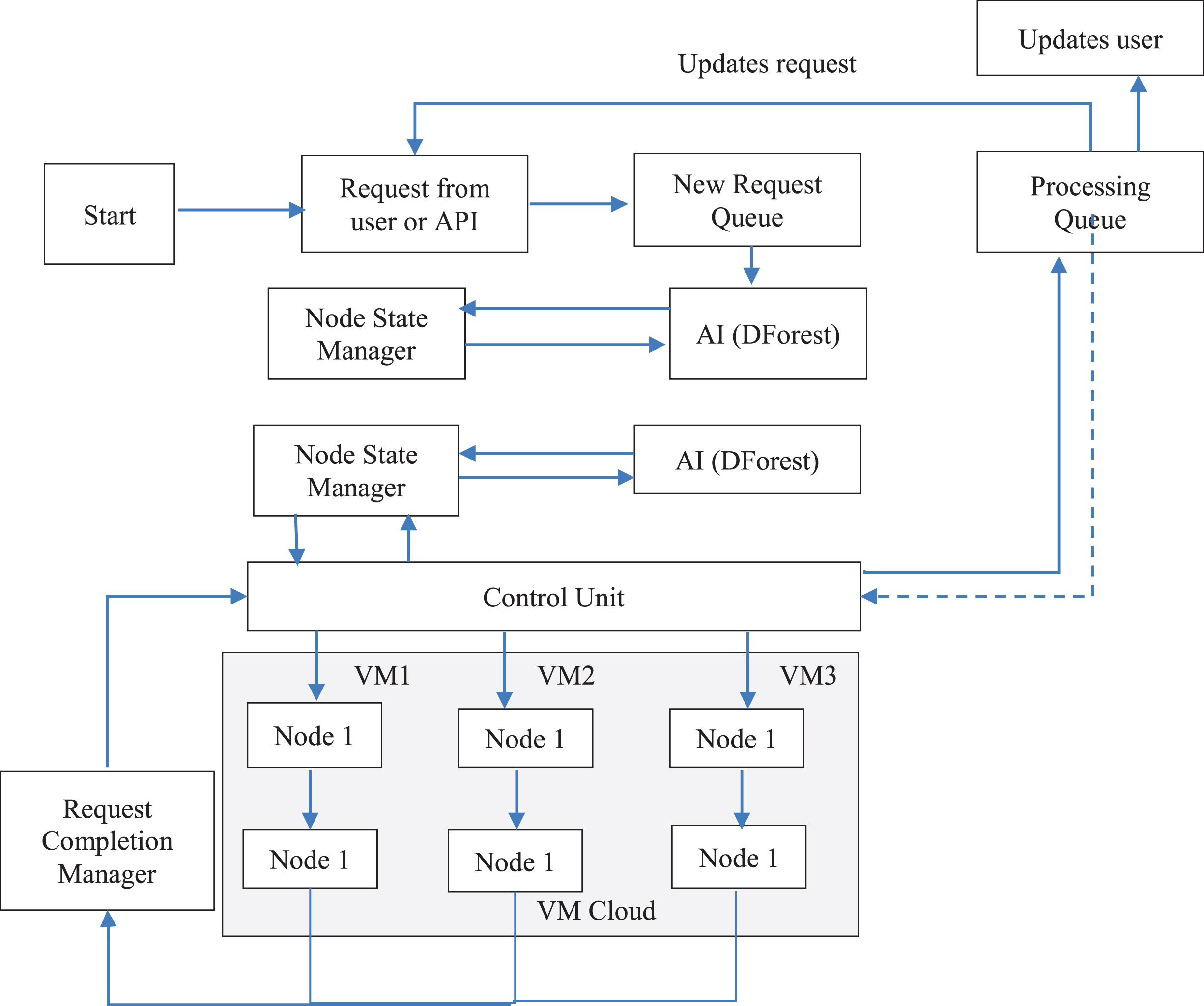
Load balancer architecture.

4.5.1 Request from API unit

Query raised by the API Group explains the weight balancer fundamental structure. Python Dispatch API code serves as an illustration of an application programming interface (API) that can be utilised to retrieve data from a network. API stands for application programming interface. It makes no difference what kind of security wall you have, if it comes with a certificate demonstrating that it is effective. This component will adjust the request so that it can be successfully distributed to the revised queue. A check is carried out by the request firewall of the API Unit to establish whether the file that is being requested is a bat file, a susceptible file, or a regular file. This check adds one more degree of safety to the overall system.

4.5.2 AI unit

AI strives to change workload environment and adapt continually improve QoS features, cut down on power usage, or lower overall infrastructure costs. AI includes a variety of machine learning, planning, reinforcement learning, and search methods. More intelligence is needed at many levels in present world data-intensive jobs with expanding and cloud deployments to give the best task scheduling decisions, VM migrations, etc. to optimise the aforementioned under different constraints. These limitations might include everything from bandwidth restrictions to SLAs or job deadline requirements for processing power.

A number of studies have been done with the goal of utilising AI approaches to raise the efficiency of fog and cloud systems. The best scheduling practises for clouds, virtualization techniques, and distribution systems, among other topics, are the subject of several studies. To optimise their goal functions, they employ search techniques like evolutionary supervised machine learning, algorithms, and even deep reinforcement learning. AI provides a lucrative approach to optimise big systems without enormous amounts of data with technological simplicity and efficiency by allowing automatic decision-making in place of human-encoded heuristics, resulting in more effective conclusions very quickly.

The study finds that the DFOREST algorithm has been pre-installed. The AI unit is comprised of two parts: the LSTM neural network and the DFOREST software.

4.6 Computational complexity

The computational complexity of the proposed AI-based load balancing program depends on various factors, including the specific machine learning algorithms used and the size of the dataset. Generally, the complexity can be broken down into the following aspects:

During the training phase of the machine learning model, the computational complexity mainly depends on the algorithm used (e.g., neural networks, decision trees, or support vector machines) and the size of the training dataset. More complex algorithms and larger datasets can lead to higher training time complexity.

Once the model is trained, the prediction phase involves processing incoming workload data and making load balancing decisions. The complexity of this phase depends on the efficiency of the trained model and the real-time prediction requirements.

The process of distributing workloads and resources across virtual machines involves making decisions based on the predictions from the AI-based load balancing algorithm. The complexity of this process is generally determined by the number of VMs, the workload distribution, and the allocation strategy.

The ability of the proposed AI-based solution to adapt to dynamic workload changes and make real-time load balancing decisions may introduce additional computational overhead. However, the efficiency of the model’s adaptability can also impact its overall complexity.

The machine learning-based AI solution for load balancing in cloud environments offers high accuracy and a thorough analysis of multiple algorithms. While the computational complexity may vary based on the specific implementation and algorithm used, the proposed method demonstrates promising results in efficiently handling load unbalancing and optimizing cloud server performance. Understanding the computational aspects is crucial for effectively implementing and deploying the AI-based load balancing program in real-world cloud environments. Further research and optimizations in the computational aspects can lead to even more efficient load balancing solutions in the future.

4.6.1 Big O notation

Just exponential operation of polynomials and sequencing is described using the large O microscopic designation, commonly referred to as the big O nomenclature. The big O acronym is utilized in the field of computer science to calculate and communicate the complexity of programs. What follows are the properties of the large O notation:

It sets the values of the coefficients of the calculation with the greatest development functional to one.

It must be at least 1.

It denotes a greater limit.

The big O notation estimates the amount of operations per procedure but does not account for connection notions. As a result, it does not satisfy N1. The big O designation counts the amount for commands performed by a technique, cannot the relationship actions with a relationship notion (which does not match N2). After moments, the large O notation may be used to complete N3. Due to the fact that the big O notation is written as a function of polynomials, project stakeholders can comprehend as well as contrast it (meets N4). Because large O notation is used for commands rather than interaction stages, it fails to satisfy N5. The big O notation is employed to analyze techniques prior to implementation.

5 Results and discussions

In this section, the research gathers information on performance counters in the network when it is in each of its three different load states: idle, normal, and overloaded. The server in the first scenario only processes standard HTTP requests, and its records are compiled, which guarantees that the data obtained has a high resolution. In the second scenario, the server does not process any HTTP requests at all. The second situation calls for the performance of two distinct test scenarios.

The machine learning-based AI solution for load balancing in cloud environments not only addresses load unbalancing but also offers significant practical managerial significance and potential applications across multiple domains. Its ability to enhance service reliability, optimize costs, improve QoS, and adapt to changing conditions makes it a promising solution for modern cloud computing. By considering practical applications and managerial implications, this approach holds the potential to revolutionize load balancing in cloud environments and beyond.

Figure 2(a) represents the dataset and pre-processing steps involved in cloud computing. In cloud computing, numerous sources, including Internet of Things (IoT) devices and social media platforms, produce a lot of data, and enterprise applications. This data needs to be processed and analysed to extract meaningful insights that can be used for decision-making. The first step data processing is data collection, where data is gathered from numerous sources and stored in a central repository such as a data lake. Once the data collected, the next step is data cleaning, where the data is checked for inconsistencies, errors, and missing values. Data cleaning makes the data better and ensures that it is suitable for analysis.

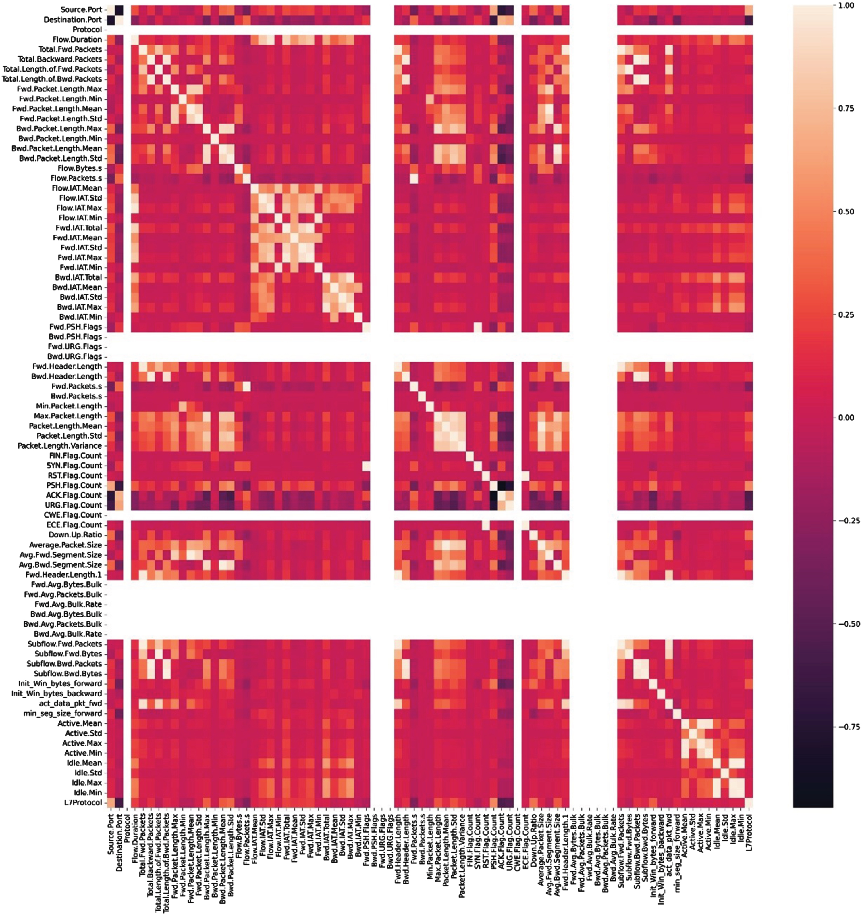
The research takes the feature dataset, which is made up of information that was generated by the network, and the research extract it from the graph that came before it, which demonstrates a more complicated data pattern. Figure 2b represents the correlation of variables in cloud computing. The degree to which two or more variables are related is demonstrated by the statistical measure known as correlation. Correlation analysis is used in cloud computing to determine the link between various variables and comprehend how they influence one another. The graphic shows a correlation matrix, which is a table listing the correlation coefficients between different pairs of variables. Perfectly negative correlations are represented by values of –1, zero, and one, respectively, while perfectly positive correlations are represented by values of 1.

Figure 2(c) represents a confusion matrix showing the accuracy with respect to different variables in cloud computing. Using the values in the confusion matrix, various metrics can be calculated to evaluate the accuracy of the machine learning model. Accuracy, precision, recall, and F1 score are some of these measurements. While accuracy is the percentage of correct forecasts, precision is the proportion of real positives among all predicted positives. Recall is defined as the percentage of true positives among all actual positives, and the F1 score is the harmonic mean of accuracy and recall. Overall, Fig. 2c highlights the importance of evaluating the accuracy of machine learning models in cloud computing. By using a confusion matrix and calculating numerous metrics, the performance of the model can be evaluated and optimized for better accuracy.

Fig. 2

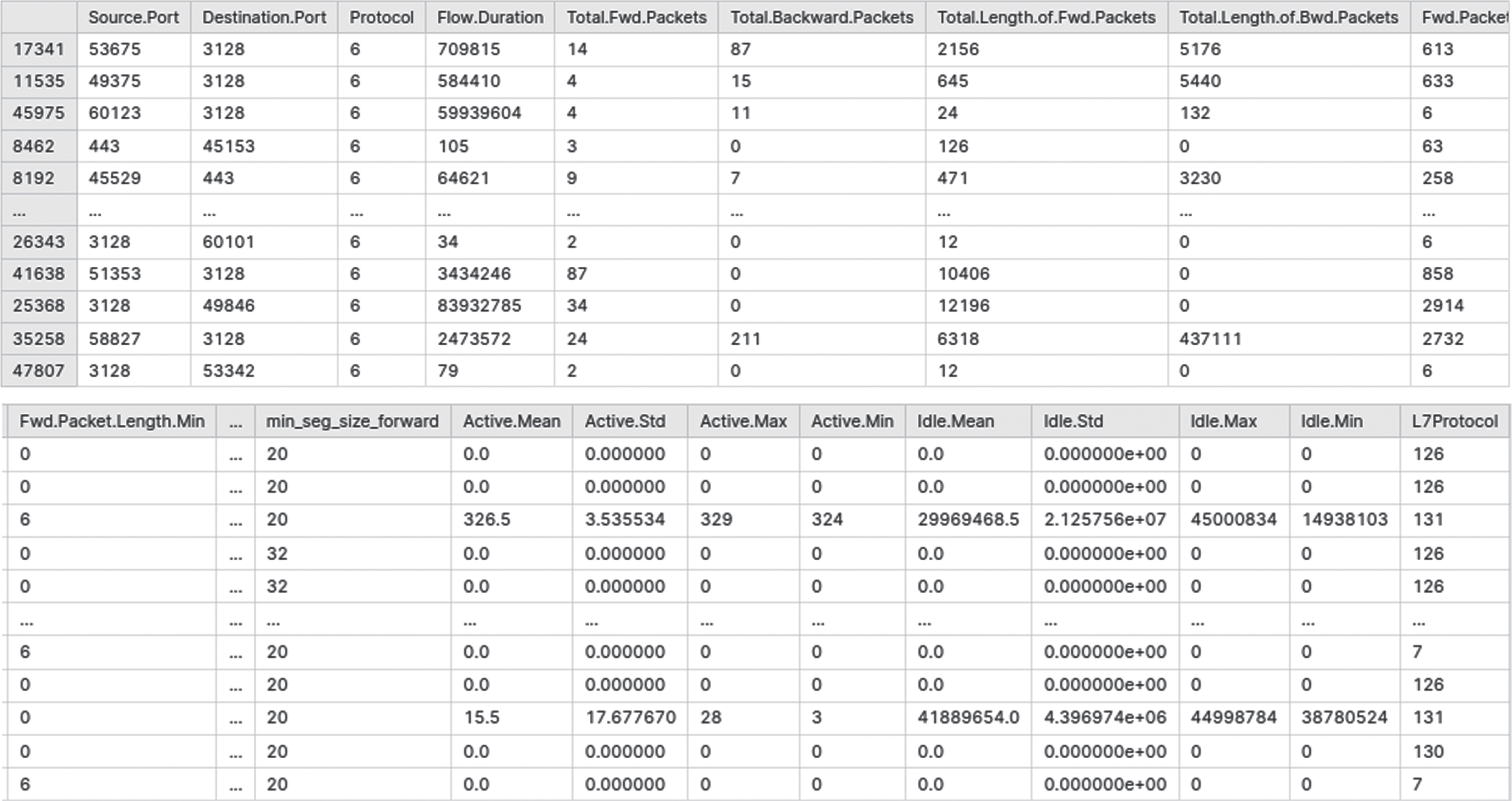
(a). Dataset and Pre-processing.

Fig. 2

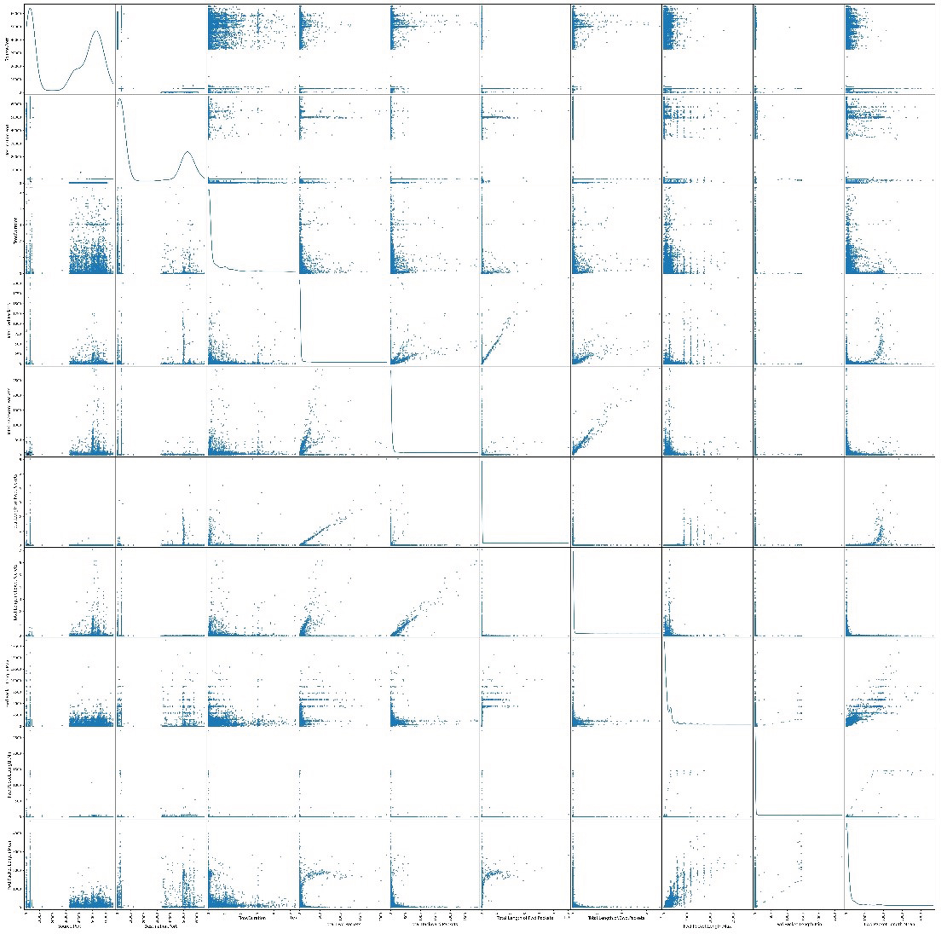
(b). Correlation of variables.

Fig. 2

(c). Confusion Matrix showing the accuracy w.r.t different variables.

A confusion matrix is a graphical representation of accuracy in connection to several different variables. This type of matrix can be found in psychology for us to achieve this objective, one of our primary focuses is on the development of a model that is underpinned by machine learning and has the capacity to make precise forecasts regarding the efficacy of load distribution for cloud services.

The next step that the research will take is to determine the machine learning algorithm that is most suitable for producing accurate forecasts regarding future processing units and attaining node parity across the entire network. This will be done by determining which machine learning algorithm is most suitable for producing accurate forecasts regarding future processing units. Our investigation will be directed by the data that the research collects, and the framework that the research give it will have a significant impact on how accurate our predictions are going to be.

The research has reorganised the dataset by segregating the features that are dependent on the class from the class itself while isolating those characteristics that are dependent on the class.to further improve the classifier precision, the research makes an attempt to extract the maximum quantity of useful information possible from the features. Because the real system only has four connections that can be used with the general performance counter, the research had to cut the original list of 36 features down to just the 20 that would be most useful for real-time monitoring.

Because of this limitation, the research was able to save a substantial amount of time and energy. Experiments in machine learning were conducted with our suggested algorithm as well as five other algorithms that have previously been shown to be successful against cache slide channel attacks. The results of these experiments were compared with the results of previous experiments. There is a total of five algorithms that were addressed, and they were as follows: Decision Tree, Random Forest, Naive Bayes, and Support Vector Machine.

Table 1 represents the prediction of the KNN algorithm. KNN is a type of supervised learning algorithm that can used for both regression and classification tasks. In KNN, the output value of a given input is based on the values of its neighbouring data points.

Table 1

Prediction of KNN

	Precision	Recall	F1-Score
Accuracy	0.94	0.96	0.95
Cross	0.93	0.94	0.95
Validation
Score
Avg. total	0.935	0.95	0.95

A KNN prediction graph Fig. 3 can be used visually evaluate accuracy of KNN algorithm. By comparing the predicted output values on scatter plot to the actual output values, it is possible to determine how accurate the algorithm is in predicting the output values for different input data points. Overall, a KNN prediction graph provides a useful visualization of the output values predicted by the KNN algorithm and can be used to evaluate and optimize the performance of the algorithm.

Fig. 3

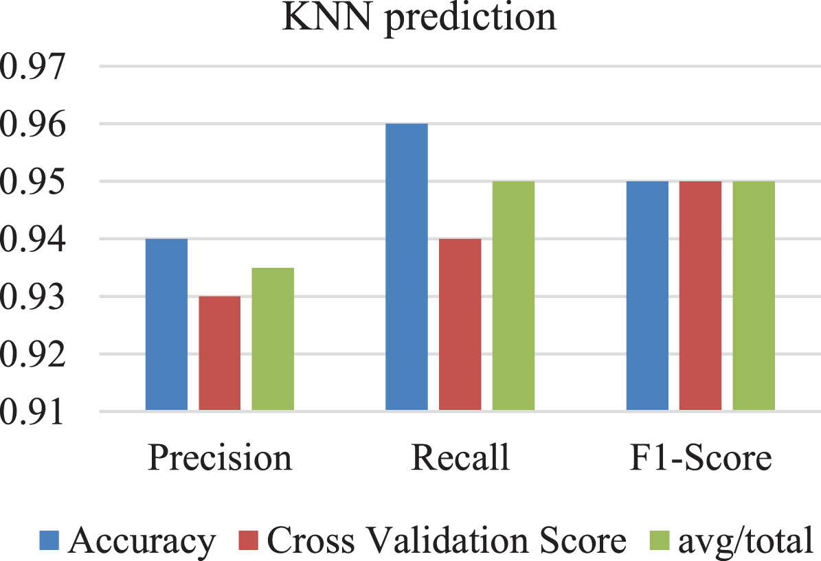
KNN prediction graph.

Table 2 represents the prediction of the RF algorithm. The supervised learning method RF may be applied to both classification and regression applications. Multiple decision trees are built during the training phase of RF, and their outputs are combined while the forecasting phase.

Table 2

Prediction of RF

	Precision	Recall	F1-Score
Accuracy	0.92	0.94	0.95
Cross	0.91	0.93	0.93
Validation
Score
Avg./total	0.91	0.93	0.94

The RF algorithm works by constructing multiple decision trees during training phase and then combining outputs of these trees during the prediction phase. In Fig. 4 an RF prediction graph, this process is represented by assigning each data point on the scatter plot to the predicted output value based on the combined output of the decision trees.

Fig. 4

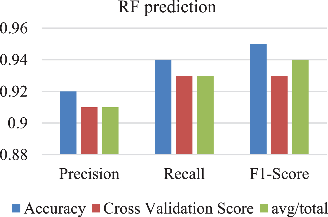
RF prediction graph.

The Table 3 shows performance metrics of SVM algorithm for a set of input data points. The performance metrics are represented by precision, recall, F1-score, accuracy, and cross-validation score. The “avg/total” row in the table represents the average or total values of the performance metrics across all the input data points. In this case, the average precision is 0.935, the average recall is 0.95, and the average F1-score is 0.95. Overall, Table 3 highlights the use of SVM for prediction tasks and the importance of evaluating the performance of the algorithm using different performance metrics. By analyzing the performance metrics, the performance of the algorithm can be optimized for better accuracy. SVM is known to be effective in dealing with both linear and non-linear data and provide a high level of accuracy in predicting outputs.

Table 3

Prediction of SVM

	Precision	Recall	F1-Score
Accuracy	0.94	0.96	0.95
Cross	0.93	0.94	0.95
Validation
Score
Avg./total	0.935	0.95	0.95

Based on their anticipated output values, the data points in an SVM prediction graph in Fig. 5 are categorised into several groups. The SVM method divides the data points into several classes by locating the best hyperplane. The data points nearest to the hyperplane, known as the support vectors, define the subspace.

Fig. 5

SVM prediction graph.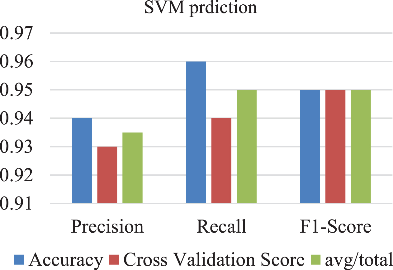

Table 4 shows that the DForest algorithm has achieved high accuracy in predicting the output values for the input data points, with an accuracy of 0.97 and a cross-validation score of 0.95. The precision and recall metrics are also high, indicating that the algorithm is performing well in identifying true positives and actual positives. The F1-score, however, is slightly lower than the other performance metrics, indicating that the algorithm may be better suited for precision or recall tasks rather than a balanced approach. Table 4 highlights the effectiveness of the DForest algorithm in predicting output values for classification tasks. By analyzing the performance metrics, the algorithm’s performance can be optimized for better accuracy. The high accuracy achieved by the DForest algorithm suggests that it is a reliable and efficient algorithm for classification tasks.

Table 4

Prediction of DForest

	Precision	Recall	F1-Score
Accuracy	0.97	0.97	0.94
Cross	0.95	0.95	0.94
Validation
Score
Avg./total	0.96	0.96	0.94

A DForest prediction Fig. 6 is a visualization tool that represents the predictions made by a Decision Forest (DForest) algorithm on a set of input data points. The input data points are typically represented on a scatter plot, with the x-axis representing one feature and the y-axis representing another feature.

Fig. 6

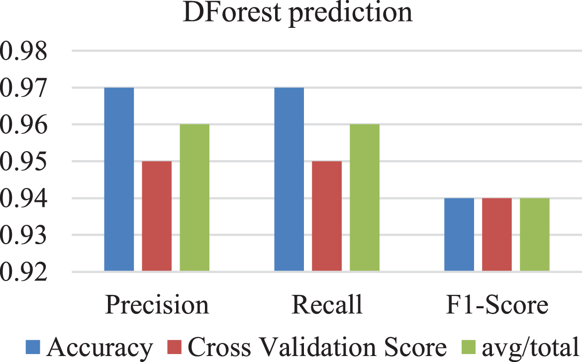
DForest prediction graph.

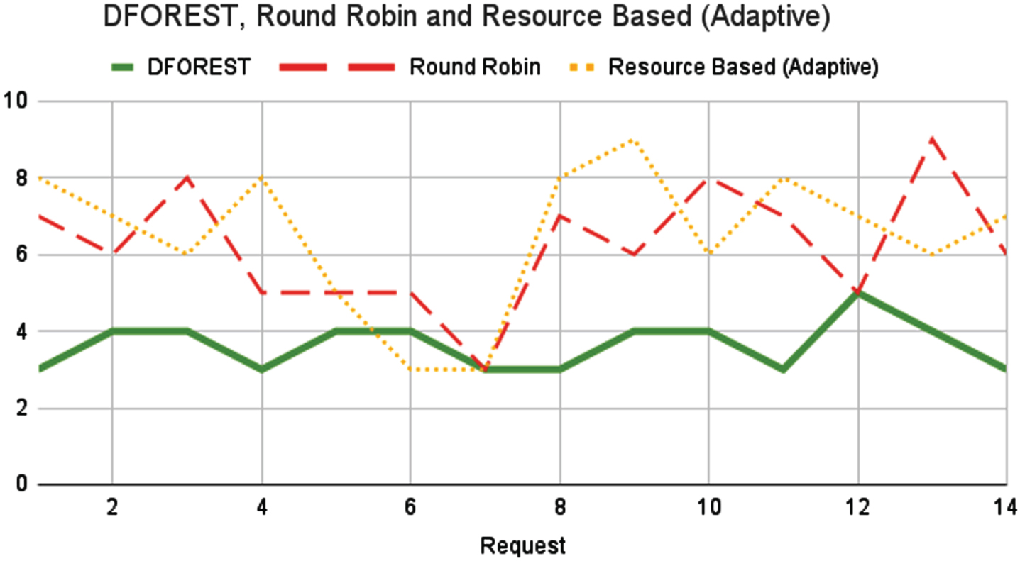
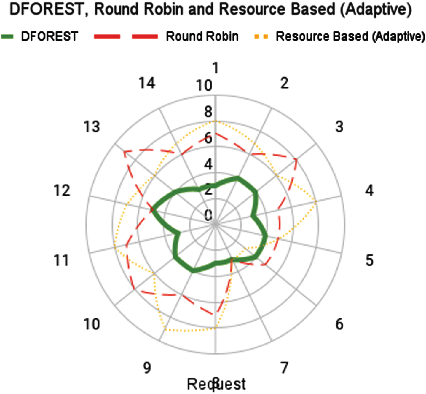
Table 5 shows the completion time of various machine learning models, including DForest, Round Robin, and Adaptive Algorithm, on 4 nodes for different input requests. The completion time is measured in seconds, and the input requests include data processing, data updation, and data retrieval.

Table 5

Completion time of Various Models on 4 nodes

Input	Request Type	DForest Routed Node	Completion time (s)	Round Robin Routed Node	Completion time (s)	Adaptive Algorithm Routed Node	Completion time (s)
1	Processing	3	3	1	7	4	8
2	Data updation	4	4	2	6	3	7
3	Data retrieval	1	4	3	8	4	6
4	Data retrieval	1	3	4	5	4	8
5	Processing	4	4	1	5	3	5
6	Processing	2	4	2	5	2	3
7	Data retrieval	3	3	3	3	4	3
8	Data updation	2	3	4	7	1	8
9	Processing	3	4	1	6	4	9
10	Processing	3	4	2	8	4	6
11	Processing	2	3	3	7	1	8
12	Data retrieval	1	5	4	5	3	7
13	Processing	3	4	1	9	3	6
14	Processing	4	3	2	6	4	7

The completion time graph Fig. 7 for the DForest, Round Robin, and Adaptive Algorithm routing algorithms would show the completion times for various input requests over time. The x-axis would represent time, and the y-axis would represent completion time in seconds. The graph would have separate lines for each routing algorithm, with each line representing the completion time of that algorithm over time. The completion times for the DForest, Round Robin, and Adaptive Algorithm routing algorithms would be plotted on the same graph so that they could be compared side by side.

Fig. 7

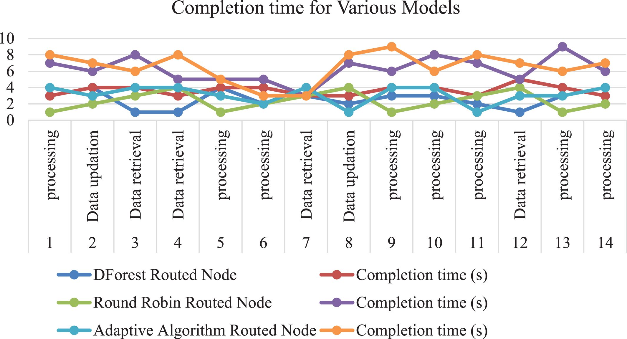
Various models time completion graph.

The Load Balancing Stability graph Fig. 8 with varying requests shows the stability of the load balancing system under different levels of workload. The x-axis represents the number of requests, while the y-axis represents stability of system, measured as standard deviation of response time. The graph would have a line that shows how the stability of load balancing system varies with number of requests. The line would start at a high point and gradually decrease as the number of requests increases. The line would show how the stability of the system changes as the workload increases. The graph would also have an upper and lower limit that represents the maximum and minimum stability of the system under different levels of workload. These limits would show the range of stability that is considered acceptable for the load balancing system. The Load Balancing Stability graph with varying requests is important because it helps cloud computing providers understand how their load balancing systems perform under different levels of workload.

Fig. 8

Load balancing stability.

The Fig. 9 that was just displayed provides an illustration of the dependability with which the weight was distributed among the nodes. This shows how load balancing remains stable even when the weights being carried out. By analyzing the stability of the system, providers can identify areas where the system is struggling and take steps to improve performance.

Fig. 9

Load Balancing Stability with varying request.

Figure 10 depicts the average response time (ART) values from the final set of simulations for all of the examined methodologies. Despite this, the proposed value of Art-242.0 (second-best ART) is superior to the rest of the work scheduling methodologies tested. The solution uses a load-balanced task mapping across the available resources, allowing all machines to be used equally, resulting in greater resource utilization, the shortest execution time for work scheduling, and a mild ART.

Fig. 10

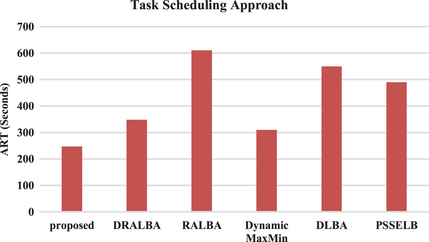
Task scheduling approach.

Figure 11 depicts the convergence graph of the HMWSO, ChOA (Chimp Optimization Algorithm), GTO (Artificial Gorilla Troops Optimizer), and AO (Aquila Optimizer) for the CVD dataset. The HMWSO method outperforms the ChOA, GTO, AO algorithms in terms of convergence. The suggested HMWSO algorithm enhances the ChOA, GTO, AO algorithm by including. The experimental findings with statistical analysis reveal that the HMWSO algorithm excels statistically. As seen by these graphs, HMWSO has the highest convergence rates for the majority of the benchmark functions, followed by ChOA, GTO, AO.

This article introduces a machine learning-based AI solution that thoroughly analyzes various load balancing algorithms available on the market. The research aims to address the challenges posed by load unbalancing and to design efficient AI-based load balancing programs. To achieve this, the article emphasizes the need to understand the advantages and disadvantages of current methodologies.

Fig. 11

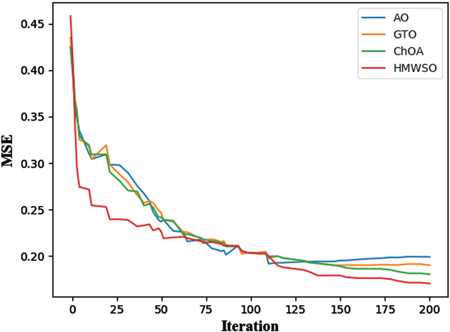
Using convergence curve for find best score.

5.1 Advantages

The AI-based approach effectively distributes workloads across VMs, reducing the chances of overloading or underloading, thus enhancing overall system performance.

The algorithm demonstrates scalability, allowing it to adapt to varying workloads and cloud server environments efficiently.

The AI-based solution can dynamically adjust load balancing strategies in real-time based on changing workload demands, ensuring optimal resource utilization at all times.

Leveraging machine learning techniques, the algorithm achieves better load prediction accuracy, leading to more accurate and informed resource allocation decisions.

The efficient load balancing reduces server response time and minimizes latency, resulting in improved user experience.

5.2 Disadvantages compared to the existing methods

The machine learning-based algorithm requires initial training, which may introduce some overhead during the learning phase.

While the proposed algorithm aims to optimize resource allocation, it may consume additional computational resources during load prediction and distribution.

The success of the AI-based approach heavily relies on the availability and quality of the dataset used for training. Inadequate or biased data may lead to suboptimal load balancing decisions.

The proposed algorithm may encounter difficulties in generalizing to new, unseen workload patterns, especially if the training dataset lacks diversity.

The algorithm’s performance could be sensitive to the duration and characteristics of the training period, impacting its ability to adapt to sudden workload changes.

To facilitate a better understanding for the reader, the article provides comprehensive details of the experimental setup, including the datasets used, evaluation metrics, and hardware configurations. It thoroughly analyzes the results obtained from experiments, emphasizing the strengths and limitations of the proposed AI-based load balancing algorithm when compared to existing methods. The insights gained from these analyses contribute to a better understanding of the practical implications and potential real-world applications of the proposed solution.

6 Conclusions

In this research, DForest model is used to balance the load in cloud for different queries over 4 different nodes. Several different algorithms and methods were combined to achieve a better load balancing stability. Despite this, the problem with the ML is the most encouraging one throughout the entire CC system. Several different algorithms and methods were combined to create a hybrid system that provided good cloud service, complexity, and effective use of resources at a low cost to find a solution to this computing problem. The article’s proposed machine learning-based AI solution for load balancing in cloud environments presents a solid foundation for future research. Addressing the identified future scope and open research questions could pave the way for more efficient, adaptive, and intelligent load balancing strategies, contributing to the continuous improvement of cloud server performance and resource management.

References

Kruekaew

and Kimpan

, Multi-Objective Task Scheduling Optimization for Load Balancing in Cloud Computing Environment Using Hybrid Artificial Bee Colony Algorithm With Reinforcement Learning, IEEE Access 10 (2022), 17803–17818. doi: 10.1109/ACCESS.2022.3149955.

Tong

, Chen

, Deng

, Li

and Li

, A scheduling scheme in the cloud computing environment using deep Q-learning, Inf. Sci. 512 (2020), 1170–1191. doi: 10.1016/j.ins.2019.10.035.

Shu

, Cai

and Xiong

N.N.

, Research on strong agile response task scheduling optimization enhancement with optimal resource usage in green cloud computing, Future Gener. Comput. Syst. 124 (2021), 12–20. doi: 10.1016/j.future.2021.05.012.

Zhang

, Design and application of fog computing and Internet of Things service platform for smart city, Future Gener. Comput. Syst. 112 (2020), 630–640. doi: 10.1016/j.future.2020.06.016.

Berntzen

and Wong

S.I.

, Autonomous but Interdependent: The Roles of Initiated and Received Task Interdependence in Distributed Team Coordination, Int. J. Electron. Commer. 25(1) (2021), 7–28. doi: 10.1080/10864415.2021.1846851.

Asghari

, Sohrabi

M.K.

and Yaghmaee

, Task scheduling, resource provisioning, and load balancing on scientific workflows using parallel SARSA reinforcement learning agents and genetic algorithm, J. Supercomput. 77(3) (2828), 2800–2828. doi: 10.1007/s11227-020-03364-1.

Hossain

M.R.

et al. A scheduling-based dynamic fog computing framework for augmenting resource utilization, 36, Simul. Model. Pract. Theory 111 (2021), 102336. doi: 10.1016/j.simpat.2021.102336.

Nanjappan

and Albert

, Hybrid-based novel approach for resource scheduling using MCFCM and PSO in cloud computing environment, Concurr. Comput. Pract. Exp. 34(7) (2022). doi: 10.1002/cpe.5517.

Xingjun

, Zhiwei

, Hongping

and Mohammed

B.O.

, A new fuzzy-based method for load balancing in the cloud-based Internet of things using a grey wolf optimization algorithm, Int. J. Commun. Syst. 33(8) (2020), e4370. doi: 10.1002/dac.4370.

10.

Paya

and Marinescu

D.C.

, Energy-Aware Load Balancing and Application Scaling for the Cloud Ecosystem, IEEE Trans. Cloud Comput. 5(1) (2017), 15–27. doi: 10.1109/TCC.2015.2396059.

11.

Zhao

, Yang

, Wei

, Ding

, Hu

and Xu

, A Heuristic Clustering-Based Task Deployment Approach for Load Balancing Using Bayes Theorem in Cloud Environment, IEEE Trans. Parallel Distrib. Syst. 27(2) (2016), 305–316. doi: 10.1109/TPDS.2015.2402655.

12.

Devaraj

A.F.S.

, Elhoseny

, Dhanasekaran

, Lydia

E.L.

and Shankar

, Hybridization of firefly and Improved Multi-Objective Particle Swarm Optimization algorithm for energy efficient load balancing in Cloud Computing environments, J. Parallel Distrib. Comput. 142 (2020), 36–45. doi: 10.1016/j.jpdc.2020.03.022.

13.

Thein

, Myo

M.M.

, Parvin

and Gawanmeh

, Reinforcement learning based methodology for energy-efficient resource allocation in cloud data centers, J. King Saud Univ. –Comput. Inf. Sci. 32(10) (2020), 1127–1139. doi: 10.1016/j.jksuci.2018.11.005.

14.

Yang

M.-J.

, Energy-efficient cloud data center with fair service level agreement for green computing, Clust. Comput. 24(4) (2021), 3337–3349. doi: 10.1007/s10586-021-03342-z.

15.

Sohani

and Jain

S.C.

, A Predictive Priority-Based Dynamic Resource Provisioning Scheme With Load Balancing in Heterogeneous Cloud Computing, IEEE Access 9 (2021), 3349–62664. doi: 10.1109/ACCESS.2021.3074833.

16.

Mishra

S.K.

, Sahoo

and Parida

P.P.

, Load balancing in cloud computing: A big picture, J. King Saud Univ. –Comput. Inf. Sci. 32(2) (2020), 149–158. doi: 10.1016/j.jksuci.2018.01.003.

17.

, Parthiban

Quasi Oppositional Dragonfly Algorithm for Load Balancing in Cloud Computing Environment, In Review, preprint, (2021). doi: 10.21203/rs.3.rs-330652/v1.

18.

Karimzadeh Parizi

, Keynia

and Khatibi Bardsiri

, Woodpecker Mating Algorithm WMA): a nature-inspired algorithm for solving optimization problems, Int. J. Nonlinear Anal. Appl. 11(1) (2020), doi: 10.22075/ijnaa.2020.4245.

19.

Karimzadeh Parizi

, Keynia

and Khatibi Bardsiri

, OWMA: An improved self-regulatory woodpecker mating algorithm using opposition-based learning and allocation of local memory for solving optimization problems, J. Intell. Fuzzy Syst. 40(1) (2021), 919–946. doi: 10.3233/JIFS-201075.

20.

Parizi

M.K.

, Keynia

and Bardsiri

A.K.

, HSCWMA: A New Hybrid SCA-WMA Algorithm for Solving Optimization Problems, Int. J. Inf. Technol. Decis. Mak. 20(02) (2021), 775–808. doi: 10.1142/S0219622021500176.

21.

Zhang

, Li

and Parizi

M.K.

, HWMWOA: A Hybrid WMA–WOA Algorithm with Adaptive Cauchy Mutation for Global Optimization and Data Classification, Int. J. Inf. Technol. Decis. Mak. 22(04) (2023), 1195–1252. doi: 10.1142/S0219622022500675.

22.

Gong

and Karimzadeh Parizi

, , GWMA: the parallel implementation of woodpecker mating algorithm on the GPU, J. Chin. Inst. Eng. 45 (2022), 1–13. doi: 10.1080/02533839.2022.2078418.

23.

Wang

and Guan

, An adaptive dynamic feedback load balancing algorithm based on QoS in distributed file system, J. Commun. Inf. Netw. 2(3) (2017), 30–40. doi: 10.1007/s41650-017-0029-3.

24.

Shahdi-Pashaki

, Teymourian

and Tavakkoli-Moghaddam

, New approach based on group technology for the consolidation problem in cloud computing-mathematical model and genetic algorithm, Comput. Appl. Math. 37(1) (2018), 693–718. doi: 10.1007/s40314-016-0362-4.

25.

Renggli

, Ashkboos

, Aghagolzadeh

, Alistarh

, Hoefler

SparCML: high-performance sparse communication for machine learning, in Proceedings of the International Conference for High Performance Computing, Networking, Storage and Analysis, Denver Colorado: ACM (2019), 1–15. doi: 10.1145/3295500.3356222.

26.

Andrade

and Nogueira

, Dependability evaluation of a disaster recovery solution for IoT infrastructures, J. Supercomput. 76(3) (2020), 1828–1849. doi: 10.1007/s11227-018-2290-0.

27.

Nabi

, Ibrahim

and Jimenez

J.M.

, DRALBA: Dynamic and Resource Aware Load Balanced Scheduling Approach for Cloud Computing, IEEE Access 9 (2021), 61283–61297. doi: 10.1109/ACCESS.2021.3074145.

28.

Ibrahim

et al. An In-Depth Empirical Investigation of State-of-the-Art Scheduling Approaches for Cloud Computing, IEEE Access 8 (2020), 128282–128294. doi: 10.1109/ACCESS.2020.3007201.

29.

Mishra

S.K.

, Sahoo

and Parida

P.P.

, Load balancing in cloud computing: A big picture, J. King Saud Univ. –Comput. Inf. Sci. 32(2) (2020), 149–158. doi: 10.1016/j.jksuci.2018.01.003.

30.

Cito

J.R.

, Gotowka

, Leitner

, Pelette

, Suljoti

, Dustdar

IDENTIFYING WEB PERFORMANCE DEGRADATIONS THROUGH SYNTHETIC AND REAL-USER MONITORING”.

31.

Zhang

, Li

, Zheng

and Li

, Contention-Aware Reliability Efficient Scheduling on Heterogeneous Computing Systems, IEEE Trans. Sustain. Comput. 3(3) (2018), 182–194. doi: 10.1109/TSUSC.2017.2743499.

32.

Jena

U.K.

, Das

P.K.

and Kabat

M.R.

, Hybridization of meta-heuristic algorithm for load balancing in cloud computing environment, J. King Saud Univ. –Comput. Inf. Sci. 34(6) (2022), 2332–2342. doi: 10.1016/j.jksuci.2020.01.012.

Optimizing cloud resource allocation: A long short-term memory and DForest-based load balancing approach

Abstract

Keywords

1 Introduction

1.1 Key contribution

1.2 Limitations of the study

2 Related works

3 Problem statement

4 Proposed method

4.1 Task assignment

4.3 Information storage in long short-term memory (LSTM) networks

4.4.1 Random forest classifier

4.4.3 Proposed dforest algorithm

4.5.2 AI unit

4.6 Computational complexity

4.6.1 Big O notation

5 Results and discussions

5.2 Disadvantages compared to the existing methods

6 Conclusions

References