Sage Journals: Discover world-class research

Abstract

Trailing suction hopper dredger is a kind of hydraulic dredger, it has the characteristics of self-propelled, selfloading, self-dredging, self-unloading, it is the main force in dredging and blowing works, it is widely used in the world, it can be said that where there is a big dredging project where there is a trailing suction hopper dredger’s figure. The loading optimization process of trailing suction hopper dredger contains a lot of dredging parameters related to soil type, and the soil type under different working conditions is not very clear. In this study, we present a hybrid optimization technique based on simulated annealing and multi-population genetic algorithm to enhance the loading efficiency of a trailing suction hopper dredger and to examine the variation of dredged soil parameters. The soil parameters of the spoil hopper deposition model were estimated using this hybrid optimization algorithm. The experimental results show that the soil parameters are successfully estimated and verified by our measured construction data of a trailing suction hopper dredger. In addition, our proposed method has the highest accuracy of soil parameter estimation, the fastest algorithm convergence, and excellent robustness compared to the other three intelligent optimization methods. In addition, our method successfully avoids the phenomenon of premature convergence that usually occurs in traditional genetic algorithms, and the parameters show strong adaptability to different vessels under the same dredging area.

Keywords

Trailing suction hopper dredger spoil hopper deposition model simulated annealing and multi-population genetic algorithm soil parameters estimation

1 Introduction

As an engineering vessel incorporated with high-technology and high-value-added, dredger is performing an increasingly crucial role in many dredging engineering applications, such as the construction and maintenance of waterways and ports, environmental dredging of rivers and lakes, land blowing and sand mining in deep-sea [1]. Compared with other types of vessels, trailing suction hopper dredgers (TSHDs) possess advantages of self-propulsion, self-loading and unloading, deep dredging, and high flexibility, etc. However, in the construction of the TSHD, the dredged soil differences often involve real-time dynamic changes in soil parameters, which are difficult to be examined by measuring devices or empirical formulas. This causes difficulties in optimizing the TSHD loading process and developing intelligent auxiliary decision-making systems. Therefore, feasible and applicable methods need to be put forward for accurate and effective estimation of soil parameters in the spoil hopper deposition model.

Before soil parameters estimation, a mathematical model representing the sedimentation and overflow process in spoil hopper of TSHD needs to be constructed. To this end, many well-known scholars and institutions have conducted in-depth and extensive researches. For example, the study [2] pioneered the classical sedimentation model of mud unloading tanks as early as 1936 by utilizing an ideal sedimentation tank to simulate the sedimentation process in the mud unloading tanks of TCC. Subsequently, the model proposed by Camp was refined and improved. A novel model based on the concentration distribution of open channel flows was then proposed in study [3]. In order to improve predictions of overflow losses and deposition efficiency, studies [4, 5] introduced additional features that hinder deposition. Camp’s model was used in the tests of Studies [6, 7] to combine sediment particle kinetic calculations and analyze overflow loss and overflow density of the cement mixture as it enters the hopper.

The study [8 , 10] developed a one-dimensional approximate settlement model and a two-dimensional more complex settlement model to verify whether the structure of the disposal hopper affects its loading efficiency. The study [11] developed three mathematical models (i.e., linear, exponential, and pelagic) for overflow density calculation. On the basis of real-time shipping data, it was discovered that the water-layer model outperformed all others in simulating the distribution of mud and sand in the spoil hopper.Study [12] derived a simplified model of dump hopper deposition by exploring the factors affecting sediment bed uplift during sediment deposition. Study [13] investigated the non-cohesive sediment scour by using the computational fluid dynamics (CFD) method and empirical equations, and developed a two-dimensional mathematical model to reveal the deposition process of the loading compartment of the table sediment field. In order to better simulate the near-field behavior of the sediment overflow plume, the study [14] constructed a more accurate CFD model. However, in order to overcome the disadvantages of the CFD model such as time-consuming computation, he proposed a semi-analytical parametric model, which can well reproduce the diffusion process of the near-field cement mixture simulated by the CFD model. Study [15] combined the large eddy simulation (LES) of turbulence with the volume-of-fluid (VOF) method of two-phase transport to accurately capture detailed information of the overflow flow field near the hull of a ship and to characterize the advective and diffusive overflows of the cement mixture.

After the construction of the hopper deposition model of TSHD, the soil parameters of the model need to be estimated. Study [16] used Pattern Search (PS) algorithm to estimate the dredging parameters of soil types, although the algorithm is simple, it is a serial process and the search efficiency is low. Studies [17] used Genetic Algorithm (GA) to estimate the soil parameters of the dump hopper model during loading, which showed higher accuracy compared to the traditional pattern search method, however, the algorithm tended to converge to a locally optimal solution. Studies [18] applied the standard particle filtering (PF) and feedback particle filtering (FPF) methods to soil parameter estimation, and the results showed that FPF estimated soil parameters more accurately. Subsequently, studies [19, 20] attempted to use other filters, such as the Reduced Order Particle Filter (ROPF) and Improved Saturated Particle Filter (ISPF) for online estimation of soil particle size in loaded sediments.

To overcome the challenges in estimating soil parameters in the loading process of the TSHD, based on previous studies, we propose a mixed algorithm, the Simulated Annealing and Multiple Population Genetic Algorithm (SAMPGA) as a result of the combination of Simulated Annealing (SA) capable of local search and Multiple Population Genetic Algorithm (MPGA), a robust algorithm for global search. This hybrid algorithm is applied to estimate the soil parameters of a spoil hopper sedimentation model. With soil parameters estimated, important variables such as overflow density as well as sand bed height in the loading process of TSHD are predicted by the spoil hopper deposition model proposed by Braaksma. This study hopefully contributes to optimizing the loading process of the TSHD, improving dredging performance and efficiency, and shortening the construction cycle.

2 Loading process spoil hopper deposition model

When the TSHD sails to construction water, the drag head is used to break up the soil and excavate the mud and sand on the water bottom. The mixture of mud and water is sucked by the mud pump through the suction pipe into the spoil hopper for sedimentation, and the loading of sediment is increased by overflowing. The suction pipe is then put away and the loading process stops when the spoil hopper is full. This loading process affects the dredging yields and efficiency of the ship. The schematic diagram of a TSHD is depicted in Fig. 1.

Fig. 1

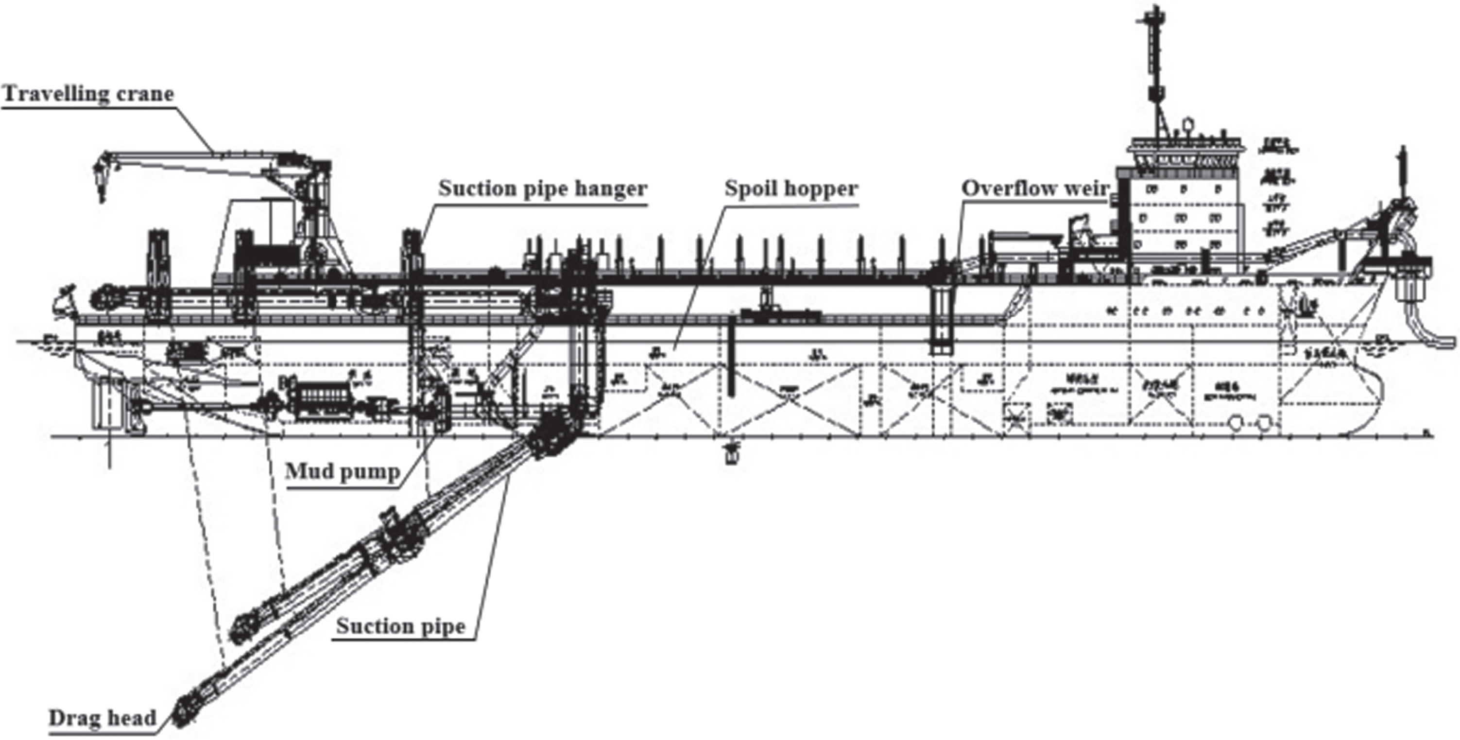
The schematic diagram of a TSHD.

The drag head excavation model, the mud pump pipeline transport model and the spoil hopper sedimentation model together constitute the hopper loading optimization mechanism model, as shown in Fig. 2. Since the spoil hopper deposition optimization reflects more of dredger output and efficiency, and since the loading of mud and sand into the spoil hopper is complex and involves more physical variables, this paper focuses mainly on the spoil hopper deposition model [21].

Fig. 2

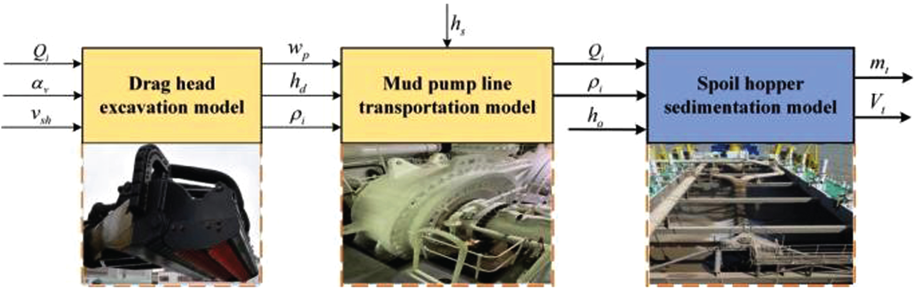
The relational model of excavation, transport and sedimentation process.

As it can be observed in Fig. 2, density ρ_i of the mixture of water-mud sucked in by the drag head is affected by speed v_sh of the ship and the flow rate of the mixture Q_i. Through controlling the opening degree α_v of the drag head inlet valve, density ρ_i of the sucked in mixture can be reduced to prevent cavitation in the mud pump. With the speed w_p of mud pumping, the water-mud mixture is transported into the spoil hopper for settlement at flow rate Q_i and density ρ_i via the pipeline, and the pressure reduction in the pipeline is in agreement with the variation of the water-mud mixture’s density ρ_i, the underwater position h_d of mud pump and dredging depth h_z. By manipulating the overflow weir height h_o, the mass m_t and volume V_t of the mixture loaded into the spoil hopper can be adjusted. At this point, input in the spoil hopper deposition model includes inlet mixture flow rate Q_i and density ρ_i, overflow weir height h_o; output of the model includes total weight m_t and volume of the spoil hopper load V_t.

The main part of sediment deposition in the spoil hopper is illustrated in Fig. 3. The water-mud mixture flows into the spoil hopper at a flow rate of Q_i and with a density of ρ_i. The sediment settles at the bottom of the spoil hopper at a flow rate of Q_s. With the time passing, a sand bed at the height h_s and with a density ρ_s gradually forms. In the middle of the spoil hopper, a layer of undeposited mixture at the height of (h_t - h_s - h_w) and with a mean density of ρ_m is formed. Meanwhile, the sedimentation of mud and sand particles directs the water flow towards the opposite direction at the flow rate Q_w, thus forming a small and thin layer of water at the height h_w and with the density ρ_w above the liquid surface of the spoil hopper. When the height h_t of the water-mud mixture in the spoil hopper exceeds the overflow weir height h_o, the top layer of low-density mixture flows out of the spoil hopper from the overflow weir at a flow rate of Q_o and with a density of ρ_o, causing the spoil hopper to slow down the loading of sediment [22]. The mass of hopper loading and overflow losses are not only greatly influenced by the soil type, but also depend on the magnitude of the inlet mixture flow rate Q_i and density ρ_i.

Fig. 3

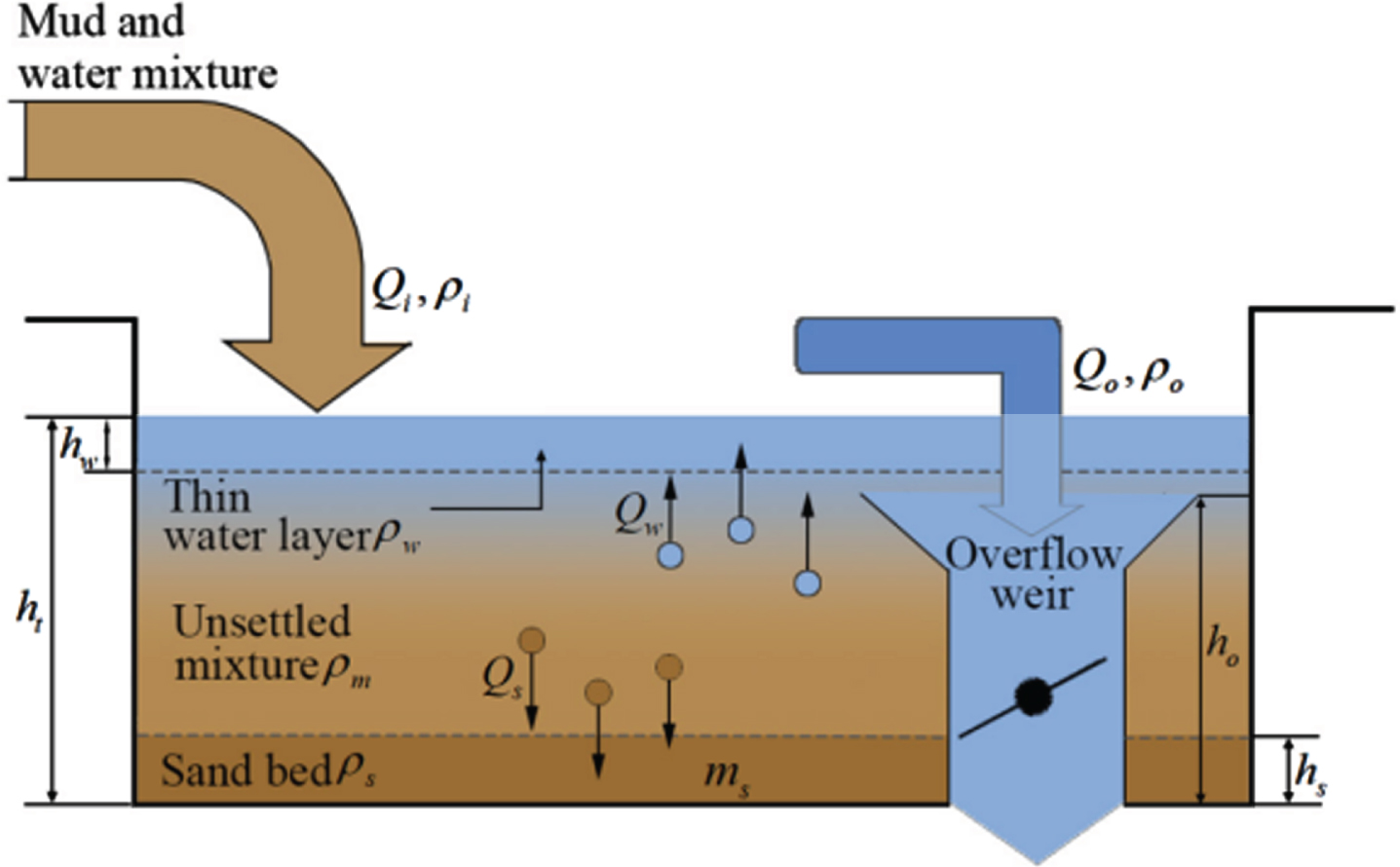
The schematic diagram of spoil hopper sediment deposition and overflow process.

In order to optimize the loading process, a spoil hopper deposition model incorporated with the equilibrium equation for the mass of the hopper, the overflow flow rate, and the density is developed.

2.1 Spoil hopper mass balance equation

The overflow density cannot be obtained by direct sensor measurements. The distribution of the density of this mixture within the spoil hopper is a decreasing function of height and changes continuously with the loading process. In this paper, a pelagic model, which is closely related to the soil parameters, is used to estimate the overflow density values and to verify the accuracy of the soil parameter estimates by the quality of the loaded pods.

The spoil hopper deposition model can be expressed by the mass and volume balance equations in equation (1): ${\begin{matrix} d V_{t} = (Q_{i} - Q_{o}) d_{t} \\ d m_{t} = (Q_{i} ρ_{i} - Q_{o} ρ_{o}) d_{t} \end{matrix}$ (1)

Where V_t and m_t represent the volume and mass of the mixture in the spoil hopper respectively; Q_i and ρ_i denote the flow rate and density of the mixture when loaded into the spoil hopper; Q_o and ρ_o refer to the overflow flow rate and density of the mixture, respectively. The above equation reflects the equilibrium between the volume and mass of the loaded sediment over a period of time in the spoil hopper.

2.2 Overflow rate

When the water-mud mixture flows out via the overflow weir, Q_o can be expressed as: $Q_{o} = k_{o} max (h_{t} - h_{o}, 0)^{\frac{3}{2}}$ (2)

Where h_t and h_o represent the spoil hopper liquid level and overflow weir height, respectively. k_o is a nonconstant parameter varying according to the shape and circumference of the overflow weir.

2.3 Overflow density

On the top of the sand bed, the density of water-mud mixture in the spoil hopper shows a decreasing trend with increased height, so the segmentation function of the water-layer model can be used to represent the mixture density distribution in the spoil hopper, as depicted in Fig. 4.

Fig. 4

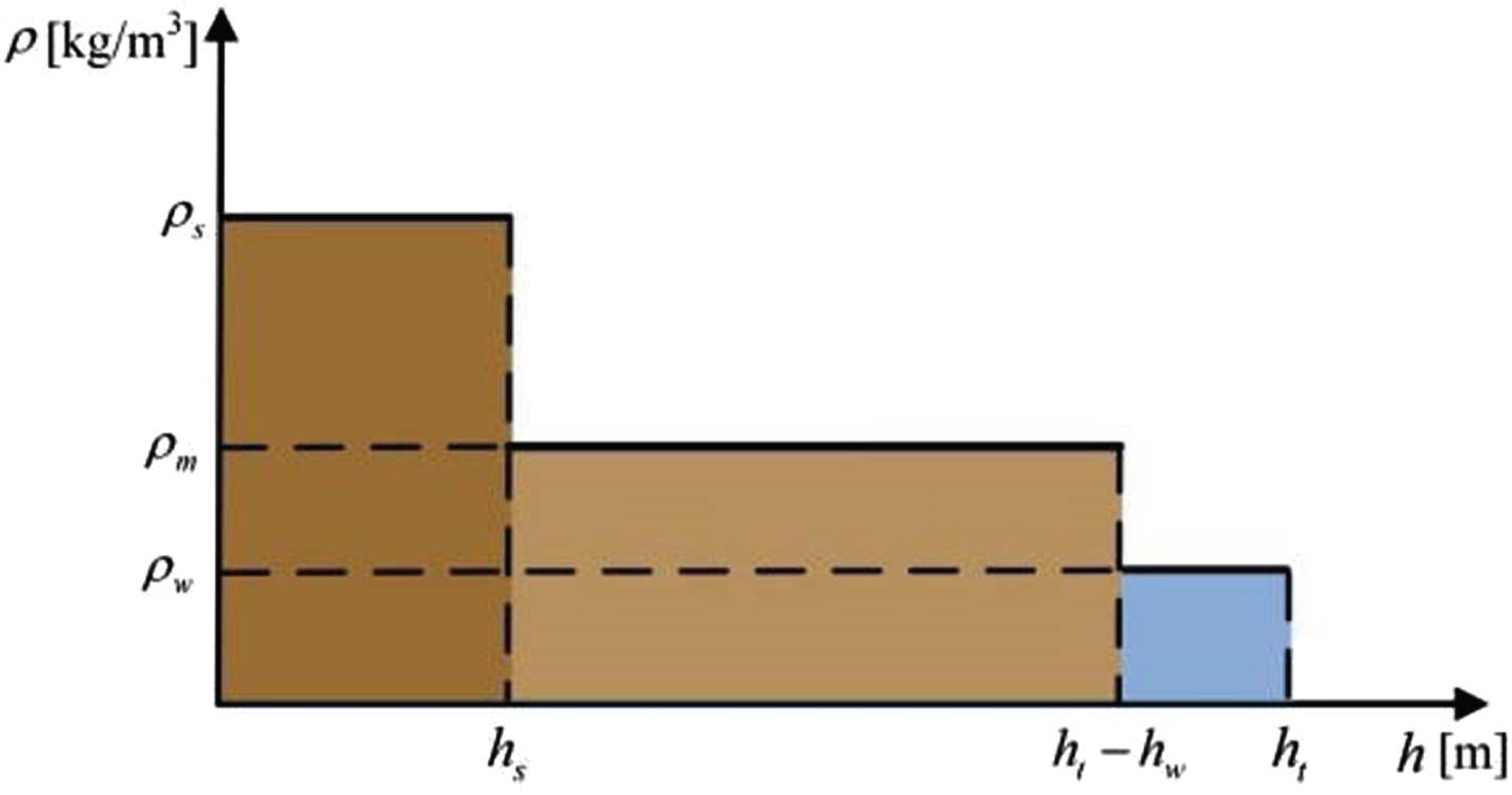
Density distribution diagram of water layer model.

The horizontal and vertical coordinates in the above figure indicate liquid the surface height h in the spoil hopper and density ρ of water-mud mixture, respectively. The density distribution of the mixture in the spoil hopper can be divided into upper water layer, middle water-mud mixture layer and lower sand bed layer. Upper layer at the height from (h_t - h_w) to h_t is the water with density ρ_w, middle layer at the height from h_s to (h_t - h_w) is slurry with an average density of ρ_m, and lower layer at the height h_s and below is a sand bed with density ρ_s. Therefore, the formula of the water-layer model function can be expressed as follows. ${\begin{matrix} ρ_{s} 0 < h < h_{s} \\ ρ_{m} h_{s} < h < h_{t} - h_{w} \\ ρ_{w} h_{t} - h_{w} < h < h_{t} \end{matrix}$ (3)

Above the sand bed layer, the average density ρ_ms of entire water-mud mixture can be solved according to the following equation: $ρ_{ms} = \frac{ρ_{s} (m_{t} - m_{s})}{V_{t} ρ_{s} - m_{s}}$ (4)

Where ρ_s and m_s denote the density and mass of the sand bed formed at the bottom of the spoil hopper, separately; m_s can be calculated by the sand bed mass balance equation (5). $d m_{s} = Q_{s} ρ_{s} d_{t}$ (5)

Q_s is the settling flow rate of mud-sand in the hopper, which can be computed by multiplying the scouring function f_e of mud and sand movement on the sand bed with the process function f_s of mud and sand settling in the hopper, as shown in equation (6). $\begin{matrix} Q_{s} = f_{e} \cdot \end{matrix} f_{s}$ (6)

The scouring function f_e depicts the scouring effect of upper low-density mixture overflowing on the sand bed at the hopper’s bottom when water-mud mixture in the spoil hopper reaches the height of the overflow weir. $\begin{matrix} f_{e} = max \end{matrix} (1 - {(\frac{Q_{o}}{k_{e} h_{m}})}^{2}, 0)$ (7)

Where k_e is the scouring coefficient which can be influenced by soil type, h_m is the height of the water-mud mixture over the sand bed layer, which can be expressed as: $\begin{matrix} h_{m} = \end{matrix} h_{t} - h_{s}$ (8)

The settling function f_s describes the process by which mud and solid sand particles suspending in the mixture above the sand bed gradually settle down at the spoil hopper’s bottom. $\begin{matrix} f_{s} = \end{matrix} A v_{s 0} \frac{ρ_{m} - ρ_{w}}{ρ_{s} - ρ_{m}} {(\frac{ρ_{q} - ρ_{m}}{ρ_{q} - ρ_{w}})}^{β}$ (9)

Where ρ_w and ρ_q are the densities of water and quartz, respectively, v_{s
_o} is the undisturbed settling velocity of sediment particles, β is the hindered settling coefficient, and A represents the horizontal area of the spoil hopper where mud and sand settle, which can be obtained by (10) equation. $\begin{matrix} A = \end{matrix} \frac{V_{t} - V_{s}}{h_{m}}$ (10)

Where V_s is the volume of the sand bed, which can be expressed as: $\begin{matrix} d V_{s} = \end{matrix} Q_{s} dt$ (11)

Since the thickness of upper water layer is very small, it can be estimated that intermediate layer of water-mud mixture layer is equal to the density of all water-mud mixture above the sand bed layer. $ρ_{ms} \approx ρ_{m}$ (12)

Therefore, the sediment settling flow rate Q_s can be denoted as: $\begin{matrix} Q_{s} = A (1 - {(\frac{Q_{o}}{k_{e} h_{m}})}^{2}) v_{s 0} \frac{ρ_{ms} - ρ_{w}}{ρ_{s} - ρ_{ms}} {(\frac{ρ_{q} - ρ_{ms}}{ρ_{q} - ρ_{w}})}^{β} \end{matrix}$ (13)

As shown in equation (14), overflow rate Q_o includes the water flow rate Q_w and water-mud mixture flow rate Q_m. $Q_{o} = Q_{w} + Q_{m}$ (14)

Water flow rate Q_w can be obtained by multiplying the scouring function f_e of the sediment movement over the sand bed with the water flow function f_w, as shown in equation (15). $\begin{matrix} Q_{w} = f_{e} \cdot \end{matrix} f_{w}$ (15)

The water flow function f_w summarizes the process by which the solid particles of sediment settle down towards the bottom of the spoil hopper, causing a same amount of water to flow in the reverse direction. $\begin{matrix} f_{w} = \end{matrix} A v_{s 0} \frac{ρ_{m} - ρ_{w}}{ρ_{q} - ρ_{w}} {(\frac{ρ_{q} - ρ_{m}}{ρ_{q} - ρ_{w}})}^{β}$ (16)

Since ρ_ms ≈ ρ_m, water flow rate Q_w can be expressed as: $\begin{matrix} Q_{w} = A (1 - \frac{Q_{o}^{2}}{{(k_{e} h_{m})}^{2}}) v_{s 0} \frac{ρ_{ms} - ρ_{w}}{ρ_{s} - ρ_{ms}} {(\frac{ρ_{q} - ρ_{ms}}{ρ_{q} - ρ_{w}})}^{β} \end{matrix}$ (17)

Unlike at lower overflow rates, only pure water flows out of the overflow weir, if the overflow rate Q_o is larger over the water flow rate Q_w, then the flow rate Q_m of soupy water-mud mixture is not zero. $\begin{matrix} Q_{m} = max (Q_{o} - Q_{w}, 0) \end{matrix}$ (18)

Then the overflow density ρ_o obtained by mixing Q_w and Q_m is: $ρ_{o} = \frac{ρ_{m} Q_{m} + ρ_{w} Q_{w}}{Q_{m} + Q_{w}}$ (19) From ρ_ms ≈ ρ_m, we have $ρ_{o} = \frac{ρ_{ms} Q_{m} + ρ_{w} Q_{w}}{Q_{m} + Q_{w}}$ (20)

Equations (17), (18) and (20) together form the water-layer model of the overflow density ρ_o [11, 16].

2.4 Sand bed height

With the loading operation of the TSHD, the height h_s of the sand bed formed by the sedimentation of the mud-sand in the hopper gradually increases, which can be expressed as: $\begin{matrix} d h_{s} = \end{matrix} \frac{Q_{s}}{A} dt$ (21)

Equations (5), (11) and (21) constitute a functional expression of the height h_s of sand bed.

3 SAMPGA hybrid algorithm design and testing

The SA is developed according to the physical annealing process and the Metropolis criterion with appropriate “cooling” is adopted to control the progress of the algorithm and facilitate the algorithm in finding the approximate optimal solution in a limited time. However, the algorithm uses a serial structure for the search, thus resulting in inefficient search. The MPGA imitates the genetic and evolutionary process of organisms, and it usually employs several different populations to perform probabilistic search and iterations in finding the optimal solution. However, its local search ability is weak and it is prone to the “premature” phenomenon.

According on the study above, this paper creates the SAMPGA hybrid algorithm by combining the annealing method and the multiple population genetic algorithm. In particular, the MPGA selection, crossover, variation, migration, and other procedures are integrated with the SA annealing. With improved solution space search capabilities and efficiency, this hybrid algorithm can address the flaws and drawbacks of SA and MPGA. Meanwhile, it avoids local optimum and facilitates global convergence.

3.1 Overview of SA and MPGA

3.1.1 Introduction of SA

SA adopts the Monte Carlo iterative solution strategy by simulating the solid annealing process, using ‘high temperature’ as the initial state and wandering randomly through the search space. The introduction of the Metropolis sampling criterion enables the current state to be sampled several times consecutively and inferior solutions to be accepted with a certain probability, jumping out of the local optimal solution interval. As the “temperature” decreases, the acceptance criteria are lowered and solution search gradually improves until the “temperature” comes close to the termination temperature. It is at this time the global optimal solution to the problem can be attained [23].

The Metropolis sampling method can be described as: when the state of the system changes, the system accepts the later state 2 if the energy E1 of the previous state 1 is greater than the energy E2 of the later state 2. Conversely, the later state 2 is accepted or discarded with a random probability p (1 →2). $p (1 \to 2) = {\begin{matrix} 1, E 2 < E 1 \\ exp (- \frac{E 2 - E 1}{T}), E 2 \geq E 1 \end{matrix}$ (22)

Where T is the temperature at the current moment.

3.1.2 Introduction of MPGA

Traditional GA increases the fitness of individuals from generation to generation by exerting genetic operations such as selection, crossover and mutation on different individuals in the population. However, as the population evolves, the fitness value of individuals gradually converges, which may eventually converge to a local optimum solution. To enhance and improve the global search ability of GA, multiple populations can be used simultaneously for genetic evolution operations. MPGA reduces the sensitivity to the selection of genetic controller parameters such as crossover probability and variance probability and expands the search space. In addition, a migration operator which links the populations is introduced and the best populations are used to preserve the optimal individuals for each generation of evolution, which significantly accelerates the speed of convergence and the overall optimal solution search [24].

(1) Genetic coding and fitness functions

Chromosome coding is the primary and key operation to be considered when solving optimization problems using MPGA. Binary encoding, symbolic encoding, floating-point encoding, and Gray encoding are the common encoding methods used in MPGA.

Fitness represents the ability of an individual to adapt to its environment, and the fitness value in MPGA is usually used to evaluate the merit of evolved individuals, and the objective function or its mathematical transformation can be used as the fitness function.

(2) Genetic operators

The basic genetic operators like the selection operator, the crossover operator and the variation operator are evolutionary operators in traditional GA, and the migration operator is a specific operator included in MPGA linking various groups.

➀ Selection operator

The selection operator is determined according to individual fitness evaluation and superior individual selection from the parental generation for genetic inheritance in the offspring. Gambling wheel selection, random traversal sampling, ranked selection and optimal preservation strategy are the commonly used four methods in this operator [25], among which gambling wheel selection is the popular one. The size of individuals’ fitness value as the cornerstone of its selection determines the probability of an individual being selected. The probability P_s (i) of the ith individual being selected can be represented as: $P_{s} (i) = \frac{f (i)}{\sum_{i = 1}^{n} f (i)}$ (23)

Where f (i) is the fitness value of the ith individual, and n represents the population size.

However, only one individual can be randomly chosen at a time by the gambling wheel. This inefficient selection may easily cause a large number of high-fitness individuals to be replicated, thus occupying a majority of the offspring, and destroying population diversity. In contrast, random traversal sampling can not only select multiple individuals at a time, but also increase the probability of selecting low-adapted individuals, avoiding the monopoly of high-adapted individuals in the population.

In addition, when the algorithm performs the selection operation, the elite individual retention strategy is required to protect the superior two parents from being replaced by inferior offspring in each generation of the population, and the generation gap probability determines the number of superior individuals of the parent retained in the offspring.

➁ Crossover operator

The crossover operator enables a part of genes of two individual chromosomes to be exchanged with each other by randomly and repeatedly selecting two individuals in the offspring with reference to the crossover probability P_c. One-point crossover, two-point crossover, multi-point crossover and consistent crossover are the common crossover methods of crossover operator [26].

➂ Mutation operator

The mutation operator converts the gene values at one or multiple motifs into other allele values by the selection of individuals with a certain probability from the population according to the variation probability P_m. Binary variation and real-valued variation are two common types of mutation methods used by mutation operator [27].

➃ Migration operator

The migration operator is specific to MPGA. It serves to link various populations by periodically (cross a number of evolutionary generations) introducing the optimal individuals generated by different populations into other populations [28].

3.2 SAMPGA algorithm design and testing

3.2.1 SAMPGA algorithm design

The hybrid optimization algorithm based on SAMPGA proposed in this paper is developed on a certain higher temperature at the initial state. In the initial state, multiple populations collaborate in genetic operations, including selection, crossover, mutation and immigration, as well as probabilistically selecting or removing new individuals in the offspring according to the size of the fitness values of the offspring and parent individuals. The best individuals of various populations in each generation are deposited in the elite population, rather than entering directly the next generation, to prevent chromosome destruction or the best individual loss. At the end of a certain generation of evolution, the temperature is gradually lowered to another state, and the genetic evolution of multiple populations is repeated. Until the temperature converges to the termination temperature, the running of the algorithm ends and the individual with the highest fitness in the elite population is obtained as the global optimum.

To guarantee that SAMPGA enters the next generation after sufficient search in each temperature state, the minimum preservation algebra of the optimal individual in the elite population is used as the criterion for ending the evolution in this generation. Compared with the maximum number of generations the genetic algorithm takes, the minimum number criterion is more appropriate. This is because the minimum number criterion not only reflects the accumulation of knowledge in the evolutionary process, but also avoids setting a too larger or smaller genetic generation which leads to excessive or incomplete convergence of the algorithm. The detailed algorithm flow chart is depicted in Fig. 5 below.

Fig. 5

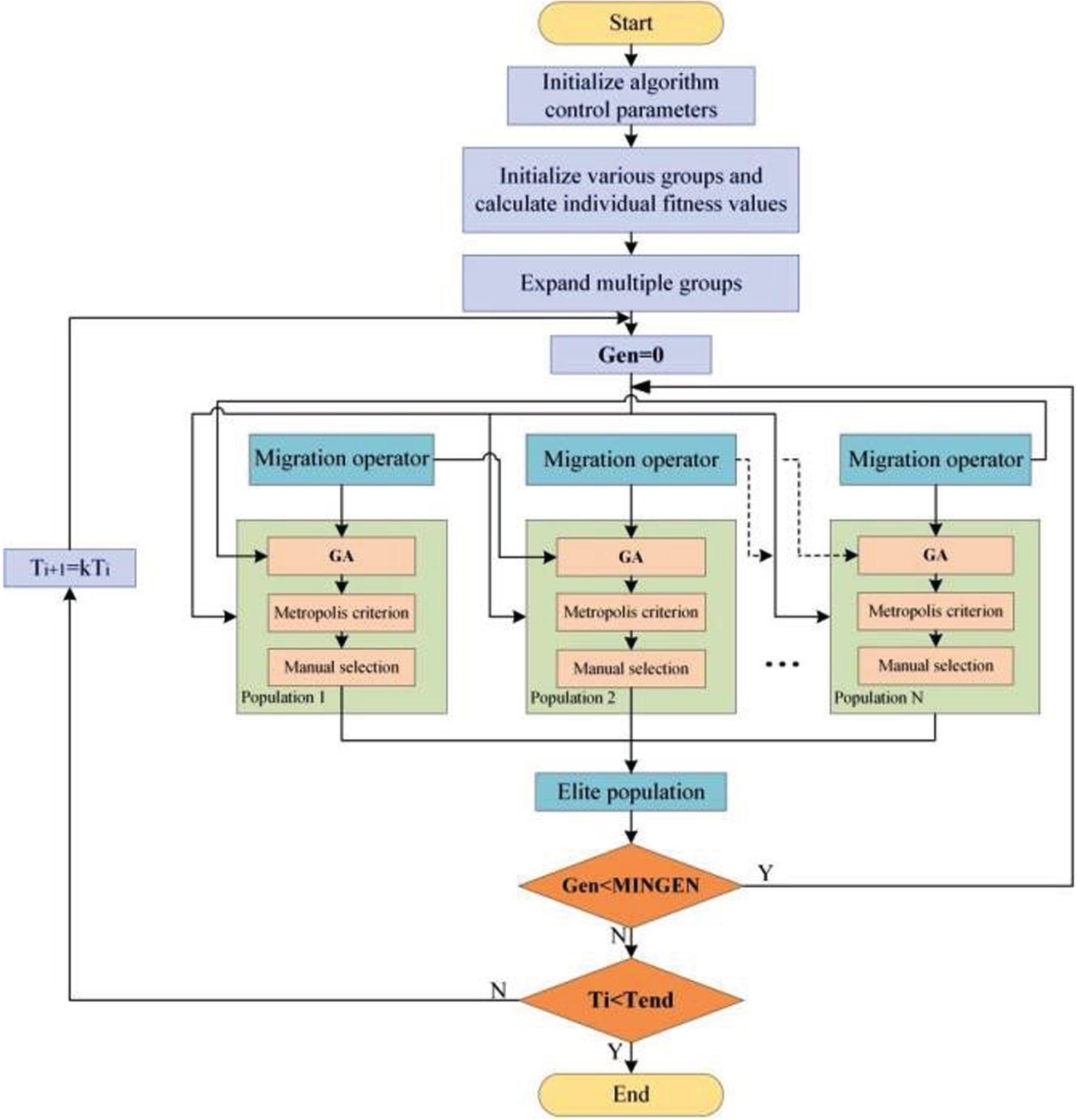
Design flowchart for SAMPGA.

Specific steps of the SAMPGA algorithm are shown below:

Step 1: Initialize each controller parameter of the algorithm: the number of populations denoted as M_p, the number of individuals in the population as NIND, and the number of generations of optimal individuals maintenance in the elite population as MINGEN. The same probability of generation gap for each population is set as P_n, the crossover probability as for each population, a random number in the interval [0.7 0.9], and the variation probability as P_m (i) , i ∈ [1M_p] for each population, a random number in the interval [0.001 0.05]. There are other parameters, including the initial annealing temperature T₀, temperature cooling factor k, and termination temperature T_end.

Step 2: Randomly generate NIND individuals for each population within the boundary as the initial populations and find the corresponding individuals’ fitness values.

Step 3: Expand multiple populations to start co-evolution and set the evolutionary generation count variable Gen = 0.

Step 4: Multiple populations collaborate in genetic operations such as selection, crossover and mutation, after which the fitness values of the old and new individuals are compared. When the fitness value of the new individual is greater than its old counterpart, the new individual replaces the old. Conversely, the new or old individual is selected according to the probability provided by the Metropolis criterion. At the same time, the migration operator periodically introduces the best individual from one population to another population during the evolutionary process, thus acting as a link among various populations.

Step 5: Save and move the best individuals in various populations to the elite population; when the best individuals in the elite population keep the number of generations less than MINGEN, then gen = gen+1, and turn to step 4; If not, turn to step 6.

Step 6: When T_i < T_end is satisfied, the algorithm ends and the global optimal solution is found. Otherwise, the cooling operation T_i = kT_i is implemented and the process moves to step 3.

3.2.2 SAMPGA algorithm’s performance tests

Five different test functions are used to evaluate the performance of the SAMPGA hybrid algorithm, and its results are then compared to those of the three other algorithms: GA, Simulated Annealing and Genetic Algorithm (SAGA), and MPGA.

(1) Test functions

➀ F1 (Binary function) $min f (x_{1}, x_{2}) = {x_{1}}^{2} + {x_{2}}^{2} x_{1}, x_{2} \in [- 100, 100]$ (24)

The F1 function is a two-dimensional single-peaked function that is able to find a theoretical global minimum of 0 at (0,0). The accuracy of the acceptable solution is 1.0×10^–6.

➁ F2 (Schaffer function) $\begin{matrix} min f (x_{1}, x_{2}) = 0.5 - \frac{{(\sin \sqrt{{x_{1}}^{2} + {x_{2}}^{2}})}^{2} - 0.5}{{[1 + 0.001 ({x_{1}}^{2} + {x_{2}}^{2})]}^{2}} \\ x_{1}, x_{2} \in [- 100, 100] \end{matrix}$ (25)

The F2 function is a two-dimensional multi-peaked function with multiple local minima and a theoretical global minimum of 0 at (0, 0), which is difficult to find because of the strong oscillatory nature of the function. The accuracy of the acceptable solution is 1.0×10^–2.

➂ F3 (Griewank function) $\begin{matrix} min f (x_{i}) = \sum_{i = 1}^{N} \frac{{x_{i}}^{2}}{4000} - \prod_{i = 1}^{N} cos (\frac{x_{i}}{\sqrt{i}}) + 1 \\ x_{i} \in [- 600, 600] (i = 1, \dots, N) \end{matrix}$ (26)

The F3 function is an N-dimensional non-linear multimodal function, the number of local minima is related to the dimensionality of the function, and the theoretical global minimum value of 0 can be obtained at . This test N is taken as 10, the accuracy of the acceptable solution is 1.0×10^–1.

➃ F4 (Ackley function) $\begin{matrix} min f (x_{i}) = - 20 exp (- 0.2 \sqrt{\frac{1}{n} \sum_{i = 1}^{N} {x_{i}}^{2}}) \\ - exp [\frac{1}{n} \sum_{i = 1}^{N} cos (2 π x_{i})] + 20 + e \\ x_{i} \in [- 100, 100] (i = 1, \dots, N) \end{matrix}$ (27) The F4 function is an N-dimensional multi-peaked function with a high number of local minima, and a theoretical global minimum value of 0 can be obtained at . This test N is taken as 10, the accuracy of the acceptable solution is 1.0×10^–2.

➄ F5 (Rosenbrock function) $\begin{matrix} min f (x_{i}) = \sum_{i = 1}^{N - 1} [100 {({x_{i}}^{2} - x_{i + 1})}^{2} + {(x_{i} - 1)}^{2}] \\ x_{i} \in [- 100, 100] (i = 1, \dots, N) \end{matrix}$ (28)

F5 function global minima are located in a smooth and narrow parabolic-shaped valley, the algorithm is difficult to identify the direction of the search for the optimal value based on the valid information provided by the function, the function can achieve a theoretical global minimum value of 0 at . This test N is taken as 10, the accuracy of the acceptable solution is 1.0×10^–2.

(2) Testing and comparison of the algorithms’ performance

Binary coding is adopted in this test because of its many advantages, such as simplicity, computer processing convenience, high coding accuracy and compliance with the minimum character set operation criterion. The number of bits in the binary code for each variable is set at 20, and the selection operator adopts random traversal sampling. The crossover mode is two-point crossover and the variation mode is binary variation.

The setting of the controller parameters significantly influences the performance improvement of the algorithm concerning globalization, convergence and stability. According to experience and testing requirements, uniform setting of the controller parameters for each algorithm are listed in Table 1.

Table 1

Table of algorithm control parameters

Algorithm Name	T₀	k	T_end	M_p	NIND	MINGEN	P _n	P _c	P _m
GA	-	-	-	-	30	10	0.95	0.7	0.01
SAGA	100	0.8	1	-	30	10	0.95	0.7	0.01
MPGA	-	-	-	10	30	10	0.95	[0.7 0.9]	[0.001 0.05]
SAMPGA	100	0.8	1	10	30	10	0.95	[0.7 0.9]	[0.001 0.05]

The proportion of optimal solutions that are found, average value of the objective function, average number of convergence generations that ensures an acceptable accuracy, and average running time of the algorithm are used as indicators of the algorithms’ performance when evaluating the advantages and disadvantages of each algorithm using the test functions. Each algorithm was tested with 50 trials using 5 test functions, and statistical results of the optimal objective function values for each test are shown in Table 2. Bolded numbers represent the optimal values in the four algorithm tests, and “-” indicates that the algorithm fails to achieve the accuracy of acceptable solutions on that test function.

Table 2

Comparison of algorithm test results

Algorithm	GA	SAGA	MPGA	SAMPGA
Find the optimal	F1	92	100	100	100
solution ratio (%)	F2	28	28	70	88
	F3	0	58	46	66
	F4	0	84	66	100
	F5	0	8	100	100
Average objective	F1	2.5925×10^–5	1.8190×10^–8	1.8190×10^–8	1.8190×10^–8
function	F2	0.0692	0.0484	0.0082	0.0047
	F3	0.4440	0.1090	0.1290	0.0982
	F4	7.0641	0.1474	0.3273	4.4282×10^–4
	F5	28.0834	18.1328	2.8211×10^–4	1.0950×10^–6
Standard deviation	F1	1.2268×10^–4	1.6712×10^–23	1.6712×10^–23	1.6712×10^–23
of the objective	F2	0.0822	0.0565	0.0088	0.0062
function	F3	0.2229	0.0745	0.0904	0.0672
	F4	7.7892	0.4446	0.6710	3.5399×10^–4
	F5	26.2160	22.9490	5.1898×10^–4	1.6176×10^–6
Average convergence	F1	97.22	316.74	38.62	257.16
algebra	F2	67.86	289.50	29.97	257.27
	F3	-	849.31	311.83	618.97
	F4	-	1145.26	418.24	735.52
	F5	-	2669.50	183.14	562.46
Average computing	F1	0.0261	0.0835	0.0956	0.6431
time (s)	F2	0.0156	0.0797	0.0739	0.6632
	F3	0.1456	0.6178	1.8281	3.6852
	F4	0.2021	0.8104	2.4124	4.3378
	F5	0.1923	3.9361	1.0335	3.2322

As shown in Table 2, conventional GA utilizes a single population for simple genetic operations such as selection, crossover and mutation. Although its running time is the shortest among the four algorithms, it tends to be trapped in the local optimal solutions, so the proportion of searching for optimal solutions is also the smallest. MPGA, on the other hand, extends the search interval by combining multiple populations for genetic evolution, which further improves the solution accuracy and efficiency of the algorithm. Its convergence generation is also the smallest. However, due to the lack of “annealing” operation, its accuracy of obtaining the optimal solution is lower than that of SAMPGA.

Both SAGA and SAMPGA accept inferior solutions with a certain probability during the evolution process to avoid premature convergence. Although such an operation enhances the accuracy of the solution and increases the probability of finding the global optimal solution, it extends the average operation time and slightly increases convergence generations, compared to other algorithms. In addition, SAMPGA not only speeds up the solution to a certain extent by using multiple swarm co-evolutions, but also searches for the largest proportion of optimal solutions among. Moreover, it has the smallest standard deviation of the objective function, which means that its solution fluctuation is small and the distribution is relatively concentrated.

Optimization results for each test function of the four algorithms are shown in Fig. 6. It can be observed that the horizontal coordinates represent the number of evolutionary generations and that the vertical coordinates suggest the value of the optimal individual objective function per generation. The number of evolutionary generations are uniformly set for the first 200 generations. In addition, SAMPGA always more accurately finds the global optimal solutions of the five test functions than other three algorithms, while efficiently avoiding local optimal solutions. To summarize, SAMPGA exhibits better stability and maintains a faster convergence rate in the evolution process.

Fig. 6

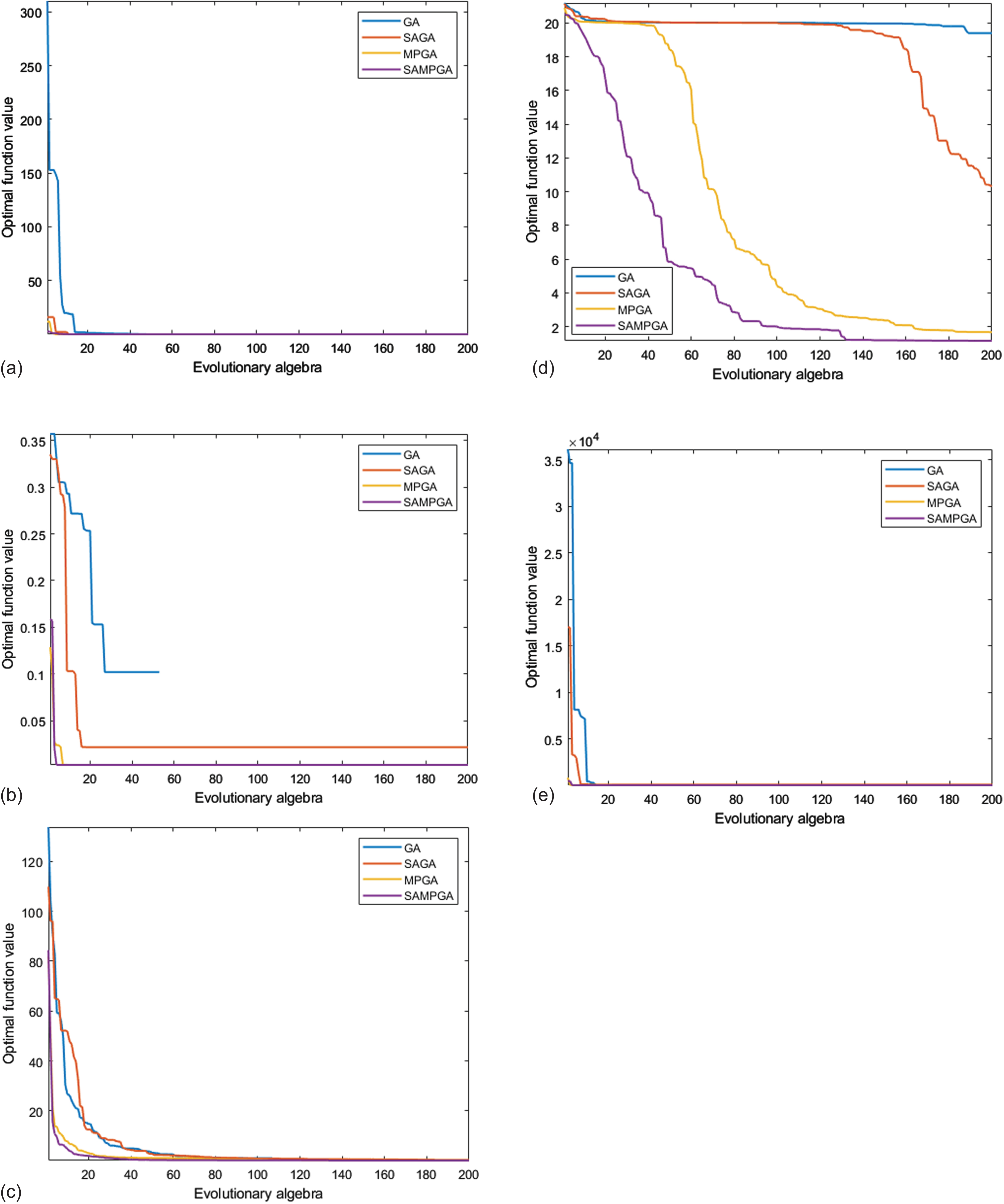
The evolutionary process of each algorithm under 5 test functions.

4 Soil parameters estimation and adaptation validation

In the spoil hopper deposition model, there are four parameters related to soil type, namely v_{s
_o}, k_e, β and ρ_s. These parameters constantly vary with changes in dredging location and soil type. Among them, β has been proved to exert little effect on spoil hopper sediment loading, so the empirical value 4 is taken here [16]. The ability to forecast the mass of the mud and sand fed into the TSHD and the mass of the water-mud combination overflow loss depends directly on the soil characteristics in the spoil hopper model. Therefore, soil parameters play a critical role in the process optimization of loading hopper.

4.1 Data acquisition and processing of the measured samples

The big TSHD “New Haihu 8” made seven vessel visits during routine dredging and loading operations in the Yangtze Estuary and Xiamen Port in China, and this information was collected to estimate soil parameters in this paper. The dredged soils contain fine-grained sands and medium sands respectively. For each vessel, 100 sets of data samples with a sampling interval of 30 seconds were selected, and each set included eight dimensions: overflow weir position, spoil hopper loading height, inlet flow and density of left and right suction pipe, spoil hopper capacity and spoil hopper loading mass. A sample of data for a particular vessel at Yangtze Estuary is shown in Table 3.

Table 3
Example of sample data from Yangtze Estuary

Serial number Overflow weir location (m) Hopper loading height (m) Left suction pipe inlet flow (m³/s) Right suction pipe inlet flow (m³/s) Left suction pipe inlet density (kg/m³) Right suction pipe inlet density (kg/m³) Hopper compartment capacity (m³) Hopper loading mass (t)

1 15.45 6.90 5.71 6.51 1.10 1.14 6577.27 6074.55

2 15.45 7.20 5.71 6.46 1.11 1.13 6977.34 6424.31

3 15.45 7.48 5.70 6.47 1.14 1.14 7355.62 6812.66

4 15.45 7.62 5.68 6.44 1.15 1.15 7545.58 7108.93

5 15.45 7.95 5.65 6.45 1.16 1.14 7977.62 7562.86

… … … … … … … … …

Serial number	Overflow weir location (m)	Hopper loading height (m)	Left suction pipe inlet flow (m³/s)	Right suction pipe inlet flow (m³/s)	Left suction pipe inlet density (kg/m³)	Right suction pipe inlet density (kg/m³)	Hopper compartment capacity (m³)	Hopper loading mass (t)
1	15.45	6.90	5.71	6.51	1.10	1.14	6577.27	6074.55
2	15.45	7.20	5.71	6.46	1.11	1.13	6977.34	6424.31
3	15.45	7.48	5.70	6.47	1.14	1.14	7355.62	6812.66
4	15.45	7.62	5.68	6.44	1.15	1.15	7545.58	7108.93
5	15.45	7.95	5.65	6.45	1.16	1.14	7977.62	7562.86
…	…	…	…	…	…	…	…	…

Real-time data collected might have been disturbed by external factors, resulting in noisy data. Therefore, it’s important to first denoise the data we collected. Compared with traditional time-domain filtering and frequency domain filtering methods, wavelet transform denoising ensures effective noise filtering while retaining the maximum amount of detailed local information of the original data, so we adopted the wavelet soft thresholding method to filter noisy data [29]. Figure 7 shows the comparative results before and after wavelet denoising on partial measured data (left suction pipe inlet flow and density).

Fig. 7

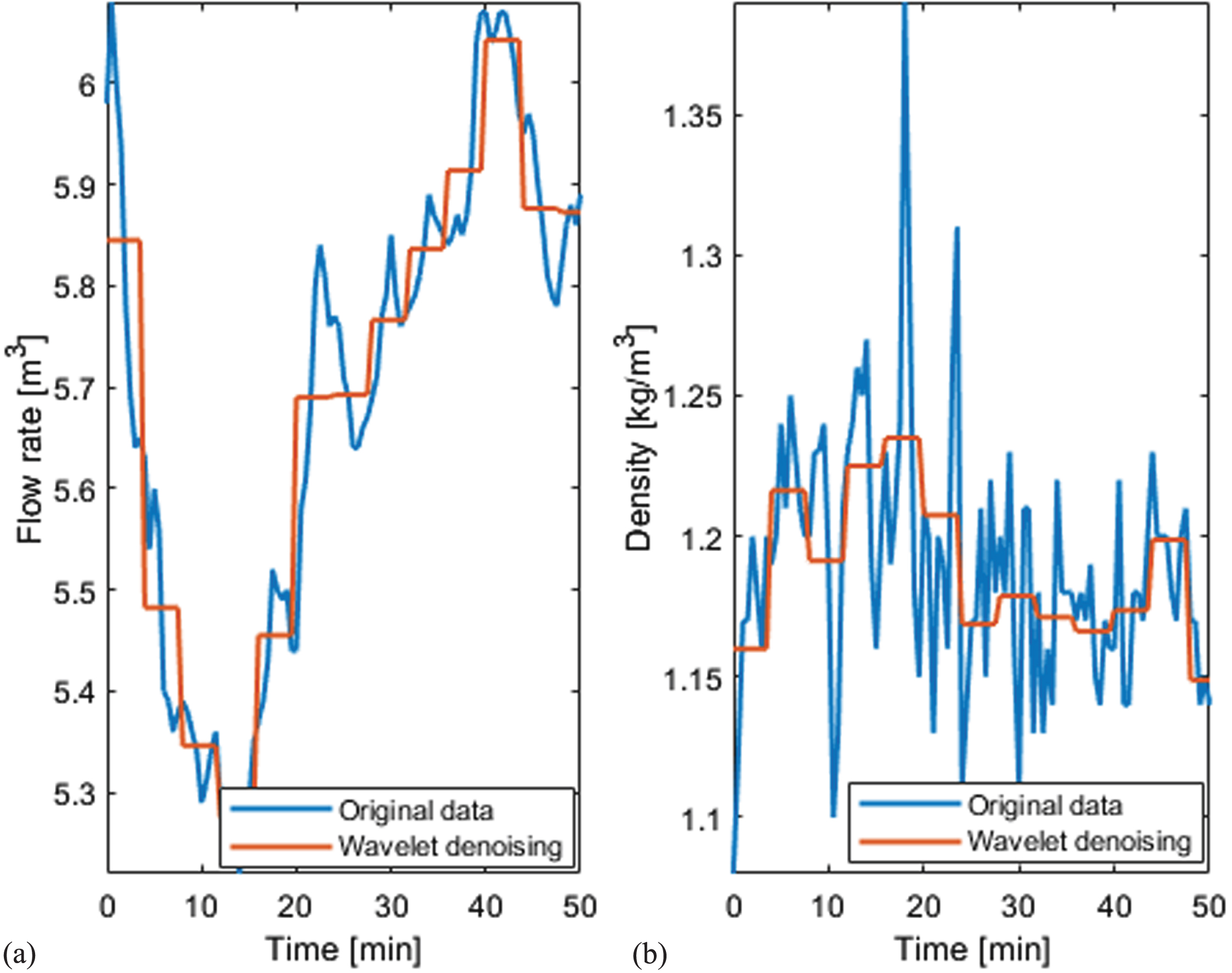
Comparison of partial measured data before and after wavelet transform denoising.

4.2 Soil parameters estimation

To test the effectiveness of the SAMPGA algorithm in estimating soil parameters in the spoil hopper sedimentation model, three pre-estimated soil parameters were selected and a range of values was assigned to them: v_so ∈ [0.0010 . 4] m/s, k_e ∈ [0.130] and ρ_s ∈ [13002300] kg/m³. The results of SAMPGA were compared with that of the other three algorithms.

4.2.1 Setting of algorithm coding bits, fitness function and controller parameters

(1) Determining of the number of bits to be coded

The number of bits for individual chromosome binary coding should be determined before estimating the soil parameters. Since the spoil hopper sedimentation model contains 3 pre-estimated soil parameters, v_{s
_o}, k_e and ρ_s, to improve the accuracy of chromosome coding, 20-bit binary numbers were used in each parameter variable coding. Then the length of each individual chromosome is represented by a binary code string of 20×3. The selection operator still used random traversal sampling, and the crossover operator and variation operator were two-point crossover and binary variation, respectively.

(2) Creating the fitness function

The fitness function measures the individuals’ strengths and weaknesses. Each individual’s objective function and fitness function are expressed in the form of equations (29) and (30). $J (θ) = \sqrt{\frac{\sum_{i = 1}^{N} {(\overset{\land}{y} (i, θ) - y (i))}^{2}}{M}}$ (29)

Where i is the time point when the sample data was collected, θ is the pre-estimated soil parameter, M is the total number of collected sample data $\overset{\land}{y} (i, θ)$ and y (i) represent the model output and measured values of the loaded mass at a given moment. A smaller J (θ) suggests a higher accuracy of the soil parameter estimation.

The fitness function is the inverse of the objective function and its expression is: $Fin (θ) = \frac{1}{J (θ)}$ (30)

(3) Setting of the controller parameters

According to several experimental tests, the ultimate settings of the controller parameters are listed in Table 4.

Table 4

Setting parameters of optimization algorithm

Algorithm Name	T₀	k	T_end	M_p	NIND	MINGEN	P _n	P _c	P _m
GA	-	-	-	-	30	3	0.95	0.7	0.01
SAGA	100	0.8	1	-	30	3	0.95	0.7	0.01
MPGA	-	-	-	5	30	3	0.95	[0.7 0.9]	[0.001 0.05]
SAMPGA	100	0.8	1	5	30	3	0.95	[0.7 0.9]	[0.001 0.05]

4.2.2 Analysis and comparison of algorithm optimization results

The loading operation data in Yangtze Estuary of the “New Haihu 8” TSHD (in this study, the 4th trip data) is randomly selected as the dataset. Then GA, SAGA, MPGA and SAMPGA are applied to estimate the soil parameters of the spoil hopper sedimentation model for 50 times. Changes in the objective function value of the optimal individual in each generation during a certain evolution are shown in Fig. 8. The number of evolutionary generations is chosen from 1 to 50, as represented by the horizontal coordinate. The objective function value of the optimal individual at each generation is represented by the vertical coordinate.

Fig. 8

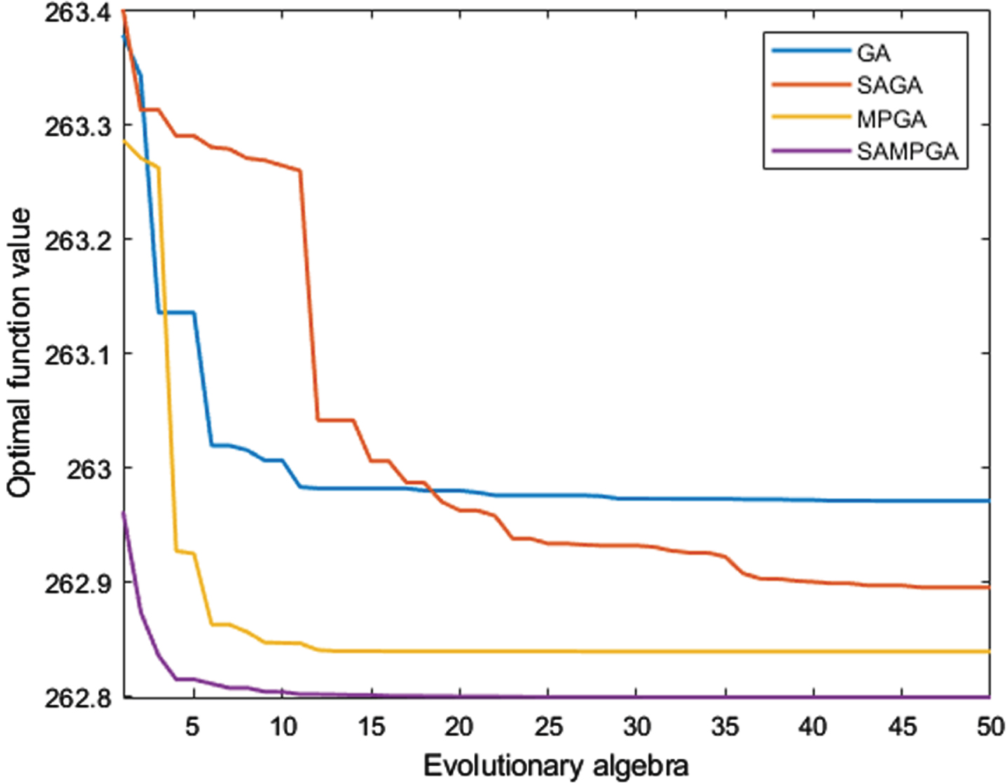
Evolutionary process for each algorithm.

As can be seen from Fig. 8, compared with the evolutionary process of GA, SAGA and MPGA, SAMPGA maintains a lower objective function value from the initial generation and its optimal objective function value is the smallest. It has converged to the overall optimal solution around the 12th generation of evolution with the fastest convergence speed. In contrast, GA and SAGA have not fully converged until the 50th generation.

To obtain a clearer and more intuitive understanding and comparison of the performance indicators of each algorithm during the 50 soil parameters estimations, the optimal results obtained by the algorithms for each operation are now counted as follows. Bolded numbers represent the optimal values among the four algorithms.

As shown in Table 5, in comparison to other algorithms, SAMPGA has the smallest average objective function value, minimum objective function value and standard deviation of the objective function. Its estimated soil parameters are v_{s
_o} = 0.096587 m/s, k_e = 25, and ρ_s = 1375 kg/m³, suggesting that SAMPGA significantly improves the accuracy of soil parameters estimation after the annealing operation and the co-evolution of multiple groups are introduced and that the distribution of the objective function values is more concentrated. In addition, since SAGA, MPGA and SAMPGA obtained almost the same optimal objective function value in each estimation within the total 50 soil parameters estimations, resulting in equal mean and minimum values of the corresponding objective functions attained by the algorithms. This result also shows that the performance of the algorithms is stable and hasn’t been easily influenced by external factors. Specifically, SAGA uses the Metropolis criterion for focused sampling to avoid falling into a local optimum, which leads to a much higher probability of accepting inferior solutions and thus the largest number of convergence generations. Compared with SAGA, although SAMPGA performs the same sampling operation, it performs the genetic operation on multiple populations simultaneously and the convergence speed has accelerated. The operation performed by GA is simpler and less time is spent on computation, while MPGA and SAMPGA performed complex multiple population genetic operations with relatively long computation time.

Table 5

Comparison of soil parameters estimation results

Algorithm	Average objective	Objective function	Objective function	Average	Average
Name	function	Maximum value	Standard deviation	Convergence algebra	Operation time(s)
GA	262.9913	262.9715	0.0717	76.6	0.1353
SAGA	262.8923	262.8923	4.3470×10^–11	207.24	0.3222
MPGA	262.8387	262.8387	1.3216×10^–5	63.16	0.4053
SAMPGA	262.7987	262.7987	5.7421×10^–14	151.48	0.9246

In summary, although the average running time of SAMPGA was slightly longer, it achieved higher accuracy, concentrated solution distribution and relatively faster convergence than other algorithms. It effectively overcomes the “premature” phenomenon that may occur in GA and MPGA. Meanwhile, SAMPGA is more suitable for offline soil parameter estimation in spoil hopper deposition models without time constraints. For scenarios with higher real-time requirements, MPGA, which is slightly less accurate than SAMPGA, can also be used for online soil parameter estimation.

To further verify the accuracy of SAMPGA in soil parameters estimation, the estimated soil parameters are now used in the spoil hopper deposition model to predict the loaded mass of the model output. Comparison between the estimated outcomes and the measured loading mass data from the 4th vessel were conducted, as shown in Fig. 9.

As shown in Fig. 9(a), when the TSHD started loading, the model output and the measured values of the loading mass increased rapidly with time passing. 20 minutes later, because of the low-density mixture flowing out from the overflow weir, the loading mass increased slowly until the loading operation stops at the 50th minute. The model output values and measured values in Fig. 9(a) indicate a relatively better fit. Figure 9(b) displays the error distribution of the model output values of the loading mass relative to the measured values. It can be observed that the interval range of the relative error distributions of the model output and measured values of the loading mass is small and the error distribution of the loading mass for most sample data centers around the range of [-0.02 0.02], which further indicates the relatively high accuracy of the estimated parameters by SAMPGA.

Fig. 9

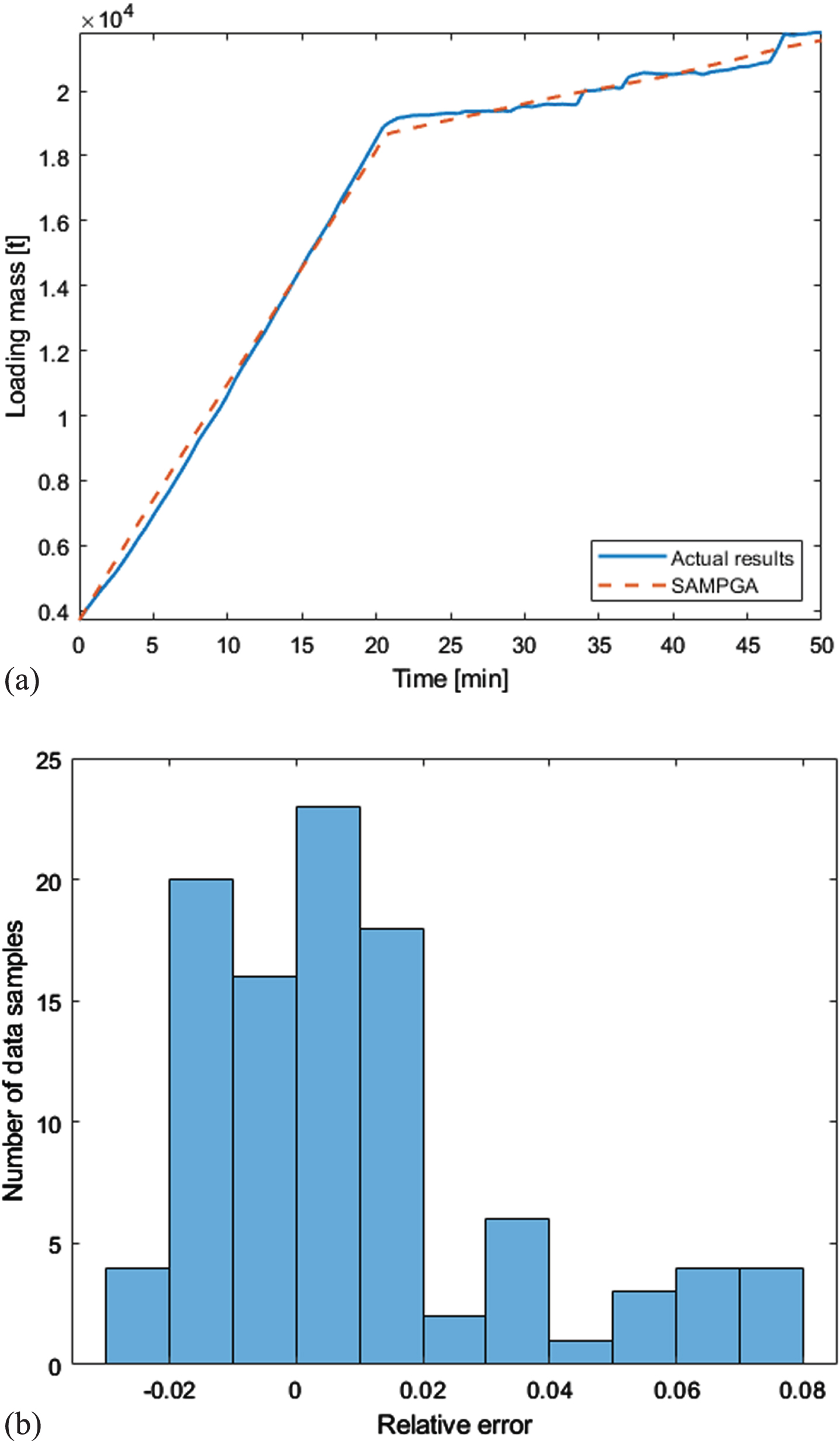
Comparison of loading spoil hopper mass model output with actual measurement results.

4.2.3 Calculation of overflow density, sand bed height and ton of dry solids

Like the case in soil parameter estimations, the overflow density and sand bed height cannot be directly measured by measuring instruments as well. As inspired by the 4th operating data of the “New Haihu 8” TSHD, an indirect prediction of the overflow density and sand bed height can be realized by substituting the soil parameters of the spoil hopper deposition model, as shown in Fig. 10.

In Fig. 10(a) it can be seen that the inlet density was consistently greater than the overflow density. At around 20 minutes, the overflow phase started, and the lower density mud-water mixture above the spoil hopper flowed out from the overflow weir. The overflow density fluctuated in a small range in the subsequent time, and its maximum value was 1.0481×10³ kg/m³. In Fig. 10(b), the height of the overflow weir was always the same, 15.45 m. The level of the spoil hopper rose continuously with the loading operation of the TSHD and reached the overflow weir height about 20 minutes later and then remained unchanged. The sand bed height increased with the loading process progression and finally stopped when the sand bed height approached the overflow weir height. At this time, the height of the sand bed reached 14.6189 m.

Fig. 10

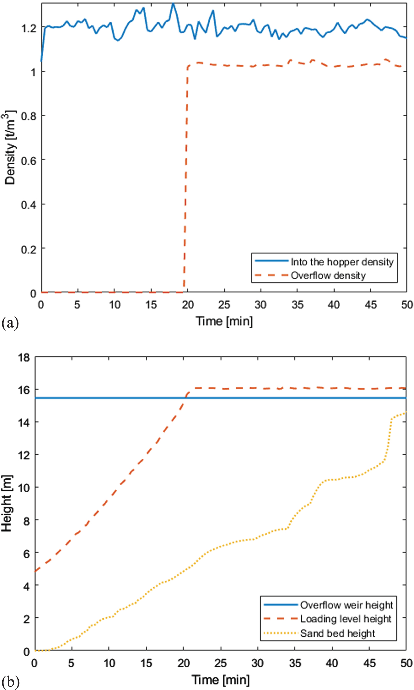
Overflow density and sand bed height during loading.

An important index for the assessment of the loading performance of the TSHD is the ton of dry solids (TDS), whose expression is equation (31). It reflects the mass of dry mud and sand loaded in the spoil hopper except for pure water during the loading process of the dredger. At the same time, it is also closely related to the mass of overflow loss, as shown in Fig. 11. The overflow mass m_o will directly affect the final loading yield and efficiency of the TSHD, so it needs to be focused on during the loading operation of the dredger, and its expression is equation (32).

Fig. 11

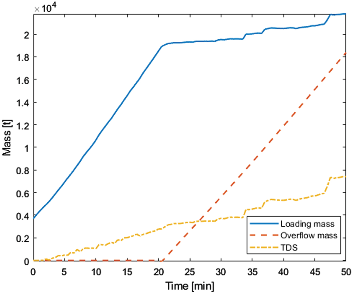
Loading mass, TDS and overflow mass.

$TDS = \frac{(m_{t} - V_{t} ρ_{w}) ρ_{q}}{ρ_{q} - ρ_{w}}$ (31)

Where V_t and m_t represent the volume and mass of the mixture in the spoil hopper respectively; where ρ_w and ρ_q represent the water density and quartz density respectively. $d m_{o} = Q_{o} ρ_{o} dt$ (32)

Where Q_o and ρ_o denote the overflow flow rate and overflow density of the mixture, respectively.

From Fig. 11, it can be seen that the loading mass and TDS increased rapidly at the beginning of the loading operation. In the 20th minute, the overflow occurred. The loading mass and TDS curves showed a significant bend, indicating a slowdown in their rate of increase. Meanwhile, the overflow losses began to appear and the overflow mass increased linearly during the subsequent dredger loading operation. Because the dredged soils in the Yangtze Estuary were so fine-grained that the sediment particles couldn’t properly settle down in the spoil hopper, causing too many fine-grained particles to flow out of the spoil hopper through the overflow weir. In the 50th minute, the loading ended and the overflow losses reached 1.8382×10⁴t, while the total loading mass of the hopper was 2.1794×10⁴t, indicating that a large overflow loss existed during the 4th loading operation of the TSHD. In addition, an excessive overflow loss reduced the weight of dry soils in the spoil hopper, which was 7.0486×10³t when the loading ended. This required immediate adjustment of the TSHD loading system control strategy and equipment parameters to reduce the overflow losses in other loading operation periods, so as to improve the dredger loading yield and efficiency.

4.3 Validation of soil parameters adaptation

In order to investigate the adaptability of the soil parameters under other vessel trips at the same and different dredging areas, the estimated parameters obtained from the 4th vessel trip at Yangtze Estuary could be substituted into the sedimentation model. Combining the data from Yangtze Estuary and other vessel trips in the Xiamen Port, the degree of fit between the output values of the loading mass model and the measured values was checked to test whether the fixed soil parameters can still be applied to other vessel trips in the same and different dredging areas. Meanwhile, the variance assessment factor (VAF) was applied to evaluate the model’s performance, and the outcomes of the soil parameter fitness assessment are shown in Table 6. VAF calculates the weighting of the residual variance (var(y)) of the variance of the measured values y, and the larger the value, the smaller the error between the model output value and the measured value. Since VAF is less sensitive to data noise, VAF was used in model evaluation, and its expression is:

Table 6
Soil parameter suitability studies

Dredging area Yangtze Estuary Xiamen Port

Evaluation J VAF J VAF

indicators

Number of vessels 1 771.7619 0.9475 2002.1827 0.8552

2 910.1531 0.9740 1544.4715 0.9482

3 662.4872 0.9771 1832.1883 0.9615

4 262.7987 0.9977 1483.7693 0.9794

5 574.8783 0.9879 1139.5660 0.9763

6 594.6721 0.9882 928.3890 0.8879

7 702.9937 0.9658 2414.5429 0.9547

Average 639.9636 0.9769 1620.7300 0.9376

Dredging area	Yangtze Estuary	Xiamen Port
Number of vessels	1	771.7619	0.9475	2002.1827	0.8552
	2	910.1531	0.9740	1544.4715	0.9482
	3	662.4872	0.9771	1832.1883	0.9615
	4	262.7987	0.9977	1483.7693	0.9794
	5	574.8783	0.9879	1139.5660	0.9763
	6	594.6721	0.9882	928.3890	0.8879
	7	702.9937	0.9658	2414.5429	0.9547
Average		639.9636	0.9769	1620.7300	0.9376

$VAF = 1 - \frac{var (y - \hat{y})}{var (y)}$ (33)

Where y and $\hat{y}$ are the measured value and model output value respectively.

As shown in Table 6, fixed soil parameter estimation exhibits good adaptability under different vessel trips in the same dredging area. While the J values obtained from other vessel trips in the Yangtze Estuary are slightly larger compared to the four, VAF always remains a higher value, indicating that there is a small error between the model output loading mass and the measured values. In contrast, the mean values of J under other vessel trips in different dredging areas are larger and the mean values of VAF are smaller, indicating that changes in dredging areas make the soil parameters less adaptable and that re-estimation of soil parameters in the spoil hopper deposition model is required.

5 Conclusion

SAMPGA proposed in this paper, which combines SA with strong local search ability and MPGA with strong global search ability, and introduces both annealing and various swarm genetic operations, is applied to the estimation of soil parameters in the spoil hopper sedimentation model. The experimental results suggest that SAMPGA has the fastest convergence speed and the highest solution accuracy in soil parameter estimation, among four algorithms (SAMPGA, GA, SAGA and MPGA).

To verify the validity of the soil parameters estimation, the model output values of the loading mass were analyzed and compared with the measured values. The results indicated a high degree of fit and a small error between the two sets of values, suggesting that the estimated soil parameters values have a high degree of accuracy.

Tests combined with real ship data showed that the soil parameters well adapted to the loading in different vessel trips at the same dredging area, which can be applied to the spoil hopper deposition model to identify important variables such as overflow density, sand bed mass and height.

Using real shipping data from the Xiamen Port, the estimated soil parameters of the Yangtze Estuary were used in the spoil hopper sedimentation model. In addition, the output values of the loading mass model were obtained which showed large errors compared with the actual measured values at Xiamen Port. This indicates that the soil parameters have lowered adaptability in different dredging areas, and that the soil parameters in the spoil hopper model need to be re-estimated.

The research results concerning the spoil hopper model and the methods of soil parameters estimation in this paper offer insightful suggestions and inspirations for the smooth development of the loading hopper optimization research.

The predictive accuracy of the productivity prediction model in the example of this paper needs to be improved, but the dredging operation of the TSHD is carried out under different soil quality, hydrology, meteorological sea state and soil treatment conditions, and there are too many unpredictable factors affecting productivity, and productivity fluctuates frequently with no obvious regularity, and the prediction error is within the acceptable range relative to the complexity of the simulation problem, and the modeling of the TSHD has a certain significance in guiding construction. If the soil quality in the mud extraction area is homogeneous, the terrain is relatively flat, the sample distribution is more uniform, and more information such as the opening degree of the drinking window of the rake head can be collected, the prediction accuracy of the prediction model will be improved to a great extent.

Footnotes

Acknowledgments

This work was supported by the China Ministry of Industry and Information Technology High Technology Ship Project [Document No. [2019]360].

Consent for publication

All authors reviewed the results, approved the final version of the manuscript and agreed to publish it.

Data availability

The experimental data used to support the findings of this study are available from the corresponding author upon request.

Conflicts of interest

The authors declared that they have no conflicts of interest regarding this work.

References

Bai

, Li

, Song

, Ren

, Qin

and Fu

, Productivity analysis of trailing suction hopper dredgers using stacking strategy, Automat Constr 122 (2021). https://doi.org/10.1016/j.autcon.2020.103470.

Camp

, A study of the rational design of settling tanks, Sewage Works J 8 (1936), 742–758.

Yagi

, Sedimentation effects of soil in hopper, World Dredging Conference III 1970.

Vlasblom

and Miedema

, A theory for determining sedimentation and overflow losses in hoppers, World Dredging Conference XIV 1995.

Miedema

and Vlasblom

, Theory for hopper sedimentation, TAMU WEDA Conference 1996.

Ooijens

, Adding dynamics to the camp model for the calculation of overflow losses, Terra Et Aqua 76 (1999), 12–21.

Ooijens

, Gruijter

, Nieuwenhuijzen

and Vandycke

, Research on hopper settlement using large-scale modeling, In Proceedings of the CEDA Dredging Days 2001 (2001).

Rhee

, Numerical simulation of the sedimentation process in a trailing suction hopper dredge, WO-DCON XVI 2001.

Rhee

, Modelling the sedimentation process in a trailing suction hopper dredger, Terra Et Aqua 86 (2002), 18–27.

10.

Rhee

, On the sedimentation process in a trailing suction hopper dredger. Doctoral thesis, Delft University of Technology, South Holland Province, 2002.

11.

Braaksma

, Babuska

and Klaassens

, A computationally efficient model for predicting overflow mixture density in a hopper dredger, Terra Et Aqua 106 (2007), 10–28.

12.

Miedema

, The effect of the bed rise velocity on the sedimentation process in hopper dredges, World Dredging Conference XIX 10 (2010), 10–31.

13.

Hao

, Hong

and Wang

, Simulation of deposition and scour of non-cohesive sediment in full loading process of TSHD, Port Waterway Eng 12 (2012), 119–125. https://doi.org/10.16233/j.cnki.issn1002-4972.2012.12.043.

14.

Decrop

, De

, Toorman

and Sas

, A parameter model for dredge plume sediment source terms, Ocean Dynam 67 (2017), 137–146. https://doi.org/10.1007/s10236-016-1017-0.

15.

Chen

, He

, Xiong

, Li

and Liu

, Study on the dynamic characteristics of the overflow advection and diffusion of trailing suction hopper dredgers based on CFD, Ocean Eng (2022), 252. https://doi.org/10.1016/j.oceaneng.2022.111263.

16.

Braaksma

, Model-based control of hopper dredgers. Doctoral thesis, Delft University of Technology, South Holland Province, 2008.

17.

, Yuan

, Lecture notes in electrical engineering, Springer Verlag: Berlin, Germany, (2016), 811–815.

18.

Stano

P.M.

, Tilton

A.K.

and Babuska

, Estimation of the soil-dependent time-varying parameters of the hopper sedimentation model: The FPF versus the BPF, Control Eng Pract 24 (2014), 67–78. https://doi.org/10.1016/j.conengprac.2013.11.005.

19.

Stano

P.M.

, Nonlinear state and parameter estimation for hopper dredgers. Doctoral thesis, Delft University of Technology. South Holland Province, 2013.

20.

Stano

, Lendek

, Braaksma

, Babuska

, de Keizer

and den Dekker

A.J.

, Parametric bayesian filters for nonlinear stochastic dynamical systems: a survey, IEEE T Cybernetics 43 (2013), 1607–1624. https://doi.org/10.1109/TSMCC.2012.2230254.

21.

, Zhang

, Yao

, Zhu

and Fu

, Mathematic modeling and CFD simulation of the sedimentation process in a TSHD, Mar Georesour Geotec, 2022. https://doi.org/10.1080/1064119X.2022.2059421.

22.

Sape

, Introduction dredging engineering: oe4607. Delft University of Technology Press: Delft, Netherlands, (2015), 215–262.

23.

Mafarja

and Mirjalili

, Hybrid whale optimization algorithm with simulated annealing for feature selections, Neurocomputing 260 (2017), 302–312. https://doi.org/10.1016/j.neucom.2017.04.053.

24.

Shi

, Long

, Li

and Deng

, Multi-population genetic algorithm with ER network for solving flexible job shop scheduling problems, Plos One (2020), 15. https://doi.org/10.1371/journal.pone.0233759.

25.

Shishido

H.Y.

, Estrella

J.C.

, Motta Toledo

C.F.

and Arantes

M.S.

, Genetic-based algorithms applied to a workflow scheduling algorithm with security and deadline constraints in clouds, Computers & Electrical Engineering 69 (2018), 378–394. https://doi.org/1016/j.compeleceng.2017.12.004.

26.

, Zhao

, Huang

, Optimization methods and their MATLAB implementation. Beijing University of Aeronautics and Astronautics Press: Beijing, China, (2018), 199–208.

27.

Gholinezhad

and Torabi

, Research on multi-user air cargo route selection based on improved genetic algorithm, J Intell Fuzzy Syst 38 (2020), 39–46. https://doi.org/10.3233/JIFS-179378.

28.

, Wang

, Zhou

, Fan

and Xia

, Multi-swarm co-evolution based hybrid intelligent optimization for bi-objective multi-workflow scheduling in the cloud, IEEE T Parall Distr 33 (2022), 2183–2197. https://doi.org/10.1109/TPDS.2021.3122428.

29.

Zhang

, Zou

, Guo

and Yin

, Wavelet denoising method with a novel wavelet threshold function applied in enoising ship maneuvering test data, Indian J Geo-Mar Sci 46 (2017), 1780–1783.

Hybrid optimization algorithm for estimating soil parameters of spoil hopper deposition model for trailing suction hopper dredgers

Abstract

Keywords

1 Introduction

2 Loading process spoil hopper deposition model

3.1 Overview of SA and MPGA

3.1.1 Introduction of SA

3.2.1 SAMPGA algorithm design

4.1 Data acquisition and processing of the measured samples

4.2.1 Setting of algorithm coding bits, fitness function and controller parameters

Footnotes

Acknowledgments

Consent for publication

Data availability

Conflicts of interest

References