ISODF-ENN:Imbalanced data mixed sampling method based on improved diffusion model and ENN

Abstract

In the era of big data, the complexity of data is increasing. Problems such as data imbalance and class overlap pose challenges to traditional classifiers. Meanwhile, the importance of imbalanced data has become increasingly prominent, it is necessary to find appropriate methods to enhance classification performance of classifiers on such datasets. In response, this paper proposes a mixed sampling method (ISODF-ENN) based on iterative self-organizing (ISODATA) denoising diffusion algorithm and edited nearest neighbors (ENN) data cleaning algorithm. The algorithm first uses iterative self-organizing clustering algorithm to divide minority class into different sub-clusters, then it uses denoising diffusion algorithm to generate new minority class data for each sub-cluster, and finally it uses ENN algorithm to preprocess majority class data to remove the overlap with the minority class data. Each sub-cluster is oversampled according to sampling ratio, so that the oversampled minority class data also conforms to the distribution of original minority class data. Experimental results on keel datasets demonstrate that the proposed method outperforms other methods in terms of F-value and AUC, effectively addressing the issues of class imbalance and class overlap.

1 Introduction

Data imbalance has always been a prominent problem in machine learning. When a dataset contains significant differences in the number of instances among classes, it is considered an imbalanced dataset. Specifically, a class with a larger number of instances is referred to as majority class, while a class with a smaller number of instances is referred to as minority class [1]. Because we mainly focus on minority class data in imbalanced problems, the minority class is commonly referred to as positive class and labeled with class label 1, while the majority class is referred to as negative class and labeled with class label 0. Class imbalance is a common issue in various real-life applications, such as credit card fraud detection, network intrusion detection, disease diagnosis, and spam email filtering,etc [2–5]. The number of minority data in these fields is relatively small, but it is more worthy of study than majority class data. However, traditional classifiers such as support vector machine (SVM), decision tree (DT), and naive bayesian (NB) classifiers tend to focus on achieving the highest overall accuracy, so all data are treated equally [6]. Consequently, the accuracy of classification on majority class data is high and the accuracy of classification on minority class data is relatively low, which cannot handle imbalanced datasets effectively. As a result, traditional classifiers are not effective in handling imbalanced datasets [7].

In addition to data imbalance, the classification of imbalanced data is often affected by class overlap and data noise [8, 9]. Some studies found that in some datasets, class overlap has a more significant negative impact on classifiers than data imbalance [10, 11]. This poses a greater challenge to deal with imbalanced data. In order to effectively address the issue of imbalanced data classification, researchers have proposed numerous methods. We categorize these methods into two main groups: data-level and algorithm-level. Data-level methods involve altering the distribution of the original data to balance the sample quantities. Common data-level methods include undersampling, oversampling, and mixed sampling. Undersampling achieves balance by reducing the number of samples in the majority class. However, excessive removal of majority class samples can lead to the loss of its inherent data characteristics, thereby reducing classification accuracy. Oversampling achieves balance by increasing the number of samples in the minority class. But simple oversampling approaches can lead to overfitting and introduce noise. Mixed sampling combines these two methods to alleviate the drawbacks of individual approaches. Algorithm-level methods primarily focus on modifying the classification algorithm directly. They are mainly categorized into cost-sensitive learning and ensemble learning methods. Cost-sensitive learning takes into account the cost of misclassification of each data point. So misclassification of minority class data will be assigned a higher cost compared to majority class data. Ensemble learning methods make decisions by combining the votes of multiple weak classifiers. However, algorithm-level methods often have limitations that require appropriate cost matrices designed for the dataset, and ensemble learning typically needs to be used in conjunction with data-level methods.

In the past few decades, several algorithms have been proposed to effectively improve the performance of classifiers on imbalanced datasets. SMOTE (Synthetic Minority OverSampling Technique) [12] algorithm has become a popular oversampling method since its inception. The algorithm generates minority samples by linear interpolation instead of simple random replication, which alleviates the problem of overfitting and partially address the problem of imbalanced data. However, SMOTE treats all minority class instances equally, which can lead to noise generation and alterations to the data distribution, ultimately increasing the degree of sample overlap [13]. To address this issue, Borderline-SMOTE (B-SMO) [14] divides minority class into three categories (safe, danger, and noise), and only oversamples the instances classified as danger to distinguishe the boundary and non-boundary regions of the minority class. Xu proposed an oversampling algorithm combining SMOTE and k-means (KNSMOTE) [15]. KNSMOTE clusters the minority data through k-means, then calculates the safe samples in the sub-clusters, and synthesizes new data by linear interpolation of the safe samples Lin [16] proposed a clustering-based under-sampling method (KmUnder): this method clusters the data in the data preprocessing stage, add the step of clustering the data before under-sampling, and the number of clusters remains the same as the number of minority classes. The cluster center or the nearest neighbor of the cluster center is used as the sample of the majority class and merged with the minority class to obtain a balanced dataset. Tomek Links (TL) [17] and ENN [18] are widely used for data cleaning. TL improves the classification performance of classifiers by removing Tomek links, while ENN enhances it by eliminating misclassified majority class samples.

In recent years, there has been an increasing number of methods using deep learning to address the issue of imbalanced data. Among these, a representative approach involves the use of generative adversarial networks (GAN) [19] to generate synthetic samples that resemble the original distribution. Ding [20] proposes a method based on the combination of clustering and generative adversarial network(TWGAN-GP). This method undersamples the majority class data by clustering method, and then uses GAN to generate minority data to achieve a balanced dataset. But GAN usually suffer from problems such as gradient vanishing and mode collapse, and are not suitable for dealing with discrete forms of data. The denoising diffusion model generates samples by adding noise to original samples and learning the reverse diffusion process, which is operable and flexible. Based on this, this paper proposes a method combining the improved denoising diffusion algorithm based on clustering and ENN algorithm to solve imbalanced datasets. The main contributions of this study are as follows:

1. We propose an improved denoising diffusion model, which uses ISODATA to preprocess the data before synthesizing the data to improve the distribution of the synthetic data.

2. We propose an improved denoising diffusion model. The reverse process is trained through the BP neural network to improve the learning ability of the model for discrete data.

3. Solve the problem of data overlap in imbalan-ced data through the ENN algorithm.

2 Preliminary theory

2.1 Dynamic clustering

Clustering is an important method for data processing, and it is also commonly used in unsupervised learning [21]. Systematic clustering methods do not allow for those samples that were misclustered before to be re-clustered, while dynamic clustering methods enable samples to move from one class to another. The dynamic clustering method is one of the widely used methods, which consider two concepts: (1) incrementality of the learning methods to devise clustering methods and (2) self-adaptation of the learned model (parameters and structure) [22].

Dynamic clustering first selects the initial point to obtain initial clusters. Then in the classification process, class centers are repeatedly calculated to update the cluster until certain conditions are met, according to some regulations. The framework of this process is shown in Fig. 1.

Fig. 1

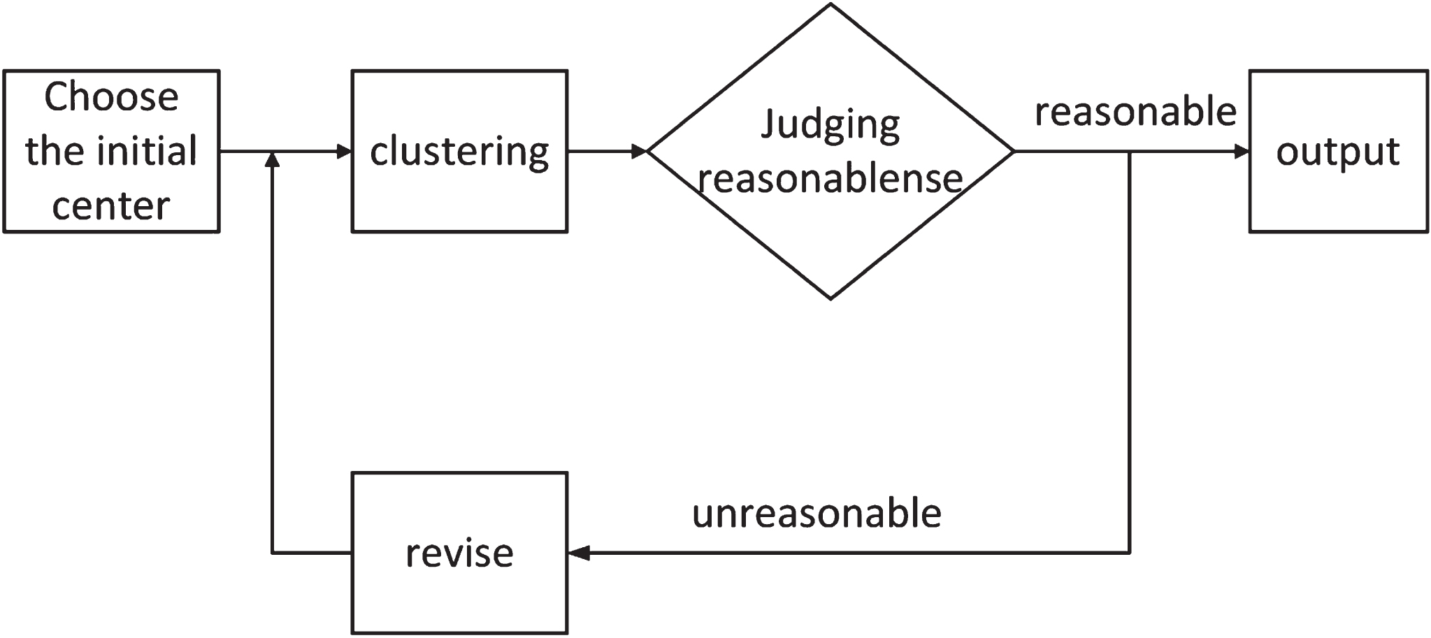
Basic process framework of dynamic clustering.

2.2 Edited nearest neighbors

The ENN algorithm is an undersampling method that deletes samples closest to the minority class samples from the majority class samples. The basic idea of this algorithm is that noise and outliers in the sample space are isolated points far away from other normal samples, and minority class samples may be interfered by noise points, thereby affecting the performance of classifiers. Therefore, ENN algorithm deletes samples by judging the number of minority samples contained in the k nearest neighbors of the sample.

3 ISODF-ENN mixed sampling algorithm

The ISODF-ENN algorithm preprocesses minority class data using ISODATA. During the iterative process, the algorithm can search for the optimal clustering solution. Subsequently, the denoising diffusion algorithm is applied to each sub-cluster to synthesize new data. The new data synthesized from all sub-clusters constitute the new minority data. The sampling weight of sub-clusters is denoted as T. $T=\frac{c_i}{\mathit{Nin}}$(1) The c _i is the number of samples in a sub-cluster, Nin represents the number of minority class datasets. The number of minority class samples of a sub-cluster after oversampling is N _j . $N_j=T\times \mathit{Nax}$(2) Nax represents the number of majority class samples. Additionally, the ENN algorithm is applied to majority data to remove majority class instances near the boundary of the minority class to address data overlap issues. The newly generated minority class data, combined with majority class data processed by ENN, forms a balanced dataset. Figure 2 illustrates the workflow of ISODF-ENN.

Fig. 2

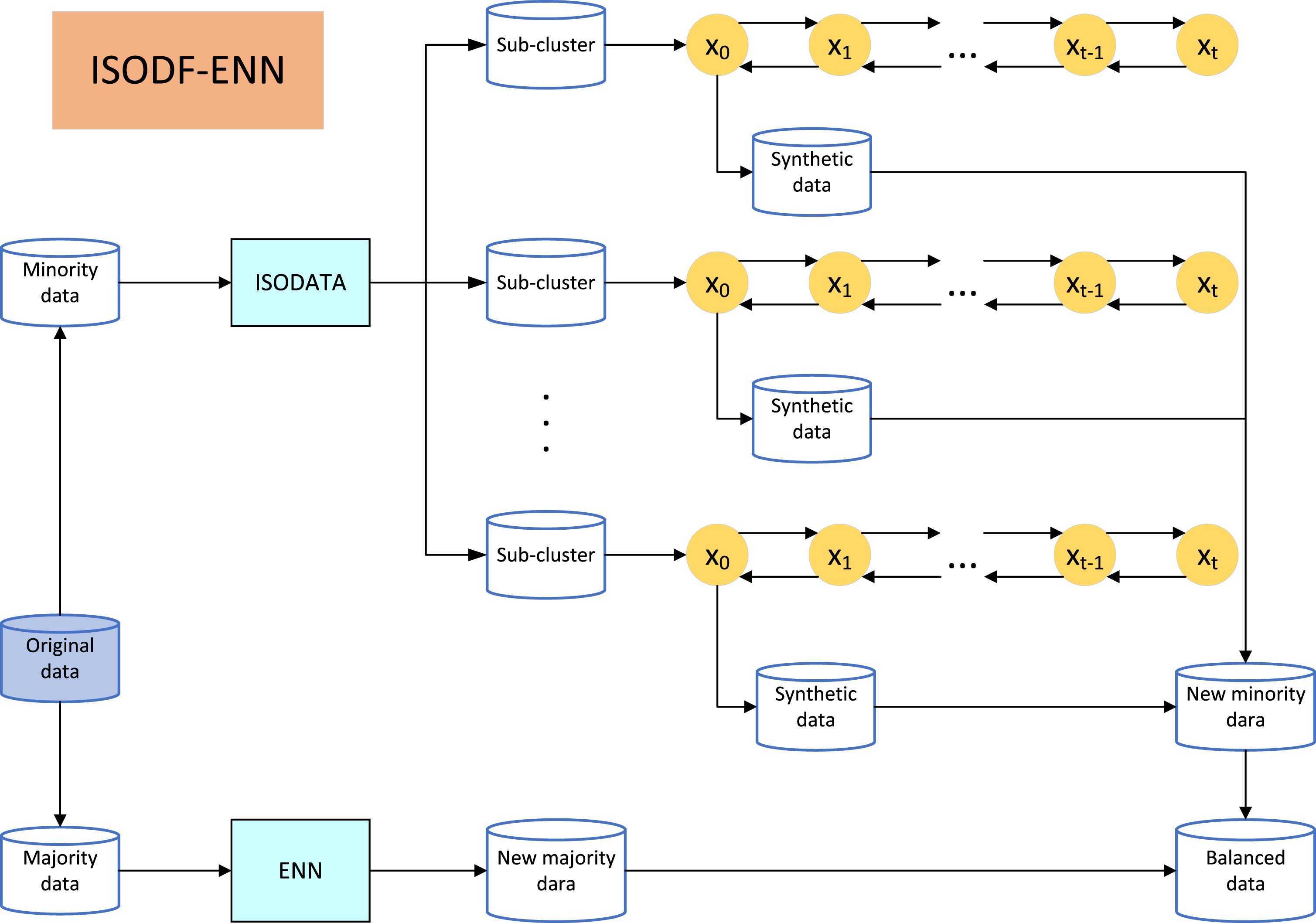
Basic process framework of ISODF-ENN.

3.1 K value determination

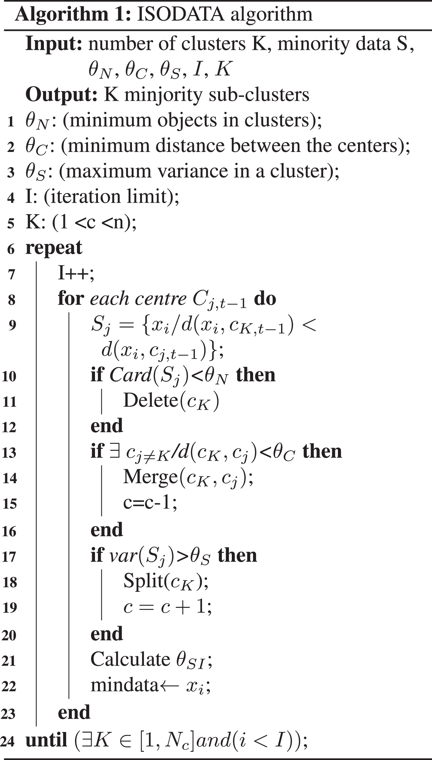
ISODATA is a dynamic clustering algorithm, the k is set to different value according to different datasets [23]. Therefore, we need a suitable method to determine the value of k. Silhouette coefficient is a commonly used method to select the appropriate number of clusters, which is suitable for distance-based clustering algorithms. This method calculates the average distance a(i) from the sample point to other samples in the same cluster and the average distance b(i) from the sample point to other cluster samples. The definition formula of silhouette coefficient is given in Equation 3. The larger the silhouette coefficient, the better the clustering effect. The optimal k value determined by silhouette coefficient make the clustering of ISODATA algorithm more accurate for data clustering and improve the performance and effectiveness of classifiers. $S\left(i\right)=\frac{b\left(i\right)-a\left(i\right)}{\mathit{max}\left\{a\right(i),b(i\left)\right\}}$(3)

3.2 ISODATA clustering stage

ISODATA algorithm is improved on the basis of k-means algorithm. In order to obtain a better clustering effect, this algorithm “merges” or “splits” sub-clusters according to the parameters to form new clusters. The iterative process is shown in Fig. 3.

Fig. 3

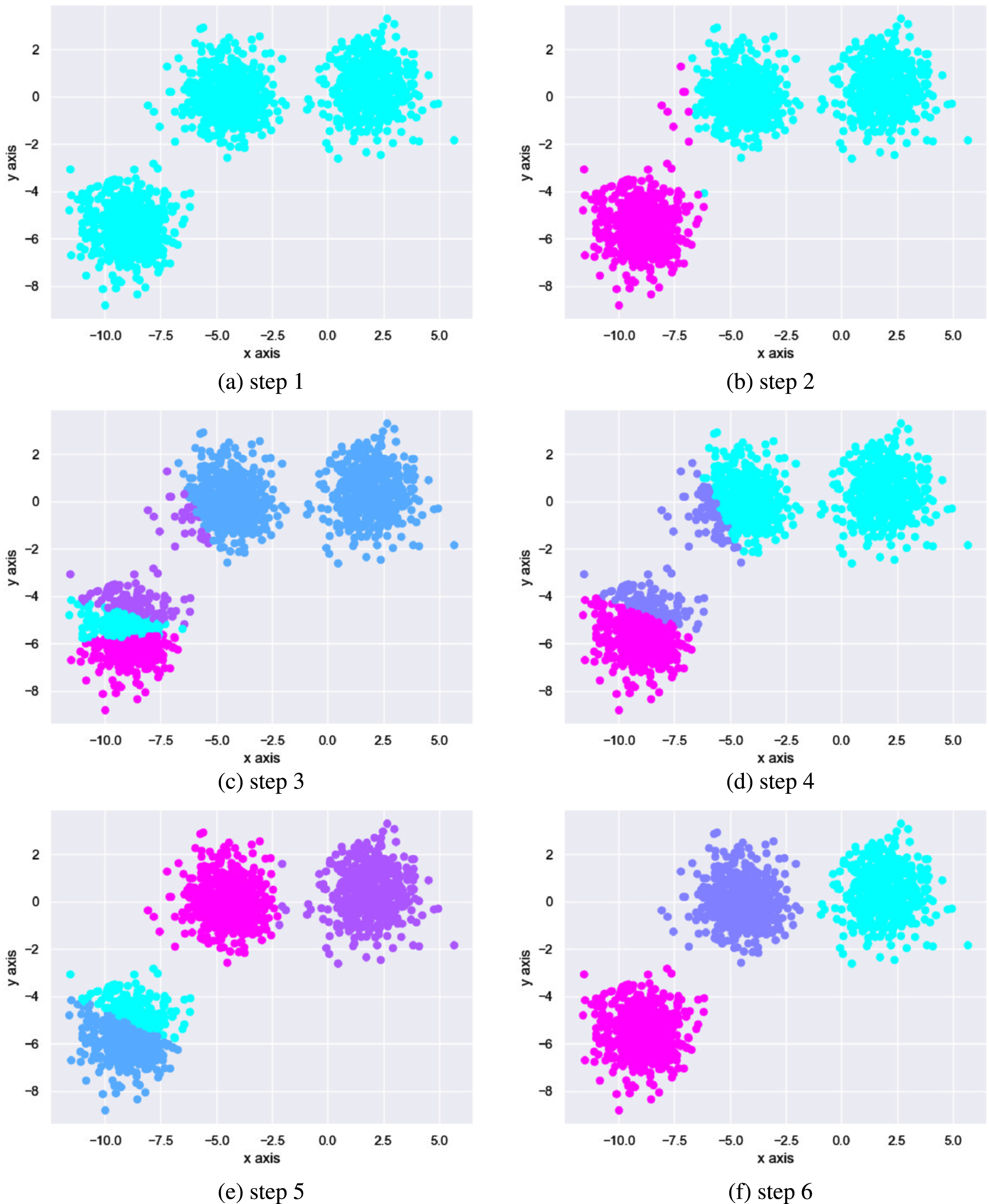
The iterative process of ISODATA algorithm.

The parameters that need to be determined and adjusted in the calculation are mainly include:

K: The expected number of cluster centers.

θ _N : The minimum number of samples that a class should have, otherwise, this class should be cancelled.

θ _S : A class sample standard deviation threshold, indicators of class division.

θ _C : Distance threshold for clustering centers, the minimum distance between two centers.

L: Maximum logarithm of cluster centers that can be merged in an iterative operation.

I: Maximum number of iterations allowed.

In the initial stage of ISODF-ENN algorithm, it is necessary to preprocess the training set. That is, minority classes in training set are clustered to be divided into different sub-clusters. In this algorithm, the number of sub-clusters is determined according to silhouette coefficient for each dataset, and then oversampled according to the sampling ratio. The purpose is to eliminate the imbalance between different classes of the dataset and the imbalance between different sub-clusters of the same class to ensure the quality of synthetic samples and prevent overfitting.

For ISODATA clustering algorithm, the basic process is as follows:

Input minority class data {x _i , i = 1, 2, . . . , N}, preselect N _c initial cluster centers {Z₁, Z₂, . . . , Z _{N c} }.

Assign N samples to the nearest sub-cluster S _j , if, $D_j=\mathit{min}\{\Vert x-Z_j\Vert ,i=1,2,\cdots N_c\},$(4) That is, the distance of ||x - Z _j || is the smallest, then x ∈ S _j .

If the number of samples N _j in S _j is less than θ _N , the sub-cluster is removed, and the number of sub-classes N _c is reduced by 1. The samples from the removed sub-class are reassigned to the remaining sub-class with the smallest distance.

Update each cluster center: $Z_j=\frac{1}{N_j}\sum _{x\in S_j}x,j=1,2,\cdots N_c$(5)

Calculate the average distance between the samples in each sub-cluster s _j and each cluster center: $\overline{D_j}=\frac{1}{N_j}\sum _{x\in S_j}\Vert x-Z_j\Vert ,j=1,2,...,N_c$(6)

Calculate the overall average distance of all sub-classes to other classes: $\overline{D}=\frac{1}{N}\sum _{j=1}^N{N}_j\overline{D_j}$(7)

Judgment of division, merge or cessation.

If the number of iterative operations has reached I times, that is, the last iteration, then set θ _C =0, and the algorithm ends.

If $N_c\le \frac{K}{2}$ , it means that the number of sub-classes is too small, and the class should be split.

If the number of iterations is even, or N _c  ≥ 2K, the algorithm proceeds to the tenth step without any splitting. However, if neither of these conditions are met, it goes to the eighth step to perform the splitting.

Splitting step:

Calculate the standard deviation of the samples in each class. For each sub-class S _j , the standard deviation is calculated by the following formula: ${\sigma }_j=[{\sigma }_{1j},{\sigma }_{2j},\cdots {\sigma }_{\mathit{nj}}{]}^{\top },j=1,2,\cdots N_c$(8)

The individual components of the vector are: ${\sigma }_{\mathit{ij}}=\sqrt{\frac{1}{N_j}\sum _{K=1}^{N_j}(x_{\mathit{iK}}-Z_{\mathit{ij}}{)}^2}$(9)

In Equation 9, i = 1, 2, . . . , n is the dimension of the sample feature vector, j = 1, 2, . . . , N _c is the number of sub-clusters, N _j is the number of samples in sub-cluster S _j .

Find the maximum component σ _jmax . For σ _jmax , if σ _jmax >θ _S , one of the following two conditions is satisfied:

$\overline{D_j}>\overline{D}$ andN _j >2 (θ _N  + 1)

$N_c\le \frac{K}{2}$

Split the sub-cluster S _j into two clusters, with the new cluster centers being represented by σ _jmax plus Kσ _jmax and σ _jmax minus Kσ _jmax . After the split, N _c  = N _c  + 1. If this step completes the split operation, then the algorithm go to the second step, otherwise, it continues.

Merging steps:

For all cluster centers, calculate the distance between any two cluster centers: $D_{\mathit{ij}}=\Vert Z_i-Z_j\Vert ,i=1,2,\cdots N_c-1,j=i+1,\cdots N_c$(10) Compare the values of D _ij and θ _C . If D _ij <θ _C , then arrange the value of D _ij in increasing order, and the arranged set is:{D _{i 1 j 1} , D _{i 2 j 2} , ⋯ D _{i L j L} }

In the set, D _{i 1 j 1} <D _{i 2 j 2} < ⋯ <D _{i L j L} . Merge from the smallest D _ij to get a new center: $Z_k^{*}=\frac{1}{N_{\mathit{ik}}+N_{\mathit{jk}}}[N_{\mathit{ik}}{Z}_{\mathit{ik}}+N_{\mathit{jk}}{Z}_{\mathit{jk}}],k=1,2,\cdots L$(11)

If it is the last iterative operation, this algorithm ends, otherwise, if the operator needs to change the input parameters, this algorithm return to the first step; if the input parameters remain unchanged, the algorithm proceed to the second step. In this step, the number of iterative operations should be incremented by 1 each time.

3.3 Denoising diffusion stage

Denoising diffusion model also known as diffusion model. The diffusion model is a generative model based on Markov chains. The diffusion model disrupts the original data by continuously adding Gaussian noise and then learns to reverse this noise to recover the data. Therefore, the model consists of three parts: the forward noise-addition process, the reverse denoising process, and the training process.

3.3.1 Forward noise-addition stage

The forward noise-addition process gradually introduces noise to the original data until it becomes completely random noise. Given data distribution x₀ ∼ q (x). Then the forward process refers to adding Gaussian noise to the data x_t-1 at time t-1 to obtain x _t , which is defined as q (x _t  - x_t-1). As t increases, x _t approaches pure noise. Given the hyperparameters of the Gaussian distribution, with a mean of $\sqrt{1-{\beta }_t}{x}_{t-1}$ and a variance of β _t , where β _t is also known as the linear timetable, its value increases with t. Generally, β _t is linearly interpolated between 0.0001 and 0.02. So, $q\left(x_t\right|x_{t-1})=N(x_t|\sqrt{1-{\beta }_t}{x}_{t-1},{\beta }_t\text{I})$(12)

I represents the identity matrix. The entire forward process of the diffusion model can be expressed as a Markov chain from t=1 to t=T. It can be expressed by Equation 13. $q\left(x_{0:T}\right)=q\left(x_0\right)\prod _{t=1}^{T}q\left(x_t|x_{t-1}\right)$(13)

An important feature of the diffusion model is that x _t at any time can be expressed by x₀ and β. Define α _t and $\overline{a}$ $\begin{array}{cc}\hfill {\alpha }_t=1-{\beta }_t& \hfill \\ \hfill \overline{a}=\prod _{s=1}^t{\alpha }_t& \hfill \end{array}$(14)

Through reparameterization, we can get any sample x _t obeying the distribution q (x _t |x₀).

$\begin{array}{cc}\hfill x_t& \sim q\left(x_t\right|x_0)\hfill \\ \hfill & ={\sqrt{\overline{\alpha }}}_t{x}_0+\sqrt{1-{\overline{\alpha }}_t}\varepsilon \hfill \\ \hfill & =N\left(x_t;{\sqrt{\overline{\alpha }}}_t{x}_0,\left(1-{\overline{\alpha }}_t\right)\text{I}\right)\hfill \end{array}$(15)

The noise adding process is shown in Fig. 4. It can be seen that as t increases, the original data gradually becomes random noise.

Fig. 4

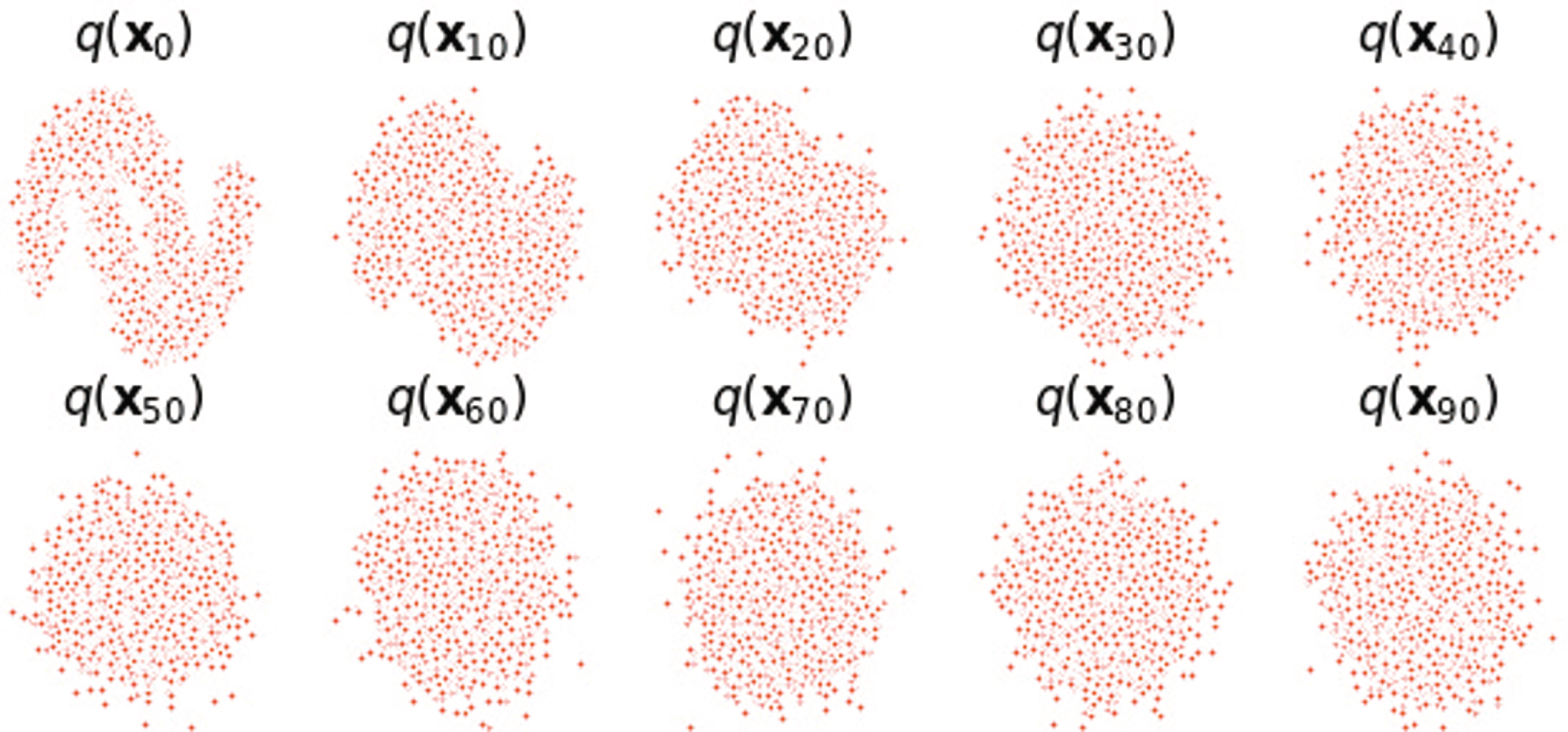
Data distribution after adding noise 90 times to the original data.

3.3.2 Reverse denoising stage

After adding noise, we need to restore the original data x₀ from the complete standard Gaussian distribution x _T  ∼ N (0, I), and we need to gradually obtain the reversed distribution q (x_t-1|x _t ). However, we cannot simply infer this process. Therefore, we need to use a deep learning model to learn the probability distribution p _θ from x _t to x_t-1. This process is shown in Fig. 5.

Fig. 5

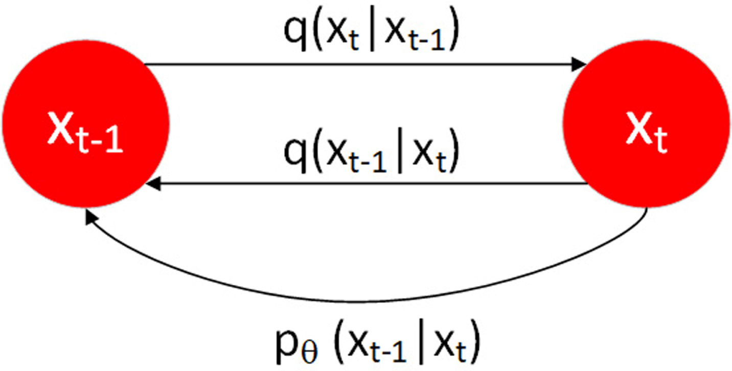
Schematic diagram of noise addition and denoising in the diffusion model, q (x_t-1|x _t ) is unknown, and use deep learning to predict the probability distribution p _θ .

Assuming that the noise removed by the reverse process also conforms to the Gaussian distribution, and the Gaussian distribution is determined by the mean μ _θ and the variance ∑ _θ , then p (x_t-1|x _t ) can be expressed as: $p_{\theta }\left(x_{t-1}|x_t\right)=N\left(x_{t-1};{\mu }_{\theta }\left(x_t,t\right),\sum _{\theta }\left(x_t,t\right)\right)$(16)

Combining all time steps, we can get: $p_{\theta }\left(x_{0:T}\right)=p\left(x_T\right)\prod _{t=1}^T{p}_{\theta }\left(x_{t-1}|x_t\right)$(17)

Although we cannot get the reversed distribution q (x_t-1|x _t ), if we know x₀, we can infer:

$\begin{array}{cc}\hfill q\left(x_{t-1}\right|x_t,x_0)& =N\left(x_{t-1};\tilde{\mu }\left(x_t,x_0\right),{\tilde{\beta }}_t\text{I}\right)\hfill \\ \hfill & =\frac{q\left(x_t|x_{t-1},x_0\right)q\left(x_{t-1}|x_0\right)}{q\left(x_t|x_0\right)}\hfill \\ \hfill & \propto N\left(x_{t-1};{\mu }_q\left(x_t,x_0\right),\sum _q\left(t\right)\right)\hfill \end{array}$(18)

The mean μ _q  (x _t |x₀), variance ∑ _q  (t) and x₀ are: ${\mu }_q\left(x_t\right|x_0)=\frac{{\sqrt{\alpha }}_t\left(1-{\overline{\alpha }}_{t-1}\right)x_t+\sqrt{{\overline{\alpha }}_{t-1}}\left(1-{\alpha }_t\right)x_0}{1-{\overline{\alpha }}_t}$(19) $\sum _q\left(t\right)=\frac{\left(1-{\alpha }_t\right)\left(1-{\overline{\alpha }}_{t-1}\right)}{1-{\overline{\alpha }}_t}\text{I}$(20) $x_0=\frac{x_t-\sqrt{1-\overline{{\alpha }_t}}{\varepsilon }_0}{\sqrt{\overline{{\alpha }_t}}}$(21)

We bring x₀ into the mean. $q\left(x_t,x_0\right)=\frac{1}{\sqrt{{\alpha }_t}}{x}_t-\frac{1-{\alpha }_t}{\sqrt{1-\overline{{\alpha }_t}}\sqrt{{\alpha }_t}}{\varepsilon }_0$(22)

It can be seen from Equation 22 and the definition of variance, the mean is dependent on the data, while the variance depends on a linear timetable.

The denoising process is shown in Fig. 6.

Fig. 6

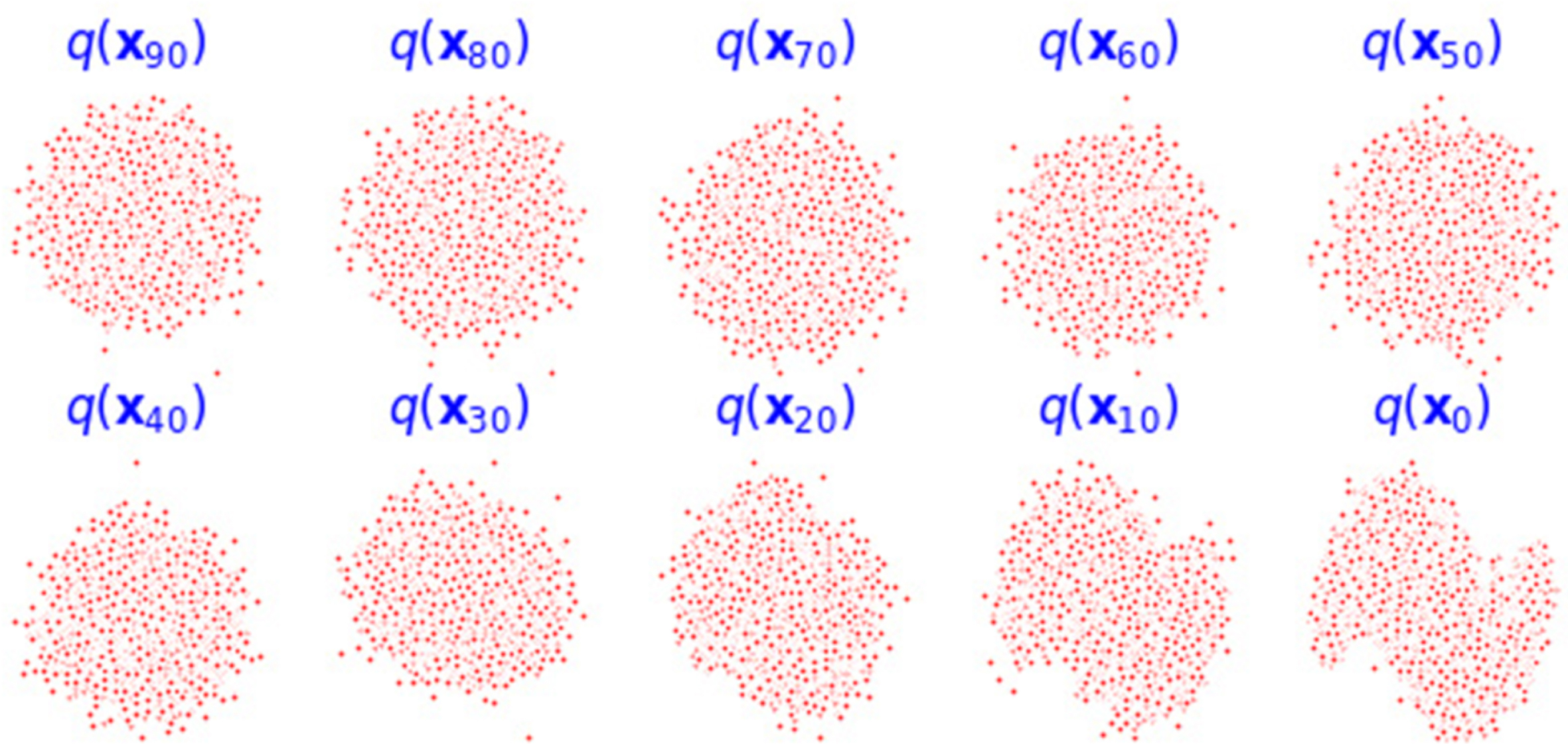
The data distribution of the noise-added data after reverse denoising.

3.3.3 Training stage

We model the denoising process using neural networks, aiming to minimize the disparity between actual noise and estimated noise by maximizing the evidence lower bound of the variational autoencoder. This optimization enhances both mean and variance. The loss function is illustrated in Equation 23. ${\mathcal{L}}_{\mathit{simple}}=E_{t,x_0,\varepsilon }{\parallel {\varepsilon }_t-\hat{\varepsilon }\left({\sqrt{\overline{\alpha }}}_t{x}_0+\sqrt{1-\overline{{\alpha }_t}}\varepsilon ,t\right)\parallel }^2$(23)

This algorithm uses Backpropagati (BP) neural network for noise prediction. BP neural network is a commonly used feedforward neural network, consisting of an input layer, a hidden layer and an output layer. Input data is passed through the network from the input layer to the output layer. Each neuron receives input from the previous layer, adds a bias variable through a weighted sum, and then performs nonlinear processing through an activation function to obtain an output. The error is propagated backwards from the output layer to the hidden and input layers by computing the difference between the output and the target. This is achieved by computing the gradient of each neuron and distributing the error to each connection weight.

To prevent overfitting, we use random deactivation. During the learning process of the neural network, the weights of some hidden layer nodes are randomly reset to zero. Since the nodes affected by zeroing are different in each iteration, each node of the neural network will contribute content. In this experiment, the coefficient of random deactivation is 0.5, that is, half of the neural nodes are deactivated randomly.

3.4 Data cleaning stage

In imbalanced datasets, the number of samples in minority classes is very small, which makes them very susceptible to data overlap. As a result, the classifier cannot accurately distinguish between different classes. In some imbalanced datasets, the boundaries between minority and majority classes may be blurred. When data overlap occurs, conventional classification algorithms may be influenced by majority class, which will cause the minority class data to be ignored. Therefore, after minority class synthetic data, we use ENN algorithm to clean the data.

3.5 Time complexity analysis

The ISODATA clustering algorithm requires calculating distances between data points within each sub-cluster and distances between the centroids of different sub-clusters in each iteration. Therefore, the time complexity of the ISODATA algorithm is O (n²). The diffusion algorithm is applied to each sub-cluster to generate new minority-class data points. The denoising diffusion algorithm consists of a noise-adding process and a denoising process. The time complexity of the noise-adding process depends only on the step size and requires linear time. The denoising process involves training a BP neural network to reverse the noise-adding process, resulting in a time complexity of O (n²). The ENN algorithm needs to search for the nearest neighbor of each data, so the time complexity of this process is O (n²) Consequently, the time complexity of the ISODF-ENN algorithm is O (n²).

4 Experimental analysis

4.1 Experimental data

To examine classification performance of ISODF-ENN algorithm, this paper select 8 groups of imbalanced datasets on KEEL (https://www.keel.es) [24] for experiments. The number of these datasets ranges from small to large, and from slightly imbalanced to highly imbalanced. Table 1 gives the basic information of these datasets. The first list shows the name of datasets, and the second list shows the number of samples of datasets. The third list shows the number of features of datasets. The fourth list is the imbalance degree of the dataset, and the fifth list is the number of sub-clusters after clustering of the dataset. Formula 24 is the calculation method of the imbalance degree of datasets. Figure 7 shows the best k value for the dataset by silhouette coefficient.

$I.R=\mathit{Nax}/\mathit{Nin}$(24)

Fig. 7

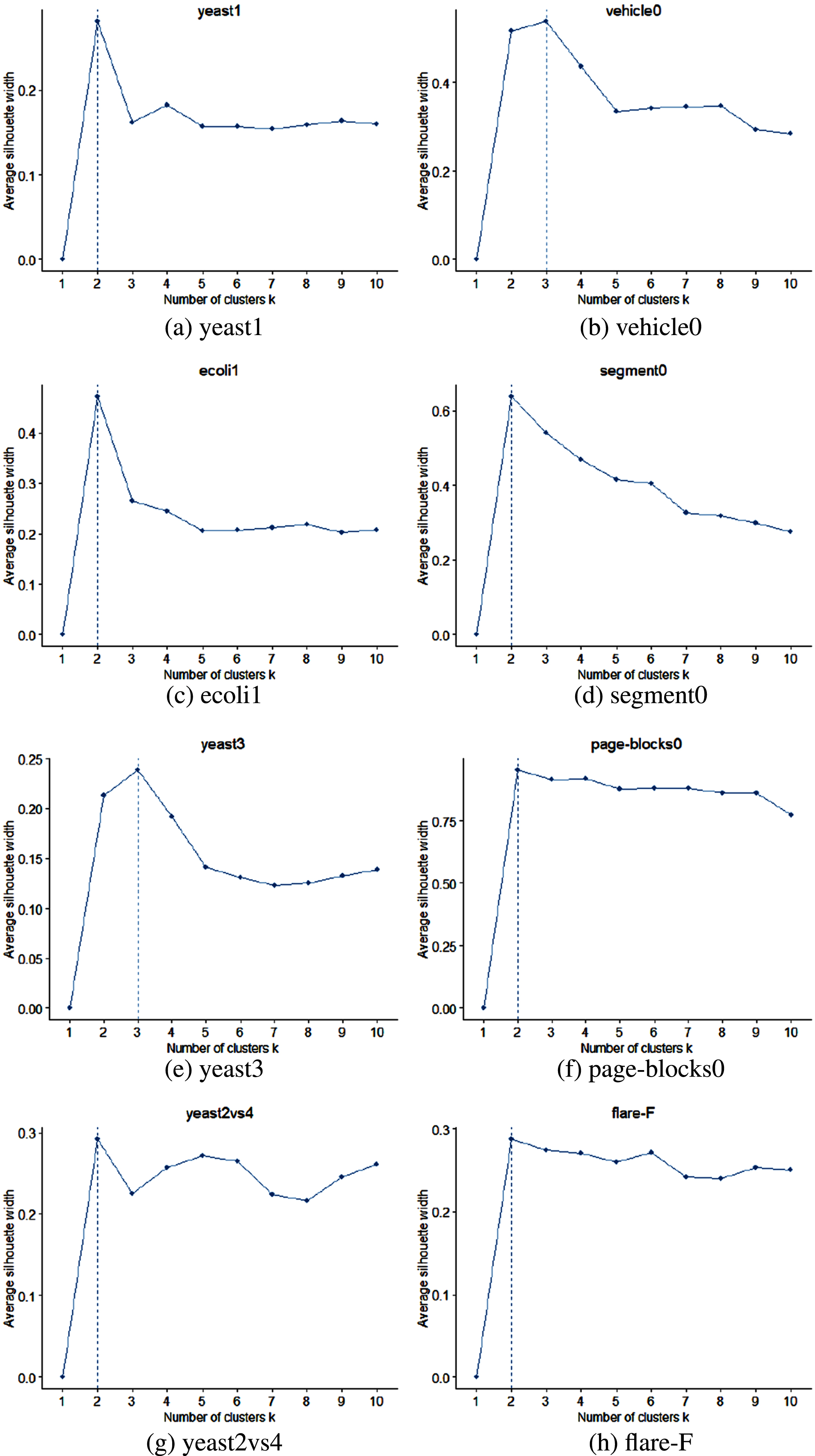
The optimal k values to datasets through the silhouette coefficient.

Table 1

Description of experimental data set

Data set	No.of instances	No.of attributers	I.R	K
yeast1	1484	8	2.46	2
vehicle0	846	18	3.25	3
ecoli1	336	7	3.36	2
segment0	2308	19	6.02	2
yeast3	1484	8	8.1	3
page-blocks0	5472	10	8.79	2
yeast2vs4	514	8	9.08	2
flare-F	1066	11	23.79	2

Define R _aug for assessing the overlap ratio of imbalanced data, where a higher value indicates a greater degree of data overlap [25]. The calculation equation is: $R_{\mathit{aug}}=\frac{R\left(C_0\right)+\mathit{IR}*R\left(C_1\right)}{\mathit{IR}+1}$(25)R (C _i ) represents the overlap ratio of class i, which is defined as Equation 26. $R\left(C_i\right)=\frac{1}{\left|C_i\right|}\sum _{m=1}^{\left|C_i\right|}\mathit{sgn}\left(\mathit{knn}\left(X_{\mathit{im}},\overline{C_i}\right)-\theta \right),\left(i=0,1\right)$(26)

C₀ and C₁ represent majority class samples and minority class samples, and X _im is the m-th sample of C _i . $\overline{C_i}$ is the complement set of C _i , $\mathit{knn}(X_{\mathit{im}},\overline{C_i})$ represents the k nearest neighbor set of X _im , and the set belongs to $\overline{C_i}$ . θ is the threshold regarding the number of neighbors of different classes that consider a sample to belong to the overlapping region. The calculation method of sgn (x) is as Equation 27. The nearest neighbor k and threshold θ are the key to calculating R _aug . Usually, the value range of θ is [0, k/2]. In further simulations and studies, the values of k and θ were 7 and 3. $\mathit{sgn}\left(x\right)\{\begin{array}{c}1\mathit{if}x>0\\ 0\mathit{otherwise}\end{array}$(27)

The overlapping area of the dataset is shown in Table 2, where R _neg is the overlapping area of the majority class data, R _pos is the overlapping area of the minority class data, and the calculation formula is shown in Equation 26.

Table 2

Overlap ratio percentage of datasets

Data set	R neg	R pos	R aug
yeast1	11.47	56.18	43.26
vehicle0	3.86	9.55	8.21
ecoli1	3.86	24.68	19.90
segment0	0.96	3.04	2.74
yeast3	1.67	30.67	27.49
page-blocks0	1.16	28.98	26.14
yeast2vs4	0.65	37.25	33.62
flare-F	0.00	100	95.96

In the experiment, in order to ensure the accuracy of experimental results as much as possible, we use 5-fold cross-experimental verification, and the experiment is repeated 10 times, and the final experimental result is the average value of these 10 experiments.

4.2 Performance measures

In the two-class problem, classification results of classifiers on the sample have four cases, which are displayed by the confusion matrix, as shown in Table 3. TP and TN represent the number of correctly classified samples belonging to the minority class and the majority class respectively. FP represents the number of samples of the majority class predicted as the minority class, and FN is the number of minority class data predicted as the majority class.

Table 3

Confusion matrix

	Predicted Positive	Predicted Negative
Actual Positive	TP	FN
Actual Negative	FP	TN

According to Table 3, the following evaluation indexes can be obtained:

$\mathit{Precision}=\frac{\mathit{TP}}{\mathit{TP}+\mathit{FP}}$

$\mathit{FalsePositiveRate}\left(\mathit{FPR}\right)=\frac{\mathit{FP}}{\mathit{FP}+\mathit{TN}}$

$\mathit{Recall}\left(\mathit{TPR}\right)=\frac{\mathit{TP}}{\mathit{TP}+\mathit{FN}}$

$F-\mathit{value}=\frac{2*\mathit{Precis}*\mathit{Recall}}{\mathit{Precision}+\mathit{Recall}}$

TPR is the true positive rate, which represents the proportion of correctly classified minority classes in minority data. TNR is the true negative rate, which represents the proportion of correctly classified majority classes in majority data.

F-value is based on the harmonic average of precision and recall. It is a comprehensive evaluation index of precision and recall, which can more accurately display the classification accuracy of positive sample. The AUC value is a common indicator used to evaluate the pros and cons of the binary classification model. The higher the AUC value, the better the effect of the model. Its value is the area under the ROC curve. The abscissa of the ROC curve is FPR and the ordinate is TPR. By adjusting the positive class probability threshold of the classifier, multiple sets of FPR and TPR are obtained, and the ROC curve is drawn to obtain the AUC value [26].

4.3 Parameter sensitivity experiment

ISODATA algorithm relies on continuously updating the center position of the cluster to obtain better clustering effect. This algorithm considers the intra-class imbalance of minority data, and clusters minority data to oversamples in the sub-cluster. Therefore, the quality of clustering directly affects the results of subsequent oversampling [27]. If the clustering effect is poor, the distribution of the synthesized minority data is quite different from the distribution of the original minority data. This will generate a lot of noise, and cover up the data characteristics of the original minority data, and affect classification performance of classifiers on the minority data. It is necessary to determine the appropriate parameters of ISODATA to obtain the best clustering effect.

In this section, we discuss the potential impact of the sample standard deviation threshold θ _S , the cluster center distance threshold θ _C and the number of iterations I on the performance of ISODF-ENN, and select appropriate parameters. Since θ _S and θ _C influence each other, we are talking about the multiple relationship between θ _S and θ _C . Because the distance between two cluster centers is greater than the standard deviation between samples, Mul is defined as the multiple of θ _C greater than θ _S . Mul takes values at 5, 20, 50, 100, and I takes values at 5, 10, 20, 30. The corresponding results are shown in Tables 4 and 5.

Table 4

The impact of Mul on AUC for ISODF-ENN by DT

Data set	Mul	AUC	Data set	Mul	AUC
yeast1	5	0.6796	yeast3	5	0.9014
	20	0.6894		20	0.9112
	50	0.6876		50	0.9128
	100	0.6949		100	0.9205
vehicle0	5	0.9102	page-blocks0	5	0.9298
	20	0.9476		20	0.9345
	50	0.9198		50	0.9213
	100	0.9214		100	0.9376
ecoli1	5	0.8624	yeast2vs4	5	0.9011
	20	0.8614		20	0.8922
	50	0.8789		50	0.9102
	100	0.8752		100	0.9161
segment0	5	0.9745	flare-F	5	0.7014
	20	0.9842		20	0.7142
	50	0.9802		50	0.7269
	100	0.9741		100	0.7245

Table 5

The impact of I on AUC for ISODF-ENN by DT

Data set	5	10	20	30
yeast1	0.6918	0.6911	0.6949	0.6921
vehicle0	0.9321	0.9488	0.9476	0.9411
ecoli1	0.8615	0.8702	0.8798	0.8645
segment0	0.9721	0.9810	0.9842	0.9702
yeast3	0.9175	0.9144	0.9205	0.9133
page-blocks0	0.9189	0.9256	0.9376	0.9378
yeast2vs4	0.9045	0.9112	0.9161	0.9055
flare-F	0.7105	0.7212	0.7269	0.7111

For clarity, the AUC results of the DT classifier are presented here. And the best results for the parameters on each dataset are highlighted in bold. As can be seen from Tables 5, there are no universal optimal parameters for all data sets. However, Mul is between 50-100 and I is 20, which performs better on most data sets. The specific settings depend on the researchers’ needs in actual application scenarios.

4.4 Analysis of experimental results

In order to verify the feasibility of the ISODF-ENN algorithm, we used the original data as a baseline and selected seven different sampling methods as the comparison group, including SMOTE [12], KNSMOTE [15], KmUnder [16], TL [17], SMOTE+ ENN [28], GAN [19], TWGAN-GP [20]. Verify the above algorithms on datasest shown in Table 1, and combines the DT classification algorithm to obtain the F-value and AUC. Because division of the dataset and synthesis of new samples in the experiment are accidental, this experimental results are performed ten times and averaged. The results are shown in Table 6, and best values are shown in bold.

By comparing the above algorithms, it can be observed that ISODF-ENN algorithm has a good effect on the classification of imbalanced datasets. In Table 6, ISODF-ENN achieved the best F-value on 5 datasets and the best AUC on 7 datasets. In datasets that the best values were not achieved, the IR of yeast1 was 2.46, R _aug was 43.26, the IR of vehicle0 was 3.25, R _aug was 8.21, the IR of flare-F was 23.79, R _aug was 95.96, and the IR of segment0 was 6.02, R _aug was 2.74. It can be observed that, except for the flare-F dataset, the IR or R _aug of ISODF-ENN in datasets where it did not achieve the best performance is relatively low. Particularly, when the IR is lower, the algorithm’s performance improvement is less noticeable. On the flare-F dataset, the F-value of ISODF-ENN is close to the best value, indicating that this algorithm significantly improves performance on datasets with high imbalance and overlap.

4.5 Significance test

To better assess whether there are significant differences between ISODF-ENN and other methods, we employed the Friedman test. The Friedman test is based on ranking performance rather than actual performance evaluation, making it less susceptible to the influence of outliers. In this experiment, we first calculated the performance rankings of the nine methods in each dataset and then presented the final rankings in the form of averages. The average rankings of F-value and AUC are shown in Figs. 8 9.

Fig. 8

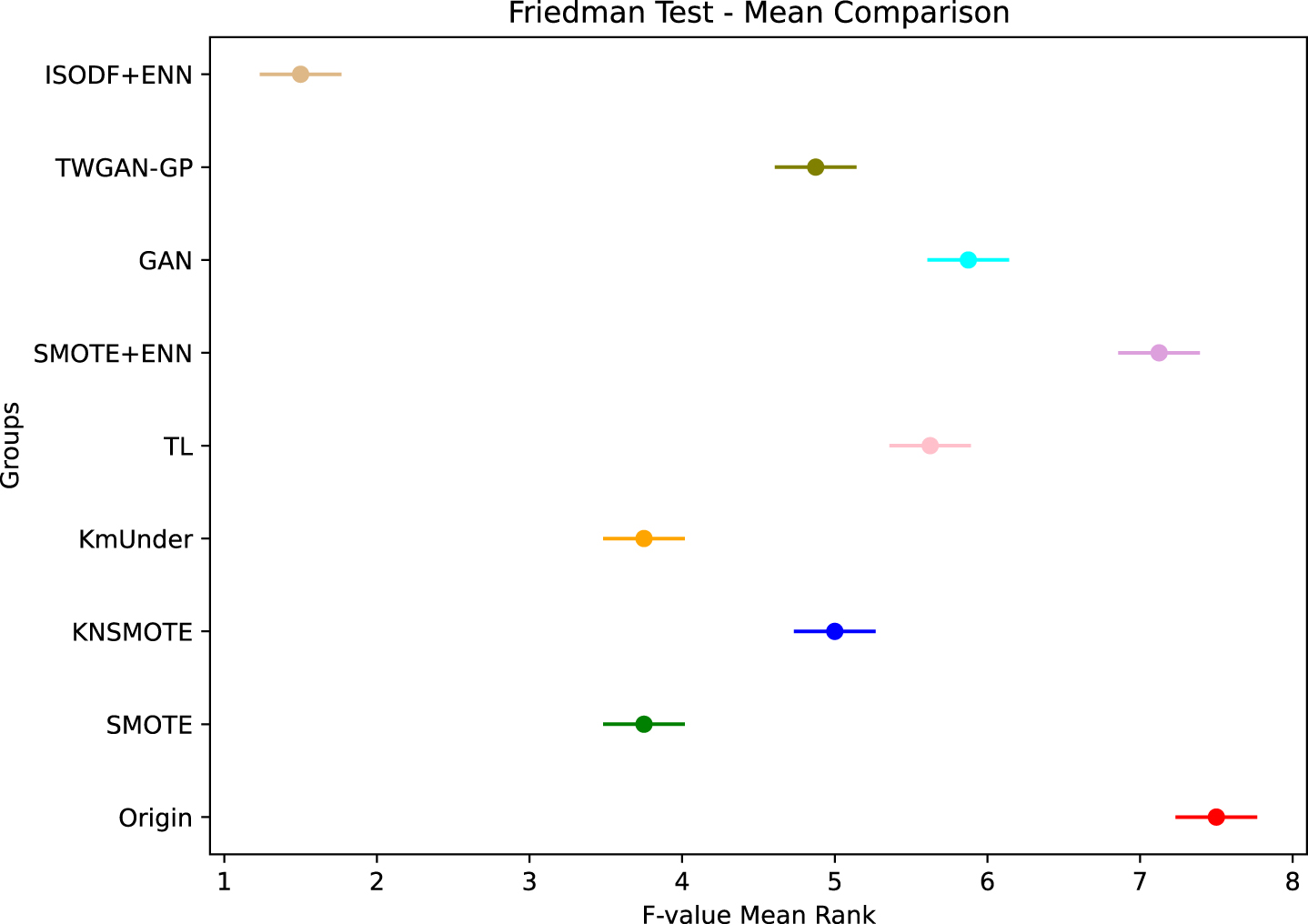
Friedman test of F-value of different algorithms.

Fig. 9

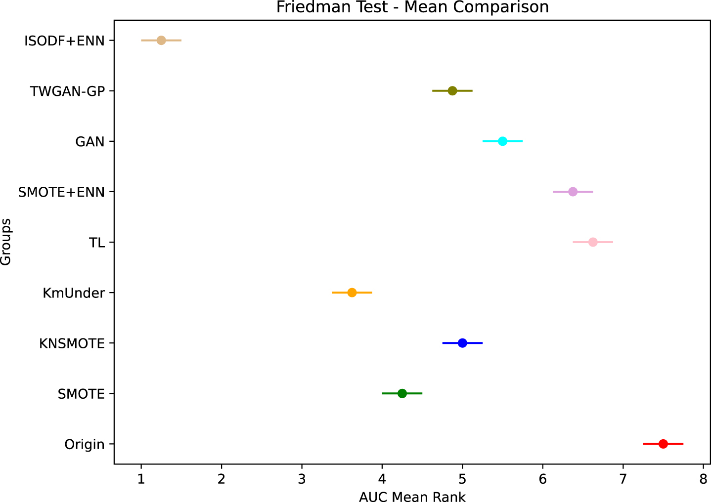
Friedman test of AUC of different algorithms.

It can be observed that our algorithm achieves a significant advantage in both the F-value and AUC evaluation metrics. This indicates that the excellence of ISODF-ENN is highly consistent across various performance measures.

Furthermore, in this section, quantitative analysis was conducted using the Friedman test. We analyzed the differences between the nine methods based on the significance value p. If the corresponding p-value is less than 0.05, it indicates the presence of a difference; if the corresponding p-value is greater than 0.05, it suggests no significant difference. The specific test results are shown in Table 7. From the p-values, it can be confirmed that the performance differences among the nine methods are not random, and there is a significant difference between different methods.

Table 6

Evaluation index results of different algorithms combined with DT classifier on the data set

	Data set	Origin	SMOTE	KNSMOTE	KmUnder	TL	SMOTE+ENN	GAN	TWGAN-GP	ISODF-ENN
F-value	yeast1	0.4919	0.5126	0.5491	0.5913	0.5125	0.5023	0.5152	0.5574	0.5852
	vehicle0	0.6781	0.8409	0.8557	0.8511	0.6541	0.6630	0.7666	0.8163	0.8451
	ecoli1	0.6137	0.7315	0.7168	0.7211	0.6896	0.6848	0.7028	0.7332	0.7558
	segment0	0.8777	0.9689	0.9478	0.9330	0.9675	0.7950	0.8559	0.8709	0.9705
	yeast3	0.6664	0.7016	0.7241	0.7014	0.6802	0.6810	0.6726	0.7285	0.7408
	page-blocks0	0.4883	0.5026	0.4579	0.6194	0.4459	0.4335	0.5196	0.4428	0.8144
	yeast2vs4	0.6316	0.6934	0.6002	0.6523	0.7107	0.6161	0.6413	0.6210	0.7238
	flare-F	0.1059	0.1944	0.1308	0.1402	0.2071	0.2876	0.1761	0.1813	0.2725
AUC	yeast1	0.6439	0.6559	0.6846	0.6923	0.6561	0.6466	0.6592	0.6874	0.6949
	vehicle0	0.7923	0.9199	0.9215	0.9101	0.7666	0.7955	0.8616	0.9260	0.9476
	ecoli1	0.7476	0.8305	0.8290	0.8336	0.8099	0.7997	0.8101	0.8341	0.8798
	segment0	0.9040	0.9821	0.9855	0.9861	0.9815	0.8451	0.9247	0.8990	0.9842
	yeast3	0.8314	0.8557	0.8771	0.8123	0.8201	0.8573	0.8403	0.8826	0.9205
	page-blocks0	0.7942	0.7833	0.7706	0.8253	0.7187	0.7607	0.8457	0.7582	0.9376
	yeast2vs4	0.7839	0.8684	0.7623	0.8889	0.8505	0.7952	0.7857	0.7821	0.9161
	flare-F	0.5369	0.6500	0.5713	0.6231	0.5833	0.6443	0.5747	0.5763	0.7269

Table 7

Friedman test quantitative analysis

Metric	p	Hypothesis(0.05)
F-value	3 × e-04	Rejected
AUC	2.7 × e-04	Rejected

4.6 Ablation study

To investigate the effectiveness of various modules, we conducted ablation experiments. Using the original data as the baseline, evaluation metrics for ENN, the diffusion model based on ISODATA (ISODF), and ISODF-ENN are shown in the Figs. 10 11.

It can be observed that the evaluation metrics of ENN and ISODF are superior to the original data on the most of datasets, and ISODF-ENN outperforms ENN and ISODF on all datasets. This indicates the effectiveness of various modules, which play a positive role in enhancing the classifier’s classification performance.

Fig. 10

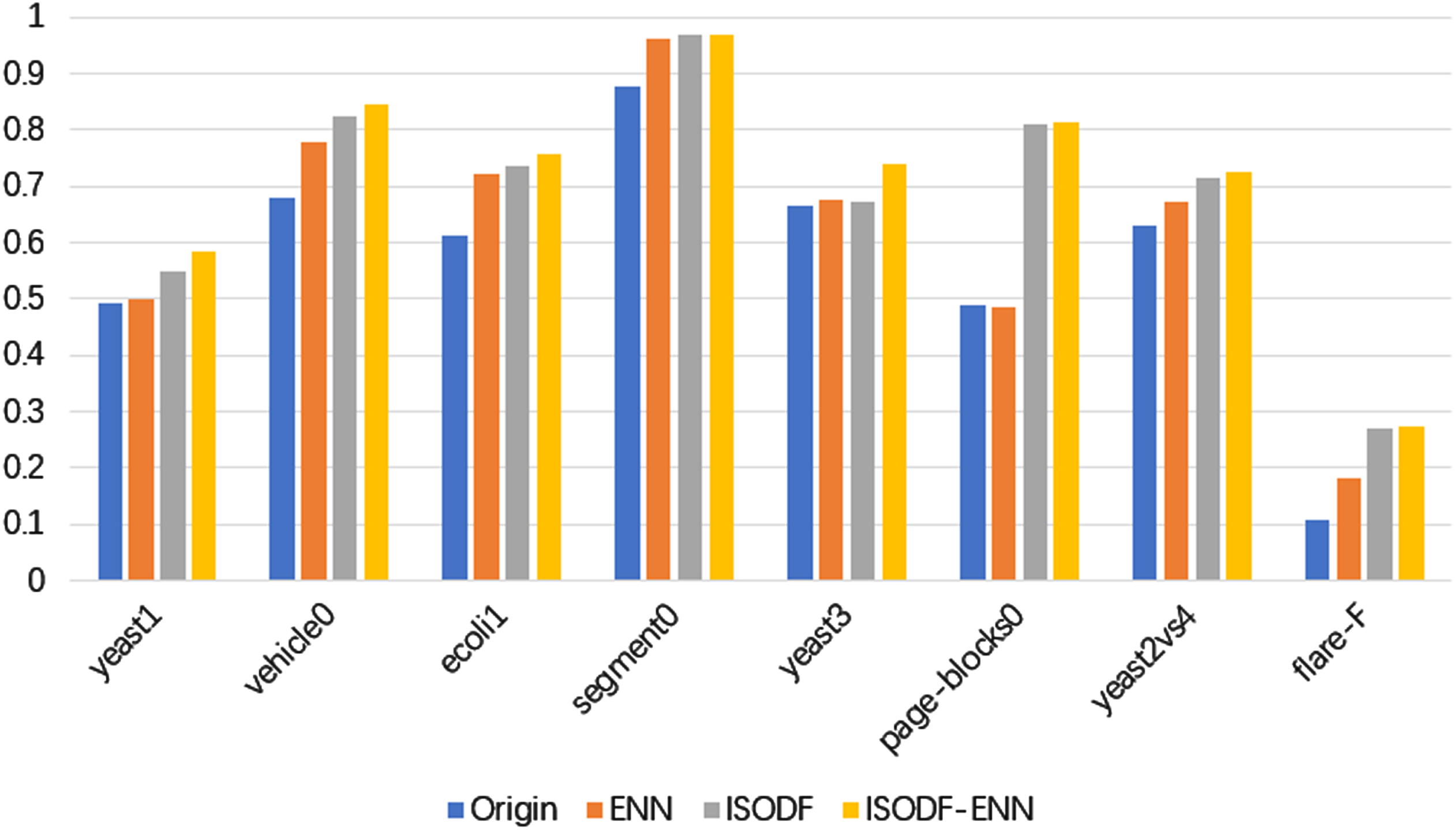
F-value of each algorithm after ablation experiment.

Fig. 11

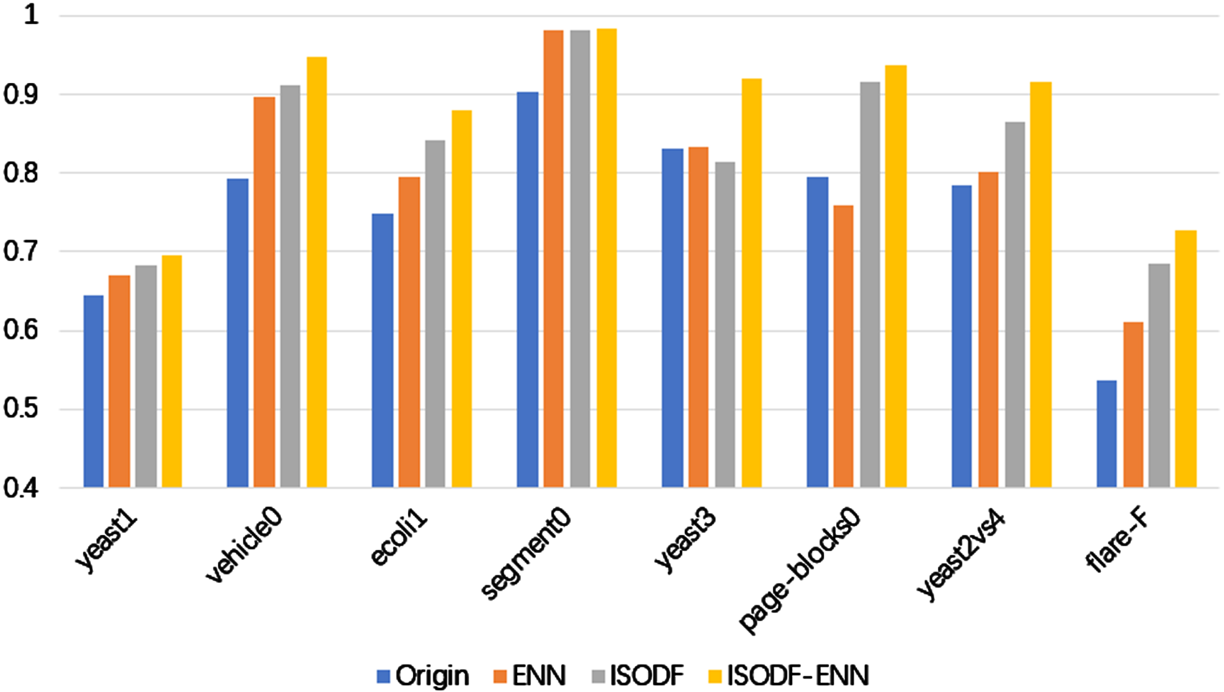
AUC of each algorithm after ablation experiment.

5 Conclusion

Aiming to solve the problem of performance degradation of traditional classifiers on imbalanced datasets and improve the accuracy of minority class data classification, this paper proposes a mixed sampling method based on ISODATA clustering. ISODF-ENN uses oversampling method to synthesize new minority class data and form a new balanced dataset. Meanwhile, clustering was performed on the minority class data, followed by applying a denoising diffusion algorithm to generate new minority class data for each sub-cluster, and the ENN algorithm was used to clean the boundary data. This effectively solves the problem of blurred class boundaries and improves the quality of the synthesized data. After verification, this algorithm has high accuracy in the classification of minority class samples, and this algorithm can be used in the classification of imbalanced data.

Acknowledgments

This work is supported by National Natural Science Foundation of China (No. 62103350) and Shandong Provincial Natural Science Foundation (ZR2020QF046).