Predicting the california bearing ratio via hybrid method of multi-layer perceptron

Abstract

The California Bearing Ratio (CBR) holds significant importance in the design of flexible pavements and airport runways, serving as a critical soil parameter. Moreover, it offers a means to gauge the soil response of subgrades through correlation, an aspect pivotal in soil engineering, particularly in shaping subgrade design for rural road networks. The CBR value of soil is influenced by numerous factors, encompassing variables like maximum dry density (MDD), optimum moisture content (OMC), liquid limit (LL), plastic limit (PL), plasticity index (PI), soil type, and soil permeability. The condition of the soil, whether soaked or unsoaked, also contributes to this value. It is worth noting that determining CBR is time-consuming and extensive. Acknowledging the gravity of this determination, the study introduces a pioneering approach employing machine learning. This innovative technique uses a foundational multi-layer perceptron model, harnessing the algorithm’s robust capabilities in addressing regression challenges. A hybridization approach enhances the multi-layer perceptron’s performance and achieves optimal results. This approach integrates the Bonobo Optimizer (BO), Smell Agent Optimization (SAO), Prairie Dog Optimization (PDO), and Gold Rush Optimizer (GRO). The hybrid models proposed in this study exhibit promising results in predicting CBR values. The MLAO3 hybrid model is particularly noteworthy, emerging as the most accurate predictor among the range of models, with an impressive R² value of 0.994 and an RMSE value of 2.80.

1 Introduction

In geotechnical engineering, a soil specimen’s capacity to resist a piston’s penetration is defined as the California Bearing Ratio (CBR). Specifically, the CBR represents the force necessary to drive the piston into the soil [1]. Initially conceived in California to assess soil suitability for highway construction, the CBR test was adapted by civil engineers to enhance its applicability in airport construction. Developing nations have widely adopted the CBR test for evaluating pavement soil resistance [2–5]. The CBR is the ratio of the bearing capacity of the available base material to that of a standard material (crushed rock). In structural engineering, a CBR value of 100 is allowable for crushed rock, whereas values for other materials are below 100 [6, 7].

The CBR test is conducted through two distinct methods: in the field or the laboratory. Laboratory testing is performed on compacted soils, while field testing is utilized for soils within trenches. Notably, variations in soil type, dry unit weight, and water content can lead to discrepancies between field and laboratory test results [8]. CBR testing can be carried out on unsoaked and soaked soil types, offering valuable insights into the resistance of various soil-related structures, such as road fillings, dams, airport pavements, and highway barriers. Despite its significance, the CBR determination process is time-intensive and labor-demanding, often yielding inaccurate values due to suboptimal laboratory conditions and soil samples [9, 10].

Prior research has focused on exploring various aspects of CBR, highlighting its sensitivity to soil types and properties. Much of the study has centered on the relationships between compaction characteristics, specific indices, and CBR values of soil samples [11–14]. Soils are compacted to predetermined maximum dry density (MDD) and optimum moisture content (OMC) levels using specific energy, which aids in assessing CBR. In the case of soaked CBR, samples are left to soak for four days, resulting in a total testing time of 5–6 days, potentially causing significant delays in large construction projects [15–17].

Given the substantial variability in soil characteristics, conducting the CBR test on subbase soil samples from a limited range of locations may not accurately represent all road conditions. To address this limitation, it is crucial to test a substantial number of specimens. Thus, estimating CBR values for pavement subgrade materials using easily identifiable parameters becomes paramount. Artificial intelligence (AI) methods have gained traction in addressing geotechnical engineering challenges empirically. Some studies have explored the estimation of CBR values using various artificial neural network (ANN) applications [18–20].

For instance, Baghbani et al. [21] employed support vector machines, artificial neural networks, and genetic programming to predict CBR based on a dataset with nine input variables. Their results demonstrated the efficacy of AI methods, with R² values ranging from 0.94 to 0.99 and MAE values ranging from 0.30 to 0.51. Khatti and Grover [22] compared LSTM, LSSVM, and ANN models to predict CBR. They achieved R² and RMSE values of 0.99 and 0.91, respectively. Nagaraju et al. [23] introduced an integrated extreme learning machine-cooperative search optimizer (ELM-CSO) method for CBR prediction, showing that ELM-CSO outperformed CSO with R² and RMSE values of 0.97 and 0.84. Kim et al. [24] predicted CBR for fine and coarse aggregates, achieving satisfactory accuracy with R² values of 0.938 and 0.829, respectively. Othman and Abdelwahab [25] focused on using ANN models for efficiently estimating subgrade soil CBR in Egypt based on Atterberg limits, grain size distribution, and compaction components.

Given the diverse variables and rich datasets available in previous research, developing robust predictive tools to model CBR mechanical properties and capture complex relationships between soil constituents is crucial. This paper presents a machine-learning-based model for estimating CBR using an experimental dataset from reputable sources cited above. To achieve this, a multi-layer perceptron (MLP) model is employed, incorporating Bonobo Optimizer (BO), Prairie Dog Optimization (PDO), Gold Rush Optimizer (GRO), and Smell Agent Optimization (SAO) for accurate CBR value predictions. Determining CBR values is a crucial aspect of civil engineering, but its traditional approach is labor-intensive and financially burdensome. Predicting CBR values offers a promising avenue to reduce costs and streamline project timelines. This study introduces a precise model as a viable alternative to conventional CBR determination techniques. The model effectively estimates CBR values using input variables encompassing soil indices and compaction characteristics. Rigorous comparisons of model outcomes are conducted using error indicators to ensure thorough assessment and minimize potential biases. The subsequent section will delve into data collection, the basics of the employed machine learning model, optimizer descriptions, and performance evaluation.

2 Materials and methodology

2.1 Data gathering

Within this present investigation, the dataset encompasses 73 samples, which have been categorized into five distinct input variables: curing period (CP), lime percentage (LI), optimum moisture content (OMC), lime sludge percentage (LS), and maximum dry density (MDD) (Suthar and Aggarwal, 2018). Table 1 offers a comprehensive statistical overview of the parameters utilized in formulating the models. This table encompasses specific attributes such as Average (Avg), maximum (Max), Standard deviation (St. Dev.), and minimum (Min). The maximum and minimum values for MDD are 45 and 5, OMC is delineated as (32.65, 13.7), CP as (1.39, 1.14), LS as (15, 0), and LI as (20, 0). As for the output parameter, the range for CBR spans from a maximum of 156 to a minimum of 2.2. Fig. 1.

Table 1

The statistical features of the dataset components

Statistical features	Dataset Component
	LI (%)	LS (%)	CP (%)	OMC (%)	MDD (KN/m2)	CBR (%)
Max	20	15	1.39	32.65	45	156
Min	0	0	1.14	13.7	4	2.2
Ave.	5.63	4.93	1.24	24.058	24.109	52.98
St. Dev.	4.029	5.80	0.05	3.88	15.872	34.38

Fig. 1

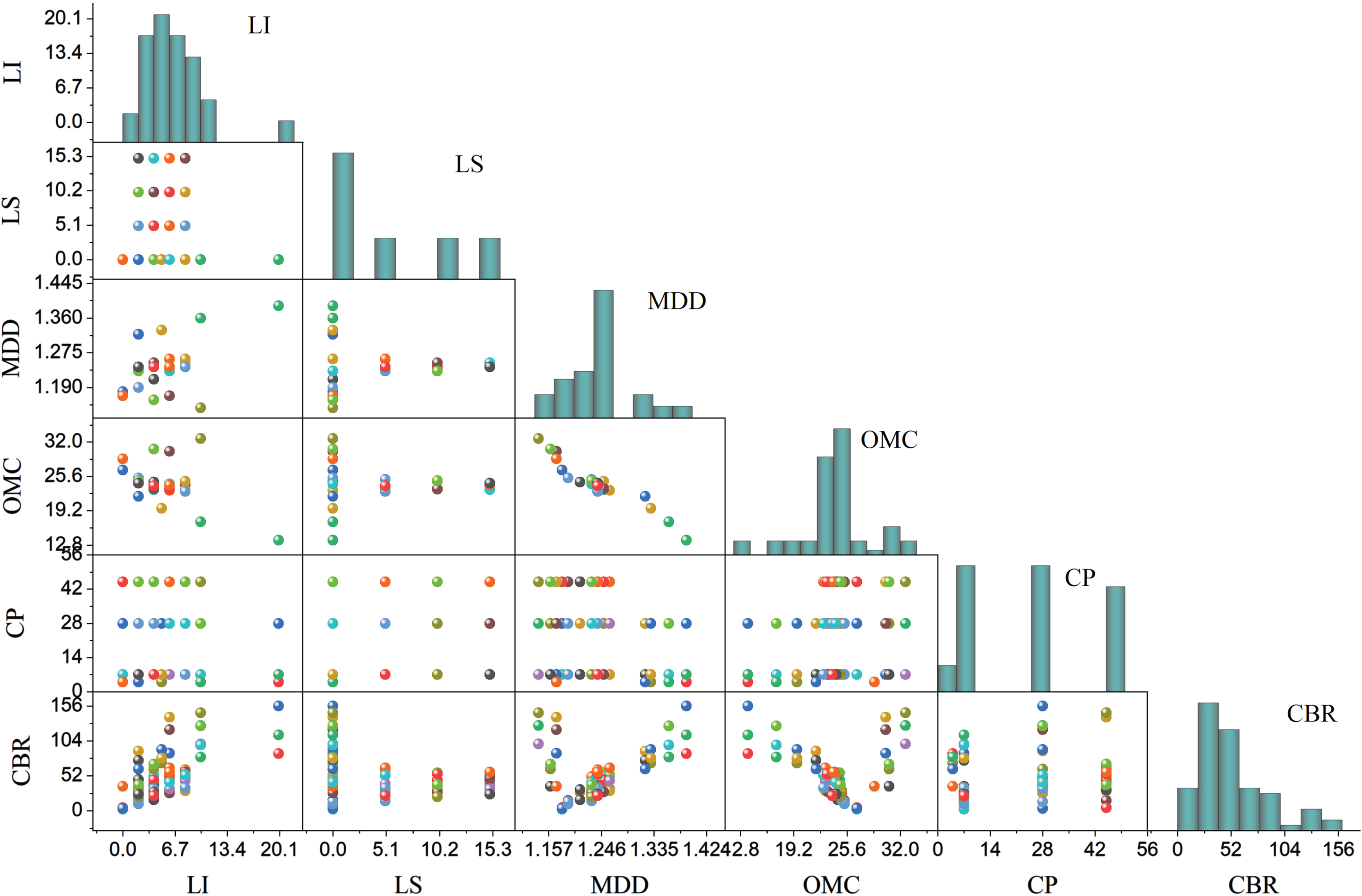
The scatter matric input and output variables.

2.2 Multi-layer perceptron (MLP)

The Multi-layer Perceptron (MLP) represents an extensively employed neural network architecture often trained through the backpropagation algorithm. MLPs are designed to handle learning and estimation processes, constituting a form of training and estimation art. These neural networks offer a versatile approach to approximating complex and nonlinear functions in real-world scenarios, showcasing their adaptability [26].

A single hidden layer within the MLP can proficiently model intricate functions thanks to its hidden neurons. A scarcity of neurons in this layer can result in suboptimal neural network performance. On the contrary, MLP neural networks can be intricate to train and susceptible to overfitting. The nodes in the output layer correspond to the number of variables being modeled.

To achieve the broad representation of the nonlinear function (l), the endeavor of function modeling involving a single predictor involves employing an MLP neural network, where X ∈ R ^D  → Y ∈ R¹. Here, Y and X denote the output and input parameters, respectively. The function (l) is mathematically expressed as shown in Equation (1):

$Y=l\left(X\right)=b_2+w_2\times \left(a\left(b_1+w_1\times X\right)\right)$(1)

w₁ and w₂ are the weights of hidden and outputlayers matrixes, respectively.

b₁ and b₂ show the hidden and output layers’ bias vectors, alternatively.

a shows the function of activation.

Equations (2) and (3) show the tan-sigmoid and log-sigmoid activation functions, alternatively:

$l\left(f\right)=\frac{1}{1+exp\left(-f\right)}$(2)

$l\left(f\right)=\frac{exp\left(f\right)-exp\left(-f\right)}{exp\left(f\right)+exp\left(-f\right)}$(3)

Here, f shows the function of input activation. Figure 2 shows the flowchart of MLP.

Fig. 2

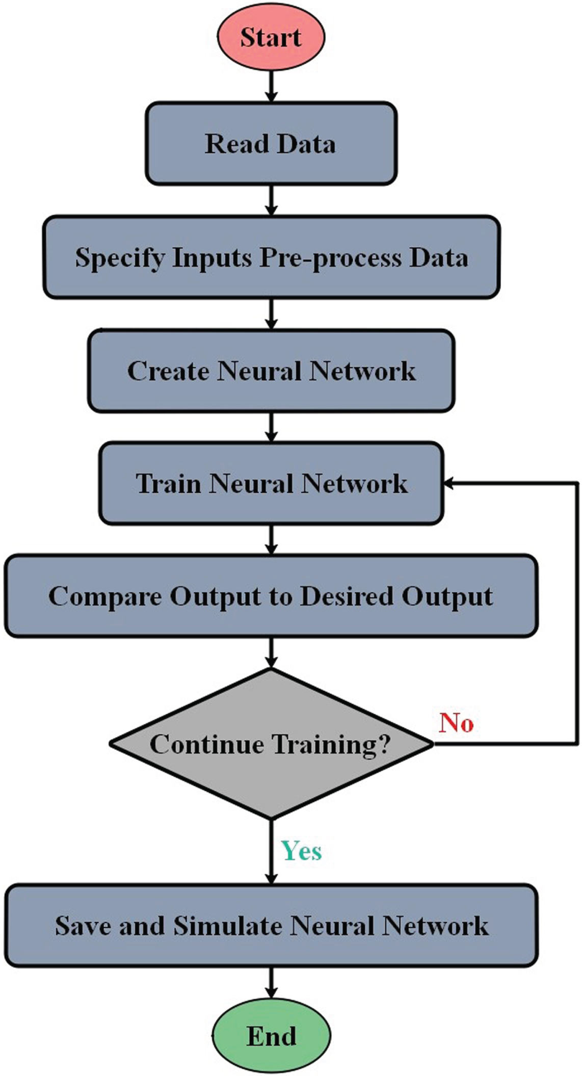
The flowchart of MLP.

2.3 MLP+BO

The Bonobo optimizer (BO) stands as a contemporary meta-heuristic algorithm, drawing inspiration from Bonobo primates’ reproducible behavior and social interactions. Das et al. [27] have formulated the BO algorithm in a population-based configuration.

The algorithm leverages natural behaviors by emulating bonobos’ optimal behavior and strategies. The BO incorporates four distinct mating strategies for generating new bonobo solutions: extra-group mating, promiscuous, restrictive, and consort ship [27]. These mating strategies may alter based on the circumstances’ phase, whether negative (NP) or positive (PP). The positive (PP) state reflects a bonobo community characterized by ample food resources, genetic diversity among bonobos, successful mating outcomes, and protection from external communities. Conversely, the NP phase denotes unfavorable conditions within the bonobo society.

2.3.1 Restrictive and promiscuous mating techniques

The phase probability parameter (m _m ) represents the Bonobo mating approach. Firstly, the amount of m _m is valued at 0.5, which is upgraded at each iteration. If a random number, q, is an amount from zero to one, a novel bonobo is produced. It is considered to be equal to or less than m _m as described in Equation (4):

$\begin{array}{cc}\hfill n_b{o}_j=& {\mathit{bo}}_j^i+q_1{t}^a\left(a_j^{\mathit{bo}}-{\mathit{bo}}_j^i\right)\hfill \\ \hfill & +\left(1-q_1\right)t^t\mathit{flag}\left({\mathit{bo}}_j^i-{\mathit{bo}}_j^m\right)\hfill \end{array}$(4)

Here bo stands for bonobo, n_bo_j and $a_j^{\mathit{bo}}$ are the j - th new offspring’ variables, j is a value that varies between 0 and 1, e is referred to the variables’ number, q₁ determines a random value within the range from 0 to 1, and t^a and t^t are referred to as sharing coefficients for a ^bo and m - th bonobos, respectively.

As the best response of i - th bonobo obtains a better consequence than m - th bonobos, promiscuous mating happens. In this situation, the flag is indicated 1. On the other hand, for limited mating a ^bo are assigned as –1.

2.3.2 Extra-group and consort ship mating techniques

If part m _m is lesser than q, these types of mating will happen. On the other hand, if q₂ is equal to or less than the extra group (m _xgm ) probability, this will result in upgrading the solution via extra-group mating.

$\{\begin{array}{c}{\mathit{bo}}_j^i+e^{\left(q_3^2+q_3-2q_3^{-1}\right)\left(\mathit{Va}{r}_{\mathit{ma}{x}_j}-{\mathit{bo}}_j^i\right){\alpha }_j^{\mathit{bo}}⩾{\mathit{bo}}_j^i}\hfill \\ {\mathit{bo}}_j^i-e^{\left(-q_4^2+2q_4-2q_4^{-1}\right)\left({\mathit{bo}}_j^i-\mathit{Va}{r}_{-\mathit{mi}{n}_j}\right)q_3⩽m_e}\hfill \\ {\mathit{bo}}_j^i-e^{\left(q_3^2+q_3-2q_3^{-1}\right)\left({\mathit{bo}}_j^i-\mathit{Va}{r}_{-\mathit{mi}{n}_j}\right){\alpha }_j^{\mathit{bo}}⩽{\mathit{bo}}_j^i}\hfill \\ {\mathit{bo}}_j^i+e^{\left(-q_4^2+2q_4-2q_4^{-1}\right)\left(\mathit{Va}{r}_{-\mathit{ma}{x}_j}-{\mathit{bo}}_j^i\right)q_3⩾m_e}\hfill \\ \hfill \end{array}$(5)

The m _e is started with 0.5 with an incremental upgrading related to the evolution’s nature, and itoptimizes the searching process for the foremost hopeful output. Var_{-min j} and Var_{-max j} denote the lowest and highest boundaries of the j - th variable, respectively.

In other cases, using the consortship mating strategy, a novel offspring is generated, where the amount of q₂ is found to be higher than that of m _xgm , as Equation (6):

$\begin{array}{cc}\hfill & n_b{o}_j=\hfill \\ \hfill & \{\begin{array}{c}{n}_b{o}_j+e^{q_5}\mathit{flag}\left(1+q_1\right)\left({\mathit{bo}}_j^i-{\mathit{bo}}_j^m\right)q_6⩽m_e\hfill \\ {\mathit{bo}}_j^m\mathit{otherwise}\hfill \\ \hfill \end{array}\hfill \end{array}$(6)

In these equations, q₁, q₂, q₃, q₄, q₅ are random numbers between 0 and 1.

The flowchart of the proposed algorithm is shown in Fig. 3.

Fig. 3

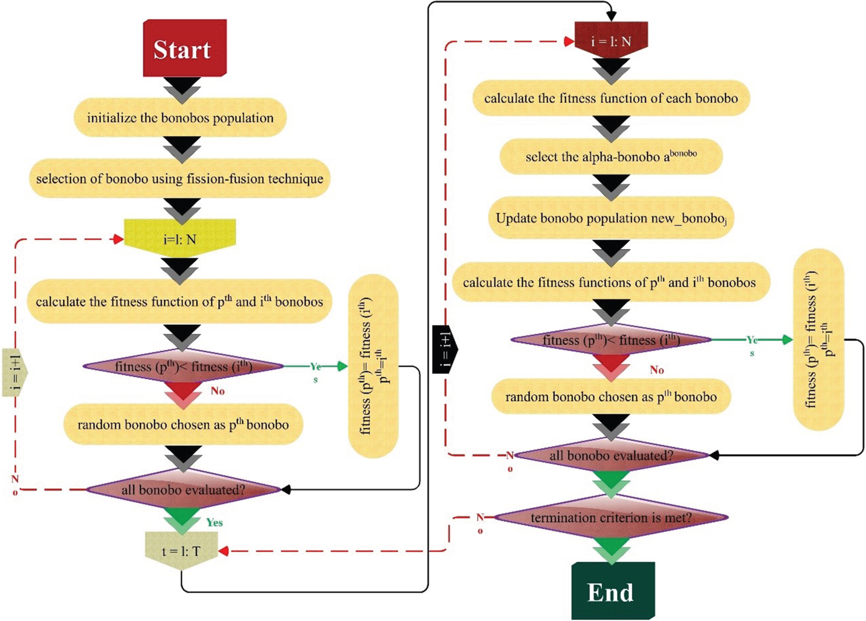
Bonobo structure.

2.4 MLP+SAO

The smelling sense is one of the initial senses through which the world is maintained. Most organisms sense the presence of harmful chemicals in their environment utilizing the smelling sense [28–30].

2.4.1 Sniffing mode

Because smell molecules spread in the agent’s direction, first start the process by arbitrarily developing smell molecules’ beginning location.

The smell molecules can be initialized using Equation (7):

$x_i^{\left(t\right)}=\left[\begin{array}{ccc}{x}_{\left(1,1\right)}\hfill & x_{\left(1,2\right)}\hfill & x_{\left(1,D\right)}\hfill \\ ·\hfill & ·\hfill & ·\hfill \\ x_{\left(N,1\right)}\hfill & x_{\left(N,2\right)}\hfill & x_{\left(N.D\right)}\hfill \\ \hfill & \hfill & \hfill \end{array}\right]$(7)

N is the total number of small molecules

D is the total number of decision variables.

The location vector in Equation (7) gives the agent the capability to identify its own best location in the space of search, and it can be obtained utilizing Equation (8):

$x_i^{\left(t\right)}=l{b}_i+r_0\times \left(u{b}_i-l{b}_i\right)$(8)

ub and lb indicate the upper and lower bound identified due to the decision variables, respectively

r₀ refers to a random value from 0 to 1.

Each smell molecule is assigned a primary velocity among that they spread from the smell source by utilizing Equation (9).

${\upsilon }_i^{\left(t\right)}=\left[\begin{array}{ccc}{\upsilon }_{\left(1,1\right)}\hfill & {\upsilon }_{\left(1,2\right)}\hfill & {\upsilon }_{\left(1,D\right)}\hfill \\ ·\hfill & ·\hfill & ·\hfill \\ {\upsilon }_{\left(N,1\right)}\hfill & {\upsilon }_{\left(N,1\right)}\hfill & {\upsilon }_{\left(N,D\right)}\hfill \\ \hfill & \hfill & \hfill \end{array}\right]$(9)

Each smell molecule indicates a candidate solution. The location of these candidate solutions is obtained from the position vector $x_i^{\left(t\right)}\in R^N$ represented in Equation (7) and the velocity of molecules ${\upsilon }_i^{\left(t\right)}\in R^N$ given in Equation (8). The molecules’ velocity is upgraded utilizing Equation (10).

$x_i^{t+1}=x_i^{\left(t\right)}+{\upsilon }_i^{t+1}\times \Delta t$(10)

Δt = 1 means that the agent progresses the path simultaneously through the optimization process. The new location of the smell molecules is calculated by Equation (11):

$x_i^{t+1}=x_i^{\left(t\right)}+{\upsilon }_i^{t+1}$(11)

Each smell molecule possesses diffusion velocities that can update and evaporate its location in search criteria. The updated smell velocity molecules are calculated employing Equation (12).

${\upsilon }_i^{t+1}={\upsilon }_i^{\left(t\right)}+\upsilon$(12)

υ is the update variable of the velocity derived by using Equation (13).

$\upsilon =r_1\times \sqrt{\frac{3\mathit{KT}}{m}}$(13)

k refers to the smell fixed that normalizes the influence of mass and temperature on the smell molecules’ kinetic energy.

m and T are the mass and temperature of the smell molecules, respectively.

The updated locations’ fitness of the smell molecule in Equation (11) is assessed. Thus, the sniffing mode is completed, and it is possible to determine the position of the agent $x_{\mathit{agent}}^t$ .

2.4.2 Trailing mode

In the second mode, the seeking behaviors of an agent are simulated to determine the origin of a smell. The agent may sniff a new location with a higher focus on smell molecules while searching for a smell source. By using Equation (14), the agent takes the opportunity towards this novel location:

$\begin{array}{cc}\hfill x_i^{t+1}=& x_i^{\left(t\right)}+r_2\times \mathit{olf}\times \left(x_{\mathit{agent}}^t-x_i^{\left(t\right)}\right)\hfill \\ \hfill & -r_3\times \mathit{olf}\times \left(x_{\mathit{worst}}^t-x_i^{\left(t\right)}\right)\hfill \end{array}$(14)

r₂ and r₃ are numbers from 0 to 1

r2 penalizes the influence of olf on $x_{\mathit{agent}}^t$ and r₃ penalizes the effect of the olf on $x_{\mathit{worst}}^t$ .

The agent records $x_{\mathit{agent}}^t$ and the $x_{\mathit{worst}}^t$ gained from the sniffing mode.

2.4.3 Random mode

If large distances segment the molecules of smell, the intensity of the smell molecule might be different over the period. This difference may “bemuse” the agent, results in the smell’s loss, and makes trailing a significant challenge. Due to its disability to preserve trailing, the agent might be caught in local minima. If this happens, the agent transfers to the random mode, which is represented using Equation (15):

$x_i^{t+1}=x_i^{\left(t\right)}+r_4\times \mathit{SL}$(15)

SL is the step length.

r4 is a random value that penalizes the amount of SL.

The pseudo-code of the SAO algorithm is given in Algorithm 1, and the flowchart of SAO is indicated in Fig. 4.

Fig. 4

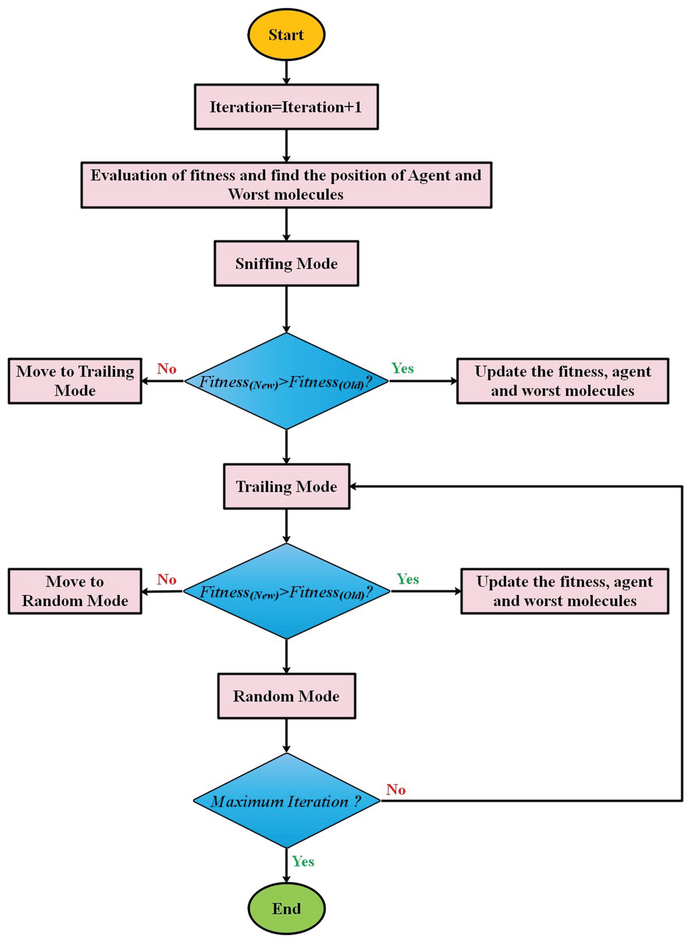
The flowchart of SAO.

Algorithm 1: Smell Agent Optimization

Initialize Parameters

Initialize smell molecules’ initial position

Assess fitness

Prepare the location of the agent and the worst position of molecules

While (Itr < Itr max ) do:

for (i = 1 to molecules) do:

for (j = 1 to position) do:

update molecules’ velocity and position (sniffing)

end for

Assess fitness

if (new fitness is better) then:

Update fitness

Update agent and worst molecules

end if

end for

for (i = 1 to molecules) do:

for (j = 1 to position) do:

update position (trailing)

end for

Assess fitness

end for

if (new fitness is better) then:

grant new fitness

update position

else

for (i = 1 to molecules) do:

for (j = 1 to position) do:

Implement random mode

end for

end for

end if

end while

return optimum solution.

2.5 MLP+PDO

2.5.1 Initialize

Each Prairie Dog (P) in a clique (nP) is a member of k other cliques. PD operates and behaves in groups or cliques. Thus, a vector can be used to determine the location of the ith prairie dog within a specific clique. The location of each Coterie (S) within the territory is described by Equation (16):

$S=\left[\begin{array}{ccccc}{S}_{1,1}\hfill & S_{1,2}\hfill & \dots \hfill & S_{1,D-1}\hfill & S_{1,D}\hfill \\ ⋮\hfill & ⋮\hfill & S_{i,j}\hfill & ⋮\hfill & ⋮\hfill \\ S_{k,1}\hfill & S_{k,2}\hfill & \dots \hfill & S_{k,D}\hfill & S_{k,D}\hfill \\ \hfill & \hfill & \hfill & \hfill & \hfill \end{array}\right]$(16)

Here S_i,j is the dimension of jth of the Coterie of ith in a territory. Each prairie dog in a coterie has a position in Equation (17).

$\mathrm{P}=\left[\begin{array}{ccccc}{P}_{1,1}\hfill & P_{1,2}\hfill & \dots \hfill & P_{1,D-1}\hfill & P_{1,D}\hfill \\ ⋮\hfill & ⋮\hfill & P_{i,j}\hfill & ⋮\hfill & ⋮\hfill \\ P_{k,1}\hfill & P_{k,2}\hfill & \dots \hfill & P_{k,D}\hfill & P_{k,D}\hfill \\ \hfill & \hfill & \hfill & \hfill & \hfill \end{array}\right]$(17)

Here P_i,j is the dimension of jth of the Coterie of ith in a territory and n ⩽ k. Using a distribution of uniforms as in Equations (18) and (19), respectively, the positions of each clique and prairie dog are determined.

$S_{i,j}=u\left(0,1\right)\times \left(u{b}_j-l{b}_j\right)+l{b}_j$(18)

$P_{i,j}=u\left(0,1\right)\times \left(u{b}_j-l{b}_j\right)+l{b}_j$(19)

Here lb _j and ub _j show the lower and upper bounds of the dimension jth of the optimization issue and u(0,1) shows a random number with a distribution of uniform between 0 and 1.

2.5.2 Fitness function evaluation

The fitness function values for each position of the prairie dog were determined by providing the solution vector to the fitness function definition. The values that result are saved in a collection that looks like this:

$f\left(P\right)=\left[\begin{array}{ccccc}{f}_1(P_{1,1}\hfill & P_{1,2}\hfill & \dots \hfill & P_{1,D-1}\hfill & P_{1,D})\hfill \\ ⋮\hfill & ⋮\hfill & P_{i,j}\hfill & ⋮\hfill & ⋮\hfill \\ f_n(P_{k,1}\hfill & P_{k,2}\hfill & \dots \hfill & P_{k,D}\hfill & P_{k,D})\hfill \\ \hfill & \hfill & \hfill & \hfill & \hfill \end{array}\right]$(20)

2.5.3 Search

PD0 is capable of switching between exploitation and search based on four positions. Divide the maximum number of iterations by 4. While the last two parts are used for development, the first is used for search. The two processes employed for search depend on 4 $\mathit{iter}<\frac{\mathit{Ma}{x}_{\mathit{It}}}{4}$ and $\frac{\mathit{Ma}{x}_{\mathit{It}}}{2}⩽\mathit{iter}<\frac{\mathit{Ma}{x}_{\mathit{It}}}{4}$ , while the two processes used for development depend on $\frac{\mathit{Ma}{x}_{\mathit{It}}}{2}⩽\mathit{iter}<3\frac{\mathit{Ma}{x}_{\mathit{It}}}{4}$ and $3\frac{\mathit{Ma}{x}_{\mathit{It}}}{4}⩽\mathit{iter}<\mathit{Ma}{x}_{\mathit{It}}$ .

During the search phase, the first procedure is to have faction members scour the neighborhood for fresh food sources, as shown in Fig. 5. Equation (21) gives the foraging position update during our algorithm’s search phase. The statue aids in controlling the growth of the caves. Equation (22) provides this location update for the construction of caves.

Fig. 5

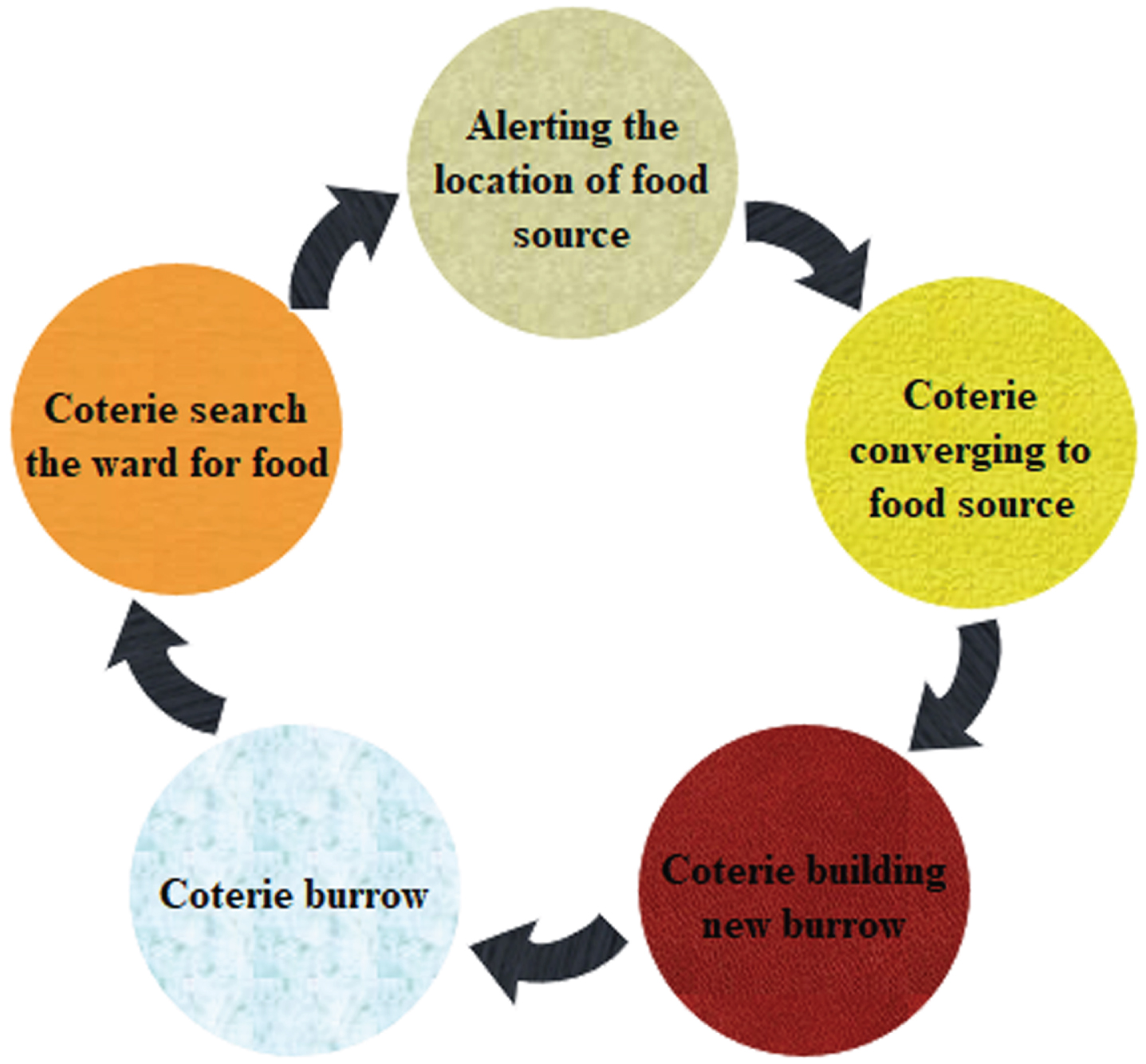
Search section’s model.

$\begin{array}{cc}\hfill P_{i+1,j+1}=& \mathit{OBes}{t}_{i,j}-\mathit{eEBes}{t}_{i,j}\times a-E{P}_{i,j}\hfill \\ \hfill & \times \mathit{Levy}\left(n\right)\mathit{for}\mathit{iter}<\frac{\mathit{Ma}{x}_{\mathit{It}}}{4}\hfill \end{array}$(21)

$\begin{array}{cc}\hfill P_{i+1,j+1}=& \mathit{OBes}{t}_{i,j}\times r-C\times \mathit{Levy}\left(n\right)\hfill \\ \hfill & \mathit{for}\frac{\mathit{Ma}{x}_{\mathit{It}}}{2}⩽\mathit{iter}<\frac{\mathit{Ma}{x}_{\mathit{It}}}{4}\hfill \end{array}$(22)

Here OBest_i,j shows the overall best solution obtained so far, and eEBest_i,j assess the current’s effect to achieve the best solution as in Equation (23), shows a particular food source alarm. r indicates the random solution location and EP_i,j determines the randomized cumulative all prairie dogs’ effect within the colony and is given by Equation (24). C is the creek digging intensity, which relies on the food source’s quality and takes a random value given by Equation (23). Levy (n) is the distribution of Levy (n), known to promote suitable and more efficient search of the problem exploration space [31]:

$\begin{array}{cc}\hfill \mathit{eEBes}{t}_{i,j}=& \mathit{OBes}{t}_{i,j}\times A\hfill \\ \hfill & +\frac{P_{i,j}\times \mathit{mean}\left(P_{n,k}\right)}{\mathit{OBes}{t}_{i,j}\times u{b}_j-l{b}_j+A}\hfill \end{array}$(23)

$E{O}_{i,j}=\frac{\mathit{OBes}{t}_{i,j}\times r}{\mathit{OBes}{t}_{i,j}+A}$(24)

$C=1.5\times s\times {\left(1-\frac{\mathit{iter}}{\mathit{Ma}{x}_{\mathit{It}}}\right)}^{\left(2\frac{\mathit{iter}}{\mathit{Ma}{x}_{\mathit{It}}}\right)}$(25)

Here s is a probabilistic property that ensures the search, taking values of ndash 1 or 1 relying on the iteration of current, respecting between ndash 1 and 1 if the current iteration is even or odd. However, the PDO application considered they were all the same. iter shows the current iteration, and Max _It indicates the iterations’ maximum number.

2.5.4 Exploitation

Specific responses to two unique communications or alarm sounds in prairie dogs are employed to achieve exploitation in the suggested PDO, as indicated in Fig. 6. Equations (26) and (27) give the two processes envisioned in this section. As already mentioned, PDOmoves between these two processes depending on $\frac{\mathit{Ma}{x}_{\mathit{It}}}{2}⩽\mathit{iter}<3\frac{\mathit{Ma}{x}_{\mathit{It}}}{4}$ and $3\frac{\mathit{Ma}{x}_{\mathit{It}}}{4}⩽\mathit{iter}<\mathit{Ma}{x}_{\mathit{It}}$ , alternatively.

Fig. 6

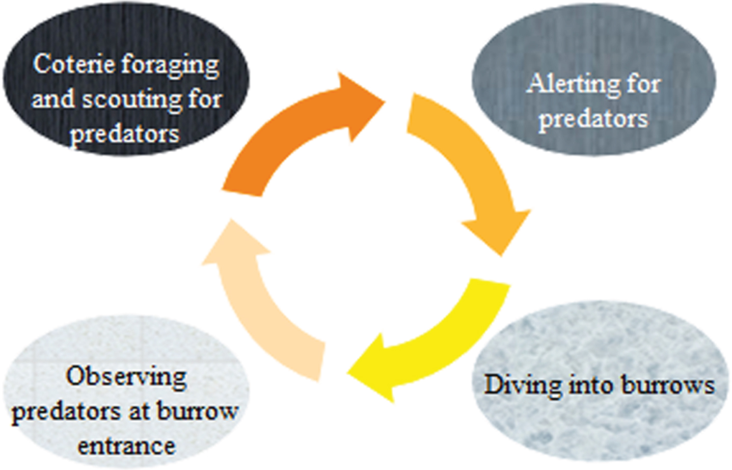
Exploitation’s model.

$\begin{array}{cc}\hfill P_{i+1,j+1}=& \mathit{OBes}{t}_{i,j}-\mathit{eEBes}{t}_{i,j}\times q-E{P}_{i,j}\hfill \\ \hfill & \times \mathit{rand}\mathit{for}\frac{\mathit{Ma}{x}_{\mathit{It}}}{2}⩽\mathit{iter}<3\frac{\mathit{Ma}{x}_{\mathit{It}}}{4}\hfill \end{array}$(26)

$\begin{array}{cc}\hfill P_{i+1,j+1}=& \mathit{OBes}{t}_{i,j}\times F\times \mathit{rand}\mathit{for}3\frac{\mathit{Ma}{x}_{\mathit{It}}}{4}\hfill \\ \hfill & ⩽\mathit{iter}<\mathit{Ma}{x}_{\mathit{It}}\hfill \end{array}$(27)

$F=1.5\times {\left(1-\frac{\mathit{iter}}{\mathit{Ma}{x}_{\mathit{It}}}\right)}^{\left(2\frac{\mathit{iter}}{\mathit{Ma}{x}_{\mathit{It}}}\right)}$(28)

A small variety defining the high satisfaction of the food supply is shown in q, and the impact of the predator is shown in s. Additionally, Algorithm 2 presents the PDO pseudo-code.

Algorithm 2. Prairie Dog Optimizer pseudo-code

Initialization

Set the PDO parameter: n,k,a,q

Set GBest and EBest

Initialization of the candidate solution S and P

Whileiter < Max It do

For (i = 1 to k)do

For (j = 1 to k)do

Compute the P’s fitness

Find the Best solution so far (EBest)

Update OBest

Update C and F

Update EPi,j

If $\left(\mathit{iter}<\frac{\mathit{Ma}{x}_{\mathit{It}}}{4}\right)$ then using

Else if $\left(\frac{\mathit{Ma}{x}_{\mathit{It}}}{2}⩽\mathit{iter}<\frac{\mathit{Ma}{x}_{\mathit{It}}}{4}\right)$ then using

Else if $\left(\frac{\mathit{Ma}{x}_{\mathit{It}}}{2}⩽\mathit{iter}<3\frac{\mathit{Ma}{x}_{\mathit{It}}}{4}\right)$ then using

Else using Equation (16)

End If

End For

End For

iter = iter + 1

End While

Return thebest solution (OBest)

End

The flowchart of PDO is shown in Fig. 7.

Fig. 7

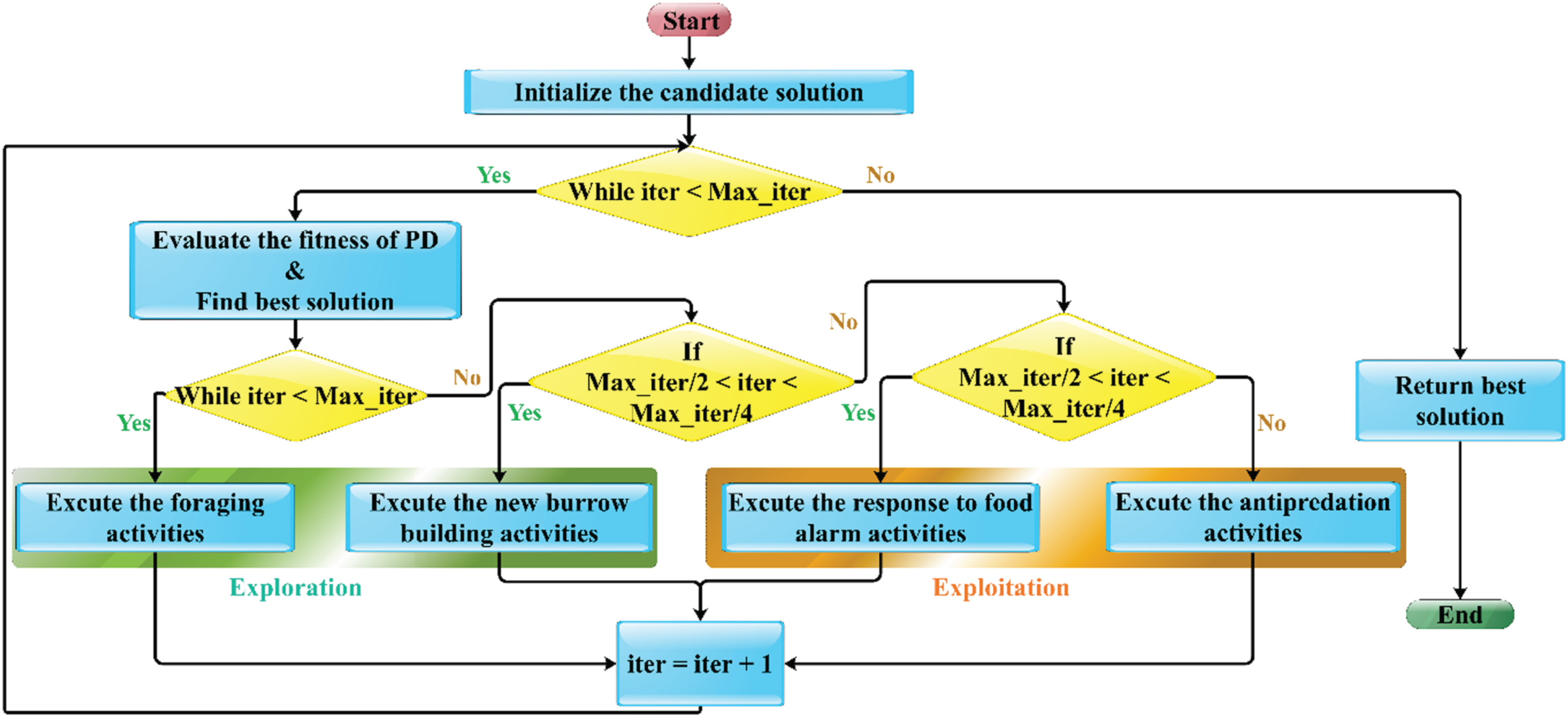
The flowchart of the PDO algorithm.

2.6 MLP+GRO

The GRO algorithm was developed by utilizing the potential of human reasoning and decision-making to locate the gold. A team of operators is dispersed randomly throughout the search area to start the search. Each operator watches for devices that produce a louder sound and listens for sounds produced by other equipment while paying attention to their own [32]. The GRO algorithm’s flowchart can be found in Fig. 8.

Fig. 8

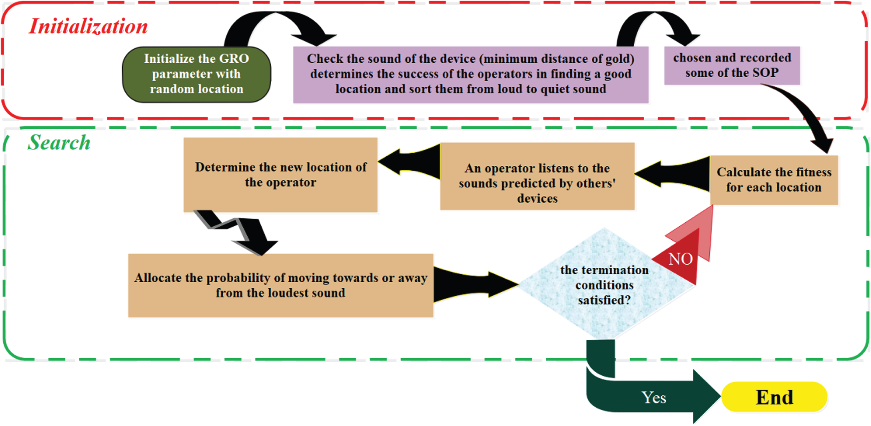
The flowchart of the GRO algorithm.

2.6.1 First step: initialization

Equation (29) represents the random assignment of a location to each operator within the search area. Rand denotes a random number within the range of [0, 1], and the search spaces for the operators are defined by ub _i and lb _i .

$\begin{array}{cc}\hfill {\mathit{location}}_t^{\left(0\right)}=& l{b}_i+\left(u{b}_i-l{b}_i\right)\times \mathit{rand},\hfill \\ \hfill & i=1,2,\dots ,n\hfill \end{array}$(29)

2.6.2 Second step: Monitoring, refers to the process of selecting optimal locations

An operator who successfully locates the ideal location is known as the SOP. After each iteration, it is advised to keep the top 10% of operators in the SOP.

2.6.3 Third step: Fitness-distance, refers to the relationship between fitness and distance

Using Equation (30), the loudness of each sound (rate) is calculated to identify the operator with the best chance of finding gold.

$\mathit{rate}\left(i\right)=\frac{D_i}{P_i}\times \frac{\mathit{sound}\left(\mathit{highest}\mathit{volume}\right)-\mathit{sound}\left(i\right)}{\left(\mathit{sound}\left(\mathit{highest}\mathit{volume}\right)-\mathit{sound}\left(\mathit{lowest}\mathit{volume}\right)+\varepsilon \right)}$(30)

To mitigate environmental errors, the coefficients in Equations (31-32) are utilized, represented by D _i and P _i , respectively.

$D_i=\sqrt{{\left(x_i-x_j\right)}^2+{\left(y_i-y_j\right)}^2+}$(31)

$P_i=2-\frac{\mathit{ite}}{\mathit{ma}{x}_{\mathit{ite}}}$(32)

At this point, based on a variety of sounds, each operator makes a unique decision. Equation (32) is a representation of this procedure.

$\begin{array}{cc}\hfill & \mathit{new}\mathit{location}\left(i\right)=\mathit{location}\left(i\right)+\mathit{md}\times \hfill \\ \hfill & [\left(\mathit{rate}\left(j\right)-\mathit{rate}\left(i\right)\right)\times \left(\mathit{location}\left(j\right)-\mathit{location}\left(i\right)\right)\hfill \\ \hfill & \times \mathit{rand}]\hfill \end{array}$(33)

The MD coefficients, which are specified in Equation (34), represent the direction of movement:

$\begin{array}{cc}\hfill & \mathit{md}=\hfill \\ \hfill & \{\begin{array}{c}+1\Rightarrow \mathit{towards}a\mathit{loudest}\mathit{sound}a>\mathit{rand}\hfill \\ -1\Rightarrow \mathit{away}\mathit{from}a\mathit{loudest}\mathit{sound}a<\mathit{rand}\hfill \\ \hfill \end{array}\hfill \end{array}$(34)

2.6.4 Fourth step: Location correction

The coefficients β and γ are selected from the range of 0 < β < γ < 1if Equation (35) fails to provide a satisfactory location, and Equation (35) is used to generate new locations.

$\begin{array}{cc}\hfill & \mathit{new}\mathit{location}\left(i\right)=\hfill \\ \hfill & \{\begin{array}{cc}\mathit{choose}a\mathit{neighboring}\mathit{location}\hfill & \mathit{rand}<\beta \hfill \\ \mathit{select}a\mathit{new}\mathit{location}\mathit{randomly}\hfill & \beta <\mathit{rand}<\gamma \hfill \\ \mathit{do}\mathit{not}\mathit{move}\hfill & \gamma <\mathit{rand}\hfill \\ \hfill & \hfill \end{array}\hfill \end{array}$(35)

Iterative Termination: The four termination steps, labeled as steps 1through 4, constitute a cyclic process that continues until the fulfillment of any of the subsequent conditions:

2.7 Performance evaluation methods

Different evaluators were exploited to assess the application of hybrid models to predict the value of the CBR. Coefficient of determination (R²), root mean squared error (RMSE), Mean squared error (MSE), Median Absolute Percentage Error (MDAPE), and Weighted Absolute Percentage Error (WAPE). The coefficient R² determines the linear correlation degree between the actual and predicted amounts. RMSE indicates the square root of the ratio of the estimated value deviation from the actual value to the square of the number of specimens. The WAPE is equal to the sum of the absolute error divided by the sum of the actual demand.

The values of these metrics mentioned above are provided by Equations (36–40).

$R^2=\left(\frac{{\sum }_{i=1}^n\left(b_i-\overline{b}\right)\left(d_i-\overline{d}\right)}{\sqrt{\left[{\sum }_{i=1}^n{\left(b_i-\overline{d}\right)}^2\right]}\left[{\sum }_{i=1}^n{\left(d_i-\overline{d}\right)}^2\right]}\right)$(36)

$\mathit{RMSE}=\sqrt{\frac{1}{n}\sum _{i=1}^n{\left(d_i-p_i\right)}^2}$(37)

$\mathit{MSE}=\frac{1}{n}\sum _{i=1}^n\left({\left(d_i-p_i\right)}^2\right)$(38)

$\mathit{MDAPE}=\mathit{median}\left(\frac{1}{n}\sum _{i=1}^n\left|\frac{d_i-b_i}{d_i}\right|\times 100\%\right)$(39)

$\mathit{WAPE}=\frac{{\sum }_{i=1}^n\left|d_i-b_i\right|}{{\sum }_{i=1}^n\left|b_i\right|}$(40)

n shows the numbers related to the samples, d _i shows the predicted value, b _i indicates the experimental value, $\overline{d}$ refers to the meanof the predicted value and $\overline{b}$ is the mean of the experimental amount.

2.8 Hyperparameter

Table 2 presents the hyperparameters for the developed models, explicitly detailing the structure in terms of layers and the number of neurons within each layer. The models listed are MLSA, MLBO, MLPD, and MLGR.

Table 2

The hyperparameters of developed models

Layer	Model	Index values
		Neuron	Neuron	Neuron
First	MLSA	13	–	–
	MLBO	7	–	–
	MLPD	12	–	–
	MLGR	9	–	–
Second	MLSA	12	4	–
	MLBO	26	19	–
	MLPD	3	6	–
	MLGR	5	9	–
Third	MLSA	6	11	16
	MLBO	6	18	18
	MLPD	21	21	9
	MLGR	12	16	17

–In the first layer, the MLSA, MLBO, MLPD, and MLGR models have 13, 7, 12, and 9 neurons, respectively.

–In the second layer, the models have varying numbers of neurons for each of the four models: MLSA has 12, 4, and an empty cell denoting no neuron count; MLBO has 26, 19, and an empty cell; MLPD has 3, 6, and an empty cell; and MLGR has 5, 9, and an empty cell.

–In the third layer, the models have further varying numbers of neurons: MLSA has 6, 11, and 16 neurons; MLBO has 6, 18, and 18 neurons; MLPD has 21, 21, and 9 neurons; and MLGR has 12, 16, and 17 neurons.

The table essentially provides an overview of the model architecture, illustrating the arrangement of layers and the number of neurons within each layer for the mentioned models.

3 Results and discussion

3.1 Comparison of developed models

In this study, we have developed three distinct hybrid models for predicting the California bearing ratio by combining the Multi-Layer Perceptron (MLP) with the BO and SAO, PDO, and GRO algorithms. These hybrid models utilize a data division into a training set (70%) and a test set (30%) to assess their performance. This section involves a comparative analysis of statistical indicators associated with these developed models to ascertain any superiority of one version over the others.

Tables 3 to 5 present the results of applied ML models for CBR in different layers (1, 2, and 3). The models evaluated are MLSA, MLBO, MLPD, and MLGR. The evaluation is conducted during training and testing phases, with critical indices including RMSE, R², MSE, MAPE, and SI recorded for each phase.

Table 3

The result of developed models for CBR in layer (1)

Model	Phase	Index values
		RMSE	R2	MSE	MAPE	SI
MLSA	Train	5.385	0.978	28.997	8.354	0.099
	Test	6.519	0.966	42.495	6.603	0.132
	All	5.750	0.973	33.065	7.826	0.109
MLBO	Train	7.445	0.960	55.429	62.927	0.137
	Test	6.200	0.951	38.435	13.629	0.125
	All	7.093	0.957	50.307	48.070	0.134
MLPD	Train	4.300	0.988	18.489	6.659	0.079
	Test	2.362	0.993	5.580	2.139	0.048
	All	3.821	0.988	14.598	5.297	0.072
MLGR	Train	5.251	0.980	27.576	9.515	0.096
	Test	2.993	0.992	8.960	6.478	0.061
	All	4.687	0.982	21.966	8.600	0.088

Table 4

The result of developed models for CBR in layer (2)

Model	Phase	Index values
		RMSE	R2	MSE	MAPE	SI
MLSA	Train	4.819	0.985	23.223	9.551	0.088
	Test	4.147	0.980	17.194	7.799	0.084
	All	4.627	0.984	21.406	9.023	0.087
MLBO	Train	6.708	0.966	44.999	18.499	0.123
	Test	6.491	0.953	42.130	15.287	0.131
	All	6.643	0.963	44.134	17.531	0.125
MLPD	Train	5.093	0.981	25.937	8.756	0.093
	Test	4.022	0.981	16.173	8.404	0.081
	All	4.795	0.981	22.994	8.650	0.091
MLGR	Train	5.481	0.978	30.041	5.115	0.101
	Test	3.084	0.989	9.513	3.870	0.062
	All	4.884	0.980	23.854	4.740	0.092

Table 5

The result of developed models for CBR in layer (3)

Model	Phase	Index values
		RMSE	R2	MSE	MAPE	SI
MLSA	Train	2.800	0.994	7.842	4.199	0.051
	Test	2.878	0.990	8.282	3.118	0.058
	All	2.824	0.993	7.975	3.873	0.053
MLBO	Train	5.728	0.978	32.813	11.358	0.105
	Test	5.195	0.969	26.986	7.674	0.105
	All	5.573	0.976	31.057	10.248	0.105
MLPD	Train	4.679	0.984	21.897	8.207	0.086
	Test	8.677	0.970	75.291	11.364	0.175
	All	6.163	0.971	37.988	9.158	0.116
MLGR	Train	3.088	0.993	9.534	6.707	0.057
	Test	6.107	0.954	37.295	11.445	0.124
	All	4.231	0.985	17.900	8.135	0.080

In Table 3, which focuses on Layer 1, the models demonstrate varying performance across the phases. MLSA exhibits a low RMSE during training, indicating good predictive accuracy. MLBO, though presenting higher RMSE and MAPE, maintains competitive R² values. MLPD stands out for its notably low RMSE and MAPE in the testing phase. MLGR shows solid performance in both the training and testing phases.

Table 4, for Layer 2, continues to reveal variations in model performance. MLSA showcases consistent and robust performance across phases. MLBO, while experiencing higher RMSE and MAPE, maintains competitive R² values. MLPD displays a good balance of RMSE and MAPE in the testing phase. MLGR performs exceptionally well in the testing phase with low RMSE and MAPE.

Finally, Table 5 delves into Layer 3, unveiling further nuances in model performance. MLSA maintains its strong performance, with low RMSE and high R² values. MLBO shows slightly increased RMSE and MAPE in the testing phase but maintains competitive performance. MLPD, despite a higher RMSE in testing, remains competitive across all phases. MLGR demonstrates excellent performance in training and holds a relatively higher RMSE in the testing phase.

In summary, these tables provide a comprehensive view of how different ML models predict CBR across various layers, showcasing their strengths and areas for improvement. The results offer valuable insights for optimizing model selection and performance across different evaluation phases. In addition, Fig. 9 indicates R², RMSE, and MSE comparisons between the developed models.

Fig. 9

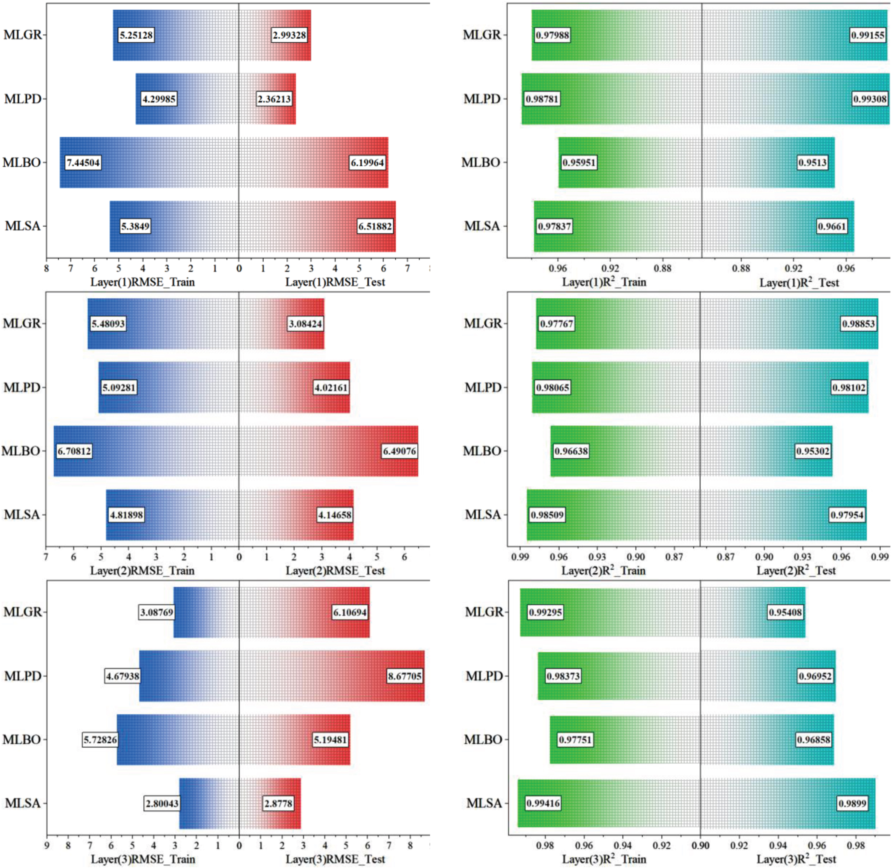
The comparison of metrics between layers.

The study illustrates the correlation between predicted and measured CBR models through stacked columns and scatter plots presented in Fig. 10, categorized into training and testing. These categories provide a comprehensive contrast for the predictions of the top-performing hybrid models, namely MLPD (layer 1), MLSA (layer 2), and MLSA (layer 3). The research findings underscore the impressive predictive accuracy of these models, revealing a robust positive correlation between expected and observed values. Notably, MLSA in layer 3 stands out as exceptionally superior due to its precise clustering of data points along linear regression lines. This model consistently exhibits minimal variation across all stages compared to the frequently higher measured values. Comparatively, the linear regression lines for MLPD in layer 1 and MLSA in layer 2 models display similar slope and intercept values, indicating equivalent prediction capabilities. However, MLPD (layer 1) and MLSA (layer 2) exhibit slightly greater dispersion among their data points. While their predicted points deviate slightly from the measured values, they still demonstrate respectable accuracy, albeit not as exceptional as MLSA in layer 3.

Fig. 10

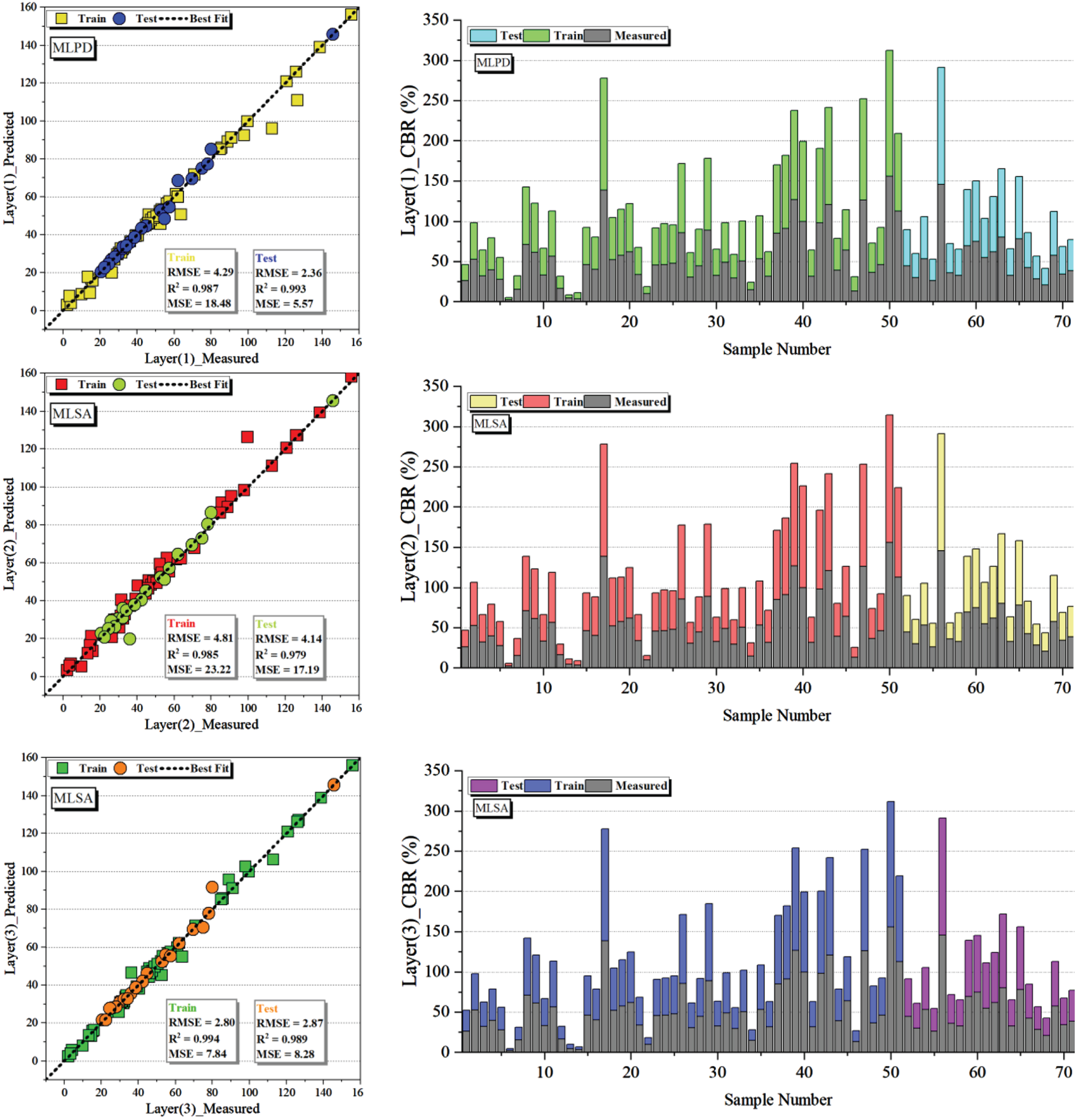
The stacked column and scatter plot of the correlation between the predicted and measured CBR models.

The study employs visual representations, specifically histograms and line plots in Fig. 11, to illustrate the error rate percentages for the hybrid models. Notably, most samples exhibit a high degree of consistency, tightly clustered within a relatively narrow error range of –15% to 15%. However, there is an outlier in the MLSA model in layer (3), which reaches as high as 30%. Among the three models under examination, the MLPD model in layer (1) stands out due to its more comprehensive range of error percentages, spanning from –20% to 20%, with a notable outlier at 120%. In contrast to the other two models, this broader range indicates increased variability and a lower level of predictive precision. On the other hand, the MLSA model in layer (2) distinguishes itself by displaying a wider range of error percentages, ranging from –19% to 19%, with an outlier at 65%.

Fig. 11

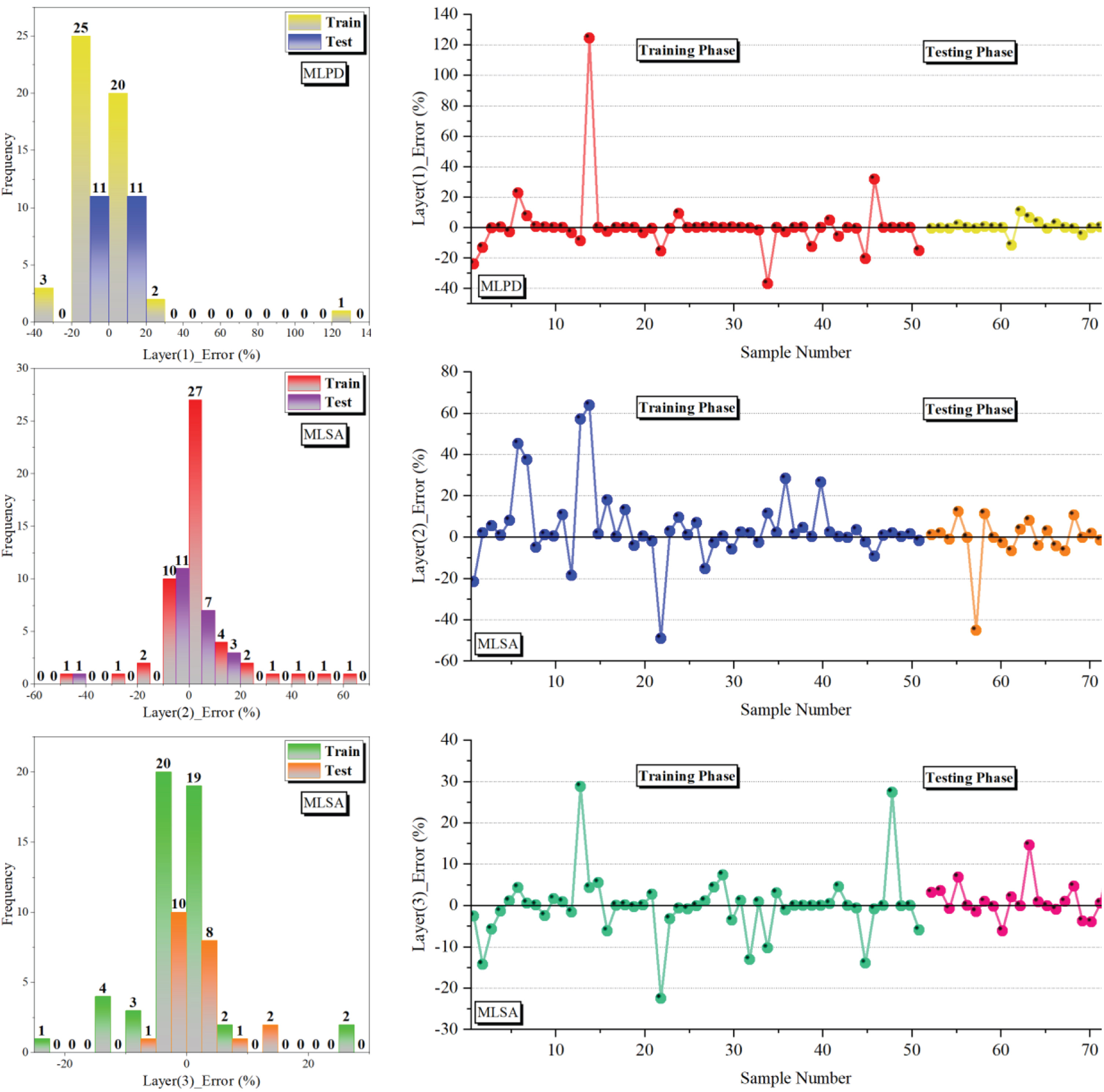
The error percentage of presented models is based on a line-symbol plot and histogram for CBR.

Figure 12 presents a box plot illustrating error percentages associated with three distinct models. Notably, the MLSA model in layer (3) emerges as a standout performer, consistently showcasing errors within the narrow range of –5% to 5% during the training and testing phases, displaying minimal variability. Conversely, the MLPD model in layer (1) exhibits error dispersion across both phases, manifesting a uniform normal distribution of errors that do not exceed the range of –20% to 20%. It is worth emphasizing that the Gaussian distribution observed in the MLPD model in layer (1) and the MLSA model in layer (2) signifies increased dispersion, accompanied by a diminished frequency of occurrences near 0%.

Fig. 12

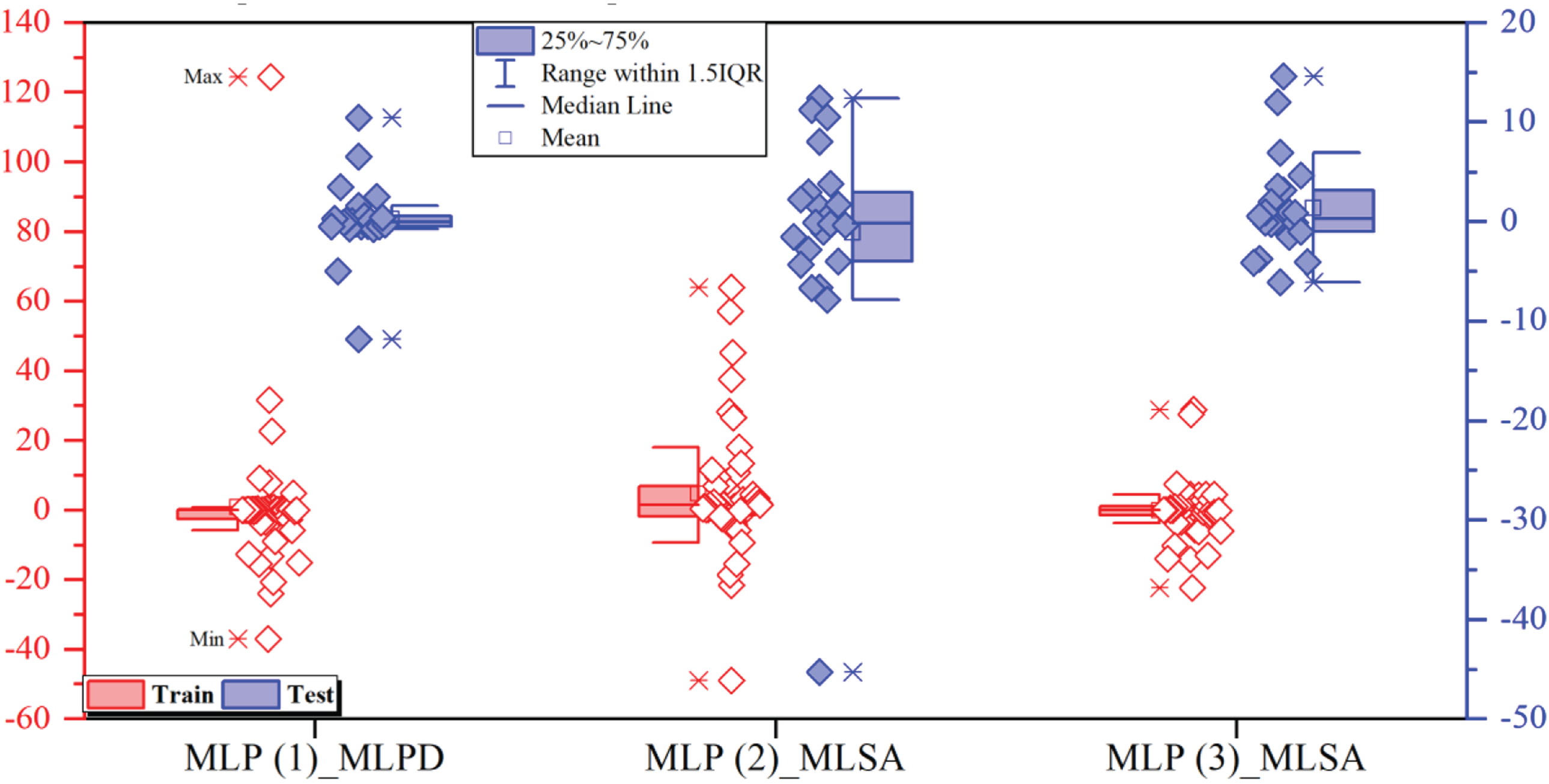
The box for the error percentage of the developed models for CBR.

3.2 Sensitivity analysis

3.2.1 Cosine amplitude method (CAM)

Academic Rephrase: Sensitivity analysis employing cosine amplitude refers to a method, either analytical or computational, that entails assessing the sensitivity of a system or model by utilizing cosine amplitudes or cosine functions. Figure 13 provides the outcomes of sensitivity analysis for input parameters LI, LS, MDD, OMC, and CP. The sensitivity indices elucidate the impact of each parameter on the model’s output, wherein higher values signify a more notable influence. Notably, LS does not exert any influence, whereas the remaining parameters exhibit varying degrees of influence. The accompanying confidence intervals quantify the uncertainty surrounding these sensitivity indices, contributing to a comprehensive grasp of the model’s responsiveness to alterations in input. These insights are pivotal for making informed decisions and refining the model effectively.

Fig. 13

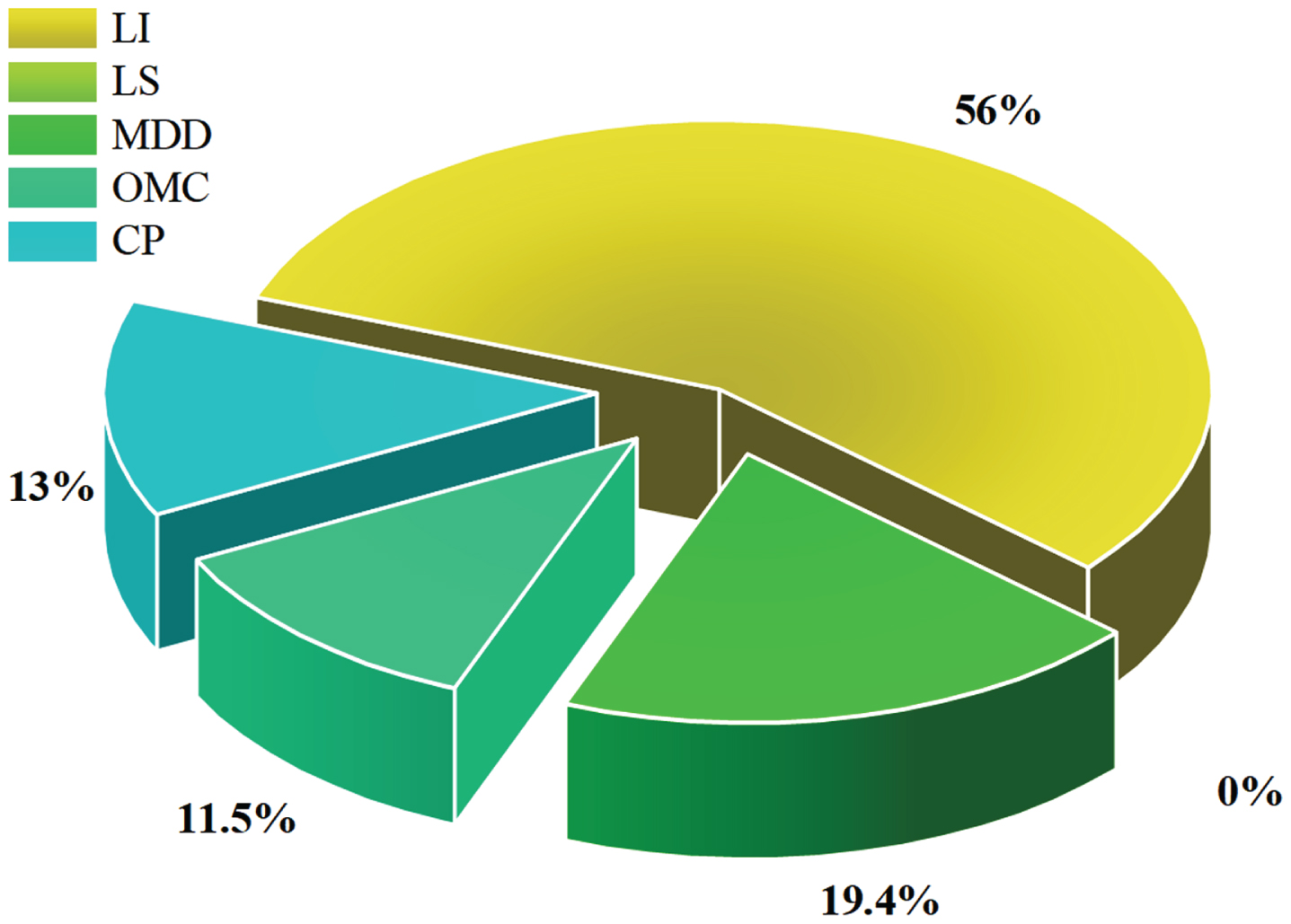
The sensitivity of each input on output.

4 Conclusion

The current study conducted an AI procedure to predict the mechanical properties of the pond ash’s California Bearing Ratio (CBR) value justified with lime sludge and lime. Nevertheless, the values obtained from the traditional method were accurate but had some disadvantages. The laboratory method is not only cost-effective in terms of time, but also it requires high costs. Artificial intelligence (AI) replaces the software method to solve these weaknesses. The system can predict the CBR precisely. For this purpose, multi-layer perceptron (MLP) produces powerful compound models consisting of Bonobo Optimizer (BO), Prairie dog optimization (PDO), Gold Rush Optimizer (GRO), and Smell Agent Optimization (SAO) for soil’s CBR value prediction. According to the results, it can be concluded as follows:

In Layer 1, MLSA demonstrates notable performance in terms of RMSE during the training phase, while MLPD particularly excels in RMSE and MAPE during the testing phase. Despite having higher RMSE and MAPE, MLBO exhibits competitive R² values. MLGR also performs commendably, showcasing a well-rounded performance across various metrics.

Transitioning to Layer 2, MLSA’s performance remains stable, consistently presenting low RMSE and MAPE throughout the phases. MLBO, although displaying slightly elevated RMSE and MAPE, maintains competitive R² values. MLPD achieves a harmonious balance with relatively low RMSE and MAPE, especially in the testing phase. In contrast, MLGR shines during testing, revealing low RMSE and MAPE values.

In Layer 3, MLSA demonstrates remarkable consistency again by maintaining low RMSE and high R² values. Despite a minor increase in RMSE and MAPE during the testing phase, MLBO sustains its competitive performance. MLPD showcases competitive performance across all evaluation phases. While MLGR excels in the training phase, it displays a comparatively higher RMSE during testing.

When comparing the models across the layers, MLPD consistently maintains competitive performance across various index values. However, it’s important to note that each model exhibits specific strengths. Hence, optimal model selection should be contingent on the specific layer and evaluation phase, ensuring an accurate prediction of CBR.