
Abstract
In this study, we propose a new classification method by adopting some ideas originating from the fuzzy comprehensive evaluation (FCE). To make the FCE be a classifier, the class labels in classification problems are regarded as the evaluation remarks in the FCE, and the attributes in these two domains are regarded to be consistent. Then, to implement the FCE model B = W ∘ R and obtain an accurate classification result, on the one hand, a learning algorithm, which is based on the joint distribution of attribute values and is dynamic, is proposed to construct the fuzzy relational matrix R; on the other hand, equal weight is considered to constitute the weight vector W. Meanwhile, for a continuous dataset, the discretization method and the determination of the discretization class number corresponding to the proposed classifier are discussed. The proposed classifier not only innovatively extends the FCE to data mining but also has its own classification advantages, that is, it is easy to operate and has good interpretability. Finally, we perform some numerical experiments using publicly available datasets, and the experimental results demonstrate that the proposed classifier outperforms some existing classifiers.
Introduction
Fuzzy set theory was proposed by Zadeh in 1965 [1]. It was designed to supplement the interpretation of linguistic or measure uncertainties for real-world random phenomena. On the basis of fuzzy mathematics, Wang put forward the fuzzy comprehensive evaluation (FCE) in 1980 [2], which is a method of comprehensive evaluation of the subordinate status of objects from multiple attributes by applying the principle of fuzzy relation synthesis. The FCE has been applied to many kinds of scientific fields [3–12], such as customer satisfaction, teaching performance, water quality, and working fatigue state.
The FCE is denoted as FCE =〈U, V, R, W〉, where U represents a factor set, V represents a decision set, R is a fuzzy relational matrix consisting of membership degrees, and W is a weight vector corresponding to the factor set U. After the fuzzy synthesis by the FCE model B = W ∘ R, the evaluation result is obtained. The research on the FCE mainly focuses on the following aspects. a) In terms of the FCE model, Wei et al. [14] introduced a trustworthy degree to the fuzzy relational matrix to address the total judgment numbers of each attribute are different. Reference [15] came up with a dynamic FCE to achieve a real-time risk assessment. To improve the two-layer FCE, Xu et al. [16] raised the multi-source FCE, which does not limit whether factor sets have intersections or not. In addition, references [17–20] studied nonlinear FCE models, the FCE model with prominent impact factors, and the HFLTS-DEMATEL FCE model. b) In determining membership degrees, Yang et al. [21] put forward a combined membership function based on the variance-covariance optimized combination method to avoid subjectivity in choosing the membership function. c) In determining weights, there have also been some improvement methods. In [22], the variation coefficient method was used to calculate weights, so as to reduce the workload and avoid adverse effects from abnormal values and weight distribution equalization. Rezaei [23] proposed a best-worst method which requires less comparison and more easily passes the consistency check than the analytic hierarchy process (AHP). Chiao [24] extended the AHP to type 2 fuzzy sets, that is, the pairwise comparison of decision linguistic judgments was characterized by type 2 fuzzy sets. Reference [25] used a formula method to determine weights. d) In terms of the evaluation criteria, Wang et al. [26] presented a method to address the inefficiency problem of the principle of maximum membership.
With the advent of the data deluge era, data mining has received increasing attention. In practice, we noted that the FCE is similar to the classification technique, which is a very important data mining tool and is one of the focuses and hotspots of data mining research. Specifically, they all deal with objects with multiple attributes and output a choice from a list of alternatives (i.e., evaluation remarks or class labels). Thus, the FCE model is actually a classifier. Its classification principle is to provide the most probable class label to the object by comprehensively considering the membership degrees of every attribute to class labels. Therefore, this classifier has good interpretability. According to the aforementioned related works, we found that using the FCE to solve classification problems has not been studied, and this new research direction will extensively extend the application of the FCE, such that the FCE innovatively advances in data mining.
Let us give an example to illustrate. Table 1 shows some cases from the Iris dataset, which is one of the best known classification datasets. We will see it from the perspective of the FCE.
Some cases from the Iris dataset
Some cases from the Iris dataset
*TID: transaction id.
In Table 1, the FCE will consider four attributes, Sepal Length, Sepal Width, Petal Length, and Petal Width, and output a choice from {Iris-setosa, Iris-versicolour, Iris-virginica}. Next, we need to implement the FCE model B = W ∘ R to obtain the output. However, the fuzzy relational matrix R and the weight vector W are unknown to us now. Therefore, the key to using the FCE to solve classification problems lies in learning a reasonable R and a suitable W from the classification sample data, and this is exactly the research objective of this paper.
In this study, the joint distribution dynamic membership degree is proposed to construct the fuzzy relational matrix R, and equal weight is considered to constitute the weight vector W. Hence, our proposed new classification method is named the fuzzy comprehensive evaluation based on the joint distribution dynamic membership degree (FCE-JDDMD). To test the effectiveness of the construction of R and W, this study performs several numerical experiments and the experimental results demonstrate that the proposed FCE-JDDMD classifier outperforms some existing classifiers.
In addition, since the FCE model is very simple and the construction methods of R and W proposed in this paper are effortless (in other words, there are no complicated algorithms in the proposed classifier), the proposed FCE-JDDMD classifier is easy to operate. Currently, there is copious literature on proposing a new, more accurate classifier, but proposing a simple and more accurate classifier is still particularly precious.
The main contributions of this study are as follows: This study proposes a new, simple and outperforming classification method named the FCE-JDDMD. This study puts forward a learning algorithm for the membership degree, which is based on the joint distribution of attribute values and is dynamic. This study extends the application of the FCE, such that the FCE advances in data mining.
The remainder of this study is organized as follows. In Section 2, the preliminary concepts in the FCE are described. In Section 3, the new classification method is introduced, and the learning algorithm for the membership degree is formally discussed. The experimental results are presented in Section 4, and conclusions are drawn in Section 5.
The FCE consists of four components: a factor set, a decision set, a fuzzy relational matrix, and a weight vector [13]. The specific explanation of each component is as follows: Factor set The factor set is composed of all influence factors or evaluation indices, and it is written as U = {u1, u2, ⋯ , u
n
} in which n is the number of influence factors. Decision set The decision set consists of all evaluation remarks or evaluation grades, and it is written as V = {v1, v2, ⋯ , v
m
} in which m is the number of evaluation remarks. Fuzzy relational matrix We denote the membership degree of factor u
i
to evaluation remark v
j
as r
ij
(i = 1,2,⋯,n; j = 1,2,⋯,m), then the fuzzy relational matrix is expressed as
There are several methods to determine the membership degree [13, 27], and the fuzzy statistic method is one of them. Because this method is a basic theory used in this study, we provide a detail introduction as follows. The fuzzy statistic method was proposed by Zhang in 1981 [13, 28]. In [13, 28], age is the universe of discourse (denoted as X). To make clear the mbership degree of x0 ∈ X to young (which is a fuzzy set), Zhang designed a questionnaire and invited every respondent to answer an age interval of young in their own opinions. Let G be the total number of collected age intervals and g be the number of age intervals that cover x0; then, g / G is called e subordinate frequency of x0 to young. Much pice points out the subordinate frequency tends to remain stable as G increases, and this stable subordinatequency ihe membership degree of x0 to young. The fuzzy statistic method can be briefly summarized as follows. Let X be the universe of discourse, x0 ∈ X, and F be a fuzzy set. A total of G experiments are carried out, and in each experiment, one needs to make a decision on whether x0 belongs to the fuzzy set F or not. If there are g experimental results revealing x0 ∈ F, then the membership degree of x0 to the fuzzy set F is Weight vector To the evaluation result, the influence degree of each factor may differ. Some factors may have smaller influence, while others may have greater influence. Let w
i
be the weight of factor u
i
; then, W = (w1, w2, ⋯ , w
n
) is called the weight vector, in which
Based on the above four components, the FCE can be denoted as FCE =〈U, V, R, W〉. After establishing these components, the FCE model B = W ∘ R = (b1, b2, ⋯ , b
m
) can be implemented, where B is called the evaluation vector, ∘ is the fuzzy composition operator, and b
j
is the membership degree of the evaluated object to evaluation remark v
j
(j = 1,2,⋯,m). There are several fuzzy composition operators [13, 27] and we use the weighted average operator in this paper (that is
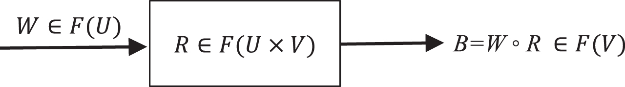
The FCE model.
To explain the FCE clearly, a simple example is shown here. For a given iris plant sample, after measuring, we have its Sepal Length = 5.2, Sepal Width = 3.7, Petal Length = 1.8, and Petal Width = 0.5. We know that there are three types of iris plants, Iris-setosa, Iris-versicolour, and Iris-virginica, and now, we need to decide which type this given sample belongs to. In this example, four influence factors constitute the factor set U = {Sepal Length, Sepal Width, Petal Length, Petal Width}, and three evaluation remarks constitute the decision set V = {Iris-setosa, Iris-versicolour, Iris-virginica}. We assume its fuzzy relational matrix and weight vector are respectively calculated to be (for the calculation methods, refer to the above presentation)
Then, according to the FCE model B = W ∘ R and the weighted average operator, we obtain
Due to 0.59 > 0.24 > 0.17, which implies the membership degree to Iris-setosa is the largest one, the evaluation result is Iris-setosa by the principle of maximum membership. That is, the given iris plant sample belongs to Iris-setosa.
Before introducing the proposed method, we give a basic presentation on classification:
The classification method [29] is a common data mining technique, and many classification methods have been proposed, such as support vector machine, decision tree, artificial neural network, and Naive Bayes rule. Classification has been extensively applied to image classification, document classification, sentiment analysis, spam mail filtering, disease prediction and so on [30]. Let D be a classification dataset with n distinct attributes a1, a2, ⋯ , a n . (we denote A = {a1, a2, ⋯ , a n }), |D| be its number of cases or transactions, and C ={ c1, c2, ⋯ , c m } be its list of class labels. Then, the i-th case in D can be described as a combination of attribute values d ij corresponding to the attribute a j and a class label c k (i = 1,2,⋯,|D|; j = 1,2,⋯,n; k = 1,2,⋯,m). In the classification process, D is first partitioned into two subsets, a training set (denoted as D train ) and a test set (denoted as D test ). The goal of classification is to build a classification model by D train , which can accurately predict a class lal from C for any case in D test . In addition, the model is evaluated by classification accuracy τ/|D test |. where τ is the number ocases that their predicted class labels are exactly their actual class labels, and |D test | is the number ocases in D test .
Now, let us compare the classification dataset D with the four components of the FCE. In other words, we wilsee the classification problem from the FCE viewpoint. We notice that the list of attributes A can be regarded as the factor set U, the list of class labels C can be garded as the decision set V, and the predicted class label can be regarded as the evaluation result in the FCE. Thus, the FCE model is actually a classifier, and thenly thing we need to do is to generate a reasonablfzy relational mrix R and a suitable weight vector W by D train , such that the FCE model B = W ∘ R can be carried out.
In this study, R is constructed by the joint distribution dynamic membership degree and W is constituted by equal weight, both of which will be introduced in Section 3.1 and Section 3.2, respectively. Therefore, our proposed classifier is called the fuzzy comprehensive evaluation based on the joint distribution dynamic membership degree (FCE-JDDMD).
The FCE-JDDMD classifier consists of six phases: input a classification dataset, data preprocessing (which refers to discretizing continuous attribute values), construct the fuzzy relational matrix R, input the weight vector W, implement the FCE model, and output a class label. The overall architecture of the FCE-JDDMD classifier is shown in Fig. 2.
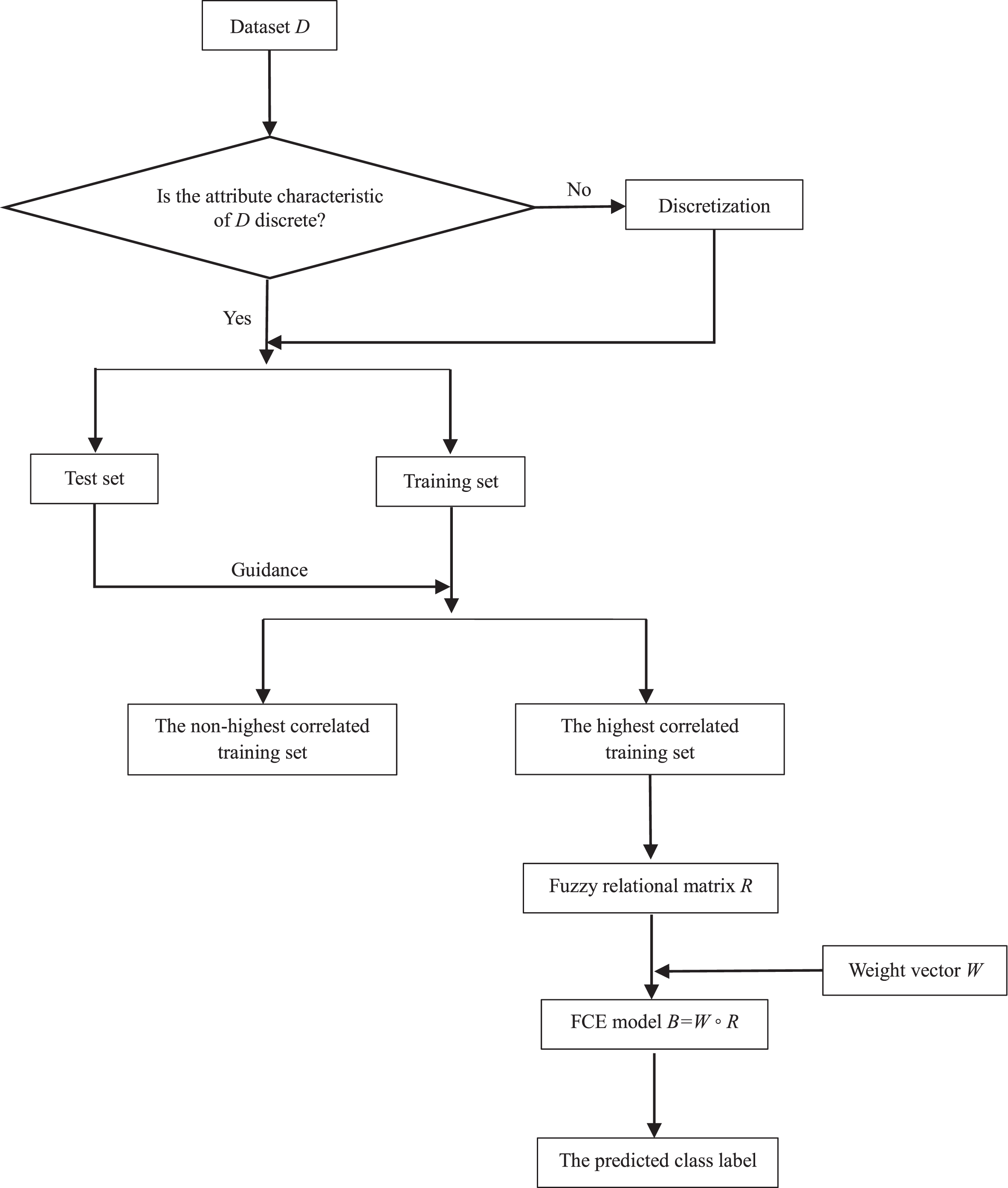
Overall architecture of the FCE-JDDMD classifier.
In this study, we divide datasets into three categories according to their attribute characteristics: discrete, continuous, and combined. An attribute is called a discrete attribute if its attribute values are nominal or categorical, and it is called a continuous attribute if its attribute values are real. If a dataset consists of discrete attributes, then it is called a discrete dataset, and if it is composed of continuous attributes, then it is called a continuous dataset. A combined dataset refers to a dataset that has both discrete attributes and continuous attributes.
In this section, for a discrete dataset, we propose the joint distribution dynamic membership degree (JDDMD) to construct R; for a continuous dataset or a combined dataset, we employ the equidistant discretization to convert it to a discrete dataset.
The construction of R in a discrete dataset
In this section, we will present the JDDMD in detail. The JDDMD is an improvement method of the static membership degree (SMD) which is also proposed by this study, so we will present the SMD first.
(1) SMD
Let D be a classification dataset with n distinct attributes a1, a2, ⋯ , a n , |D| be its number of cases, and C ={ c1, c2, ⋯ , c m } be its list of class labels. In a discrete dataset, for a given attribute a j 0 (j0∈{1,2,⋯,n}), its distinct attribute values are limited and we denote them as e1, e2, ⋯ , and e l . Furthermore, for a given h0∈{1,2,⋯,l}, we assume the number of e h 0 is s in D. Apparently, there is a list of class labels corresponding to e h 0 , and we denote it as C′. Meanwhile, we let c k 0 ∈ C′ (k0∈{1,2,⋯,m}) and assume the number of c k 0 is t in these s cases. Now, it can be seen as a scene like this: there are s persons to decide a class label from C for the attribute value e h 0 and t persons choose the class c k 0 , which exactly conforms to the idea of the fuzzy statistic method. Thus, t / s is the membership degree of attribute value e h 0 to class c k 0 .
In particular, when s = 0, it implies there is no person to decide a class label for e h 0 ; and in this study, we define: if s = 0, then the membership degree is 0.
The mathematical description of the SMD is as follows.
In the dataset D, for the i-th case, we let d
ij
be its attribute value corresponding to the attribute a
j
and c (i) be its class label. Then, for a given case
where j = 1,2,⋯,n; k = 1,2,⋯,m;
To clearly explain the construction of R using the SMD, a simple example is shown here.
A discrete classification dataset
*TID: transaction id.
We consider the given case d′=(3,2,3,3). a) For the attribute a1, there are five cases whose attribute values are 3: TID = 14, TID = 15, TID = 16, TID = 17, and TID = 18 (i.e., s = 5). In these five cases, the numbers of class 1 and class 2 are 3 and 2, respectively (i.e., t = 3 and t = 2, respectively). Therefore, the membership degrees to class 1 and class 2 are
(2) JDDMD
In practice, we noticed that the SMD might lead to an unreasonable evaluation vector. The following is a simple example.
Assume we have a dataset such as that shown in Table 3. Now, let us construct the fuzzy relational matrix R for the given case d′= (1,1).
A discrete classification dataset
*TID: transaction id.
According to Equation (1), we obtain
We assume that W = (w1, w2) is the corresponding weight vector, where w1 + w2 = 1. Then, regardless of the value of W, when we use the weighted average operator (i.e.,
This evaluation vector implies that the membership degree of the given case d′ to class 1 is 0.5 and to class 2 is also 0.5. Because the given case is the same as the first case in Table 3, we believe that they should have the same class label; that is, the given case should definitely belong to class 1, which means the evaluation vector should be (1,0). Thus, the above evaluation vector B = (0.5,0.5) is suspicious. Since B = (0.5,0.5) is unrelated to W, the problem must lie in the SMD. Hence, we come up with the dynamic membership degree, which is based on the joint distribution of attribute values. Its mathematical description is as follows.
Let D be a classification dataset with n distinct attributes a1, a2, ⋯ , a
n
, |D| be its number of cases, C = {c1, c2, …, c
m
} be its list of class labels, and d
ij
be the attribute value of the i-th case corresponding to the attribute a
j
(i = 1,2,⋯,|D|.; j = 1,2,⋯,n). For a given case
Now, considering Table 3, let us construct R for the given case d′= (1,1) using the JDDMD. First, the JDCNs of the given case to each case in Table 3 are calculated by Equation (2), and they are shown in Table 4.
Table 3 with the JDCN
* TID: transaction id.
So, the highest JDCN θ=max{2,0,1} = 2. Then, we have T = {1}. Hence, the highest correlated dataset D′ is (seen in Table 5)
The highest correlated dataset
* TID: transaction id.
Finally, according to D′, d′= (1,1) and Equation (1), we get the fuzzy relational matrix
Furthermore, let us check the evaluation vector after using the JDDMD:
Next, let us discuss the difference between the SMD and the JDDMD. It is not difficult to find that the former is calculated based on the original dataset D and the latter is calculated based on the highest correlated dataset D′ which is a subset of D. Let
First, the JDCNs are calculated by Equation (2), and they are shown in Table 6.
Table 2 with the JDCN
* TID: transaction id.
So, the highest JDCN θ=max{0,1,2,3} = 3. Then, we have T = {12,17,18}. Therefore, the highest correlated dataset D′ is (seen in Table 7)
The highest correlated dataset
* TID: transaction id.
Then, according to D′, d′= (3,2,3,3) and Equation (1), we obtain the fuzzy relational matrix
For a continuous dataset, we use discretization techniques to convert it to a discrete dataset, and then R can be constructed by the method in Section 3.1.1. It should be noted that each continuous attribute needs to be discretized, and in this study, we let they have the same discretization class number.
In this study, the equidistant partition, which divides continuous values into several finite intervals and each interval has the same length, is adopted to discretize. Thus, our discretization process can be described as follows.
We assume that a
j
0
is a continuous attribute and d
ij
0
is its attribute value (i = 1,2,⋯,|D|). Let
Next, let us discuss the determination of the discretization class number k. Since this research is devoted to the classification problem, apparently we can experiment with several values of k and then select the one with the highest classification accuracy as the optimal discretization class number. In this paper, we experiment k = 2, 3, 4, 5, 6, 7, 8, 9, and10. Hence, the optimal discretization class number
Because
A continuous classification dataset
* TID: transaction id.
For the attribute a1, we have
For the attribute a2, we have
The final discretization result is shown in Table 9.
The discretization result of Table 8
*TID: transaction id.
For the given case d′=(5.1,3.1), according to the above I1, I2 and I3, its discretization result is d′=(1,2). Then, its JDCNs can be calculated by Equation (2), and they are shown in Table 10.
Table 9 with the JDCN
*TID: transaction id.
Therefore, the highest JDCN θ=max{0,1,2} = 2. Then, we have T = {1,2}. So, the highest correlated dataset D′ is (seen in Table 11)
The highest correlated dataset
* TID: transaction id.
Finally, according to Equation (1), the fuzzy relational matrix is calculated to be
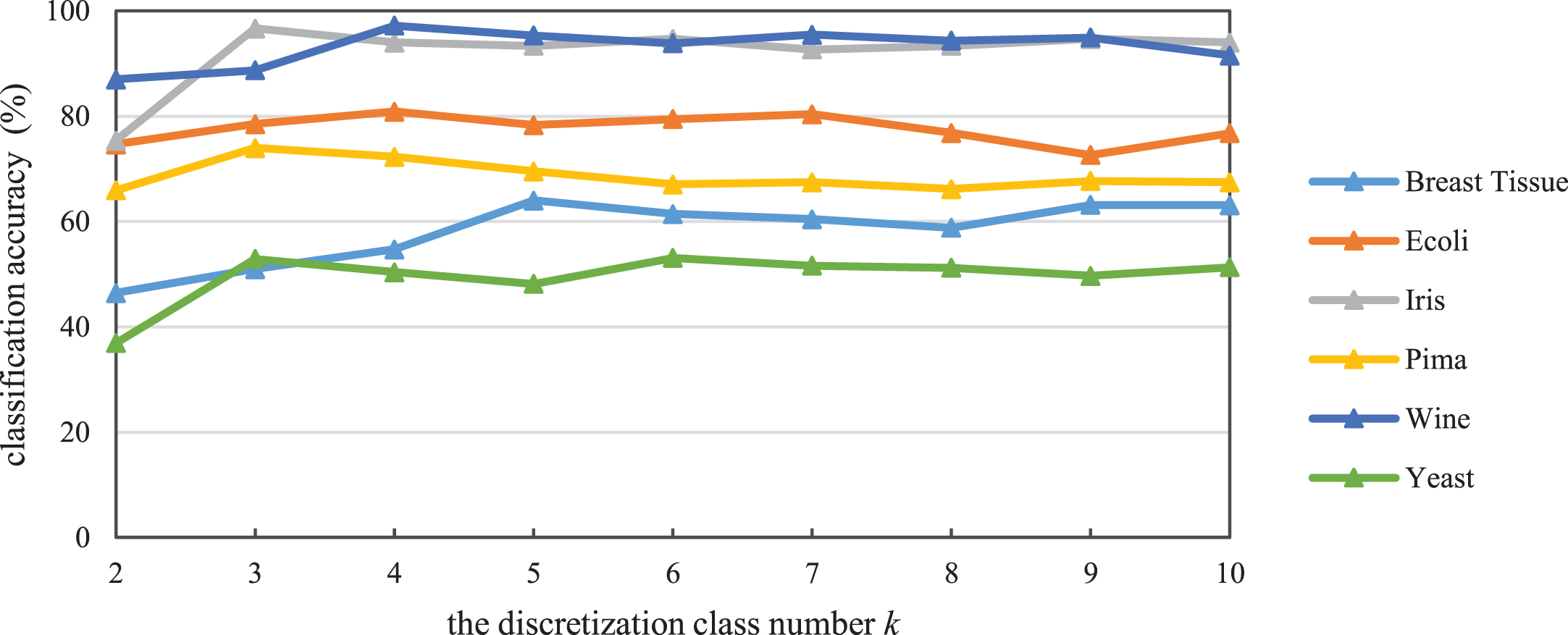
The influence of the discretization class number k on the proposed FCE-JDDMD classifier.
Following the approach used for the continuous dataset, we employ the equidistant discretization to convert a combined dataset to a discrete dataset. For details, please refer to Section 3.1.2.
The construction of W
Weight reflects the importance of an attribute. In this study, we choose equal weight to constitute the weight vector W. That is, W=(
Before deciding to use equal weight, we also attempt another two types of weight: optimization weight and entropy weight. However, we eventually found that they were all not appropriate. a) We form an optimization function that maximizes classification accuracy of the training set to calculate the optimization weight. However, the solution of this optimization function is generally not unique, and the solutions may lead to different classification results for a given test case, which is unacceptable in the classification problem. So we give up the optimization weight. b) When we consider using entropy as weight, dynamic entropy corresponding to the JDDMD arises, and this evidently will lead to more calculation. Since equal weight is simple and does not require additional calculation, we finally choose it as the weight of the attribute.
Model implementation
In a classification problem, the dataset is first divided into two subsets, a training set and a test set. For each case of the test set, according to Section 3.1 and Section 3.2, we can construct its fuzzy relational matrix R and weight vector W based on the training set. Then, the FCE model B = W ∘ R can be implemented, and the evaluation result (i.e., the predicted class label) is obtained. The steps of the proposed FCE-JDDMD are summarized in Algorithm 1.
For a test case, the time complexity of the FCE-JDDMD is O(|D|mn) where |D| is the number of cases in the dataset D, m is the number of class labels and n is the number of attributes. In addition, there are no parameters in the proposed classifier for a discrete dataset, and there is only one parameter for a continuous dataset or a combined dataset (i.e., the discretization class number). Thus, the proposed FCE-JDDMD classifier is simple.
Examples
In this section, we design two examples (a discrete classification problem and a continuous classification problem) to illustrate the proposed classifier. About the operator ∘ in the FCE model, this paper uses the weighted average operator, that is
Discrete training data and test data
Discrete training data and test data
* TID: transaction id.
Seeing Table 12 from the perspective of the FCE,
we have the factor set U = {a1, a2, a3, a4} and the decision set V = {1,2}.
For the test cases d′=(3,2,3,3) and d″=(2,1,1,2), according to the calculation of the JDDMD, their fuzzy relational matrices are respectively calculated to be
and
By the construction of W in Section 3.2, we obtain the weight vector is
W = (0.25,0.25,0.25,0.25).
Then, we input R′, R″, and W into the FCE model B = W ∘ R, and we get
As 0.67 > 0.33 and 1 > 0, the evaluation results are class 1 and class 2, respectively, according to the principle of maximum membership. That is, the predicted class label is class 1 for the test case TID = 19, and it is class 2 for TID = 20.
Continuous training data and test data
* TID: transaction id.
Observing Table 13 from the FCE point of view, we have the factor set U = {a1, a2} and the decision set V = {1,2}.
We assume the discretization class number is 3 (i.e., k = 3). Then, for the test cases d′=(5.1,3.1) and d″=(6,2.9), according to the equidistant discretization and the calculation of the JDDMD, their fuzzy relational matrices are respectively calculated to be (seen in Example 3)
According to the construction of W in Section 3.2, the weight vector becomes
W = (0.5,0.5).
By inputting R′, R″, and W into the FCE model, we obtain
Thus, when k = 3, the predicted class labels are all class 1. So, CA(3) = 50%.
The same to k = 2, 4, 5, 6, 7, 8, 9, and 10, we finally get
CA(2) = CA(4) = CA(7) = CA(9) = 100%,
CA(5) = CA(6) = CA(8) = CA(10) = 50%.
According to Equation (5), we have the optimal discretization class number
In this section, we empirically evaluate our proposed classifier icomparison with some other classifiers.
Experimental setting
The experiments are set as follows.
Twelve UCI datasets used in the experiments
Twelve UCI datasets used in the experiments
*The number of attributes does not include the sequence name of the dataset.
The experimental results are presented in Table 15, where the boldface entries indicate the best values. In Table 15, XGBoost is from https://github.com/dmlc/xgboost, while AdaBoost and SVM are from the machine learning toolkit scikit-learn. The maximum numbers of estimators for both XGBoost and AdaBoost are set to 50. For SVM, the parameter C = 1.0 and the kernel function uses the RBF kernel. Other relevant parameters use the default settings of their interfaces. In addition, the classification accuracy of RIPPER, CBA, MCAR, PCAR, and PCAR2 is from reference [30].
Classification accuracy (%) and rank of the proposed classifier against others
Classification accuracy (%) and rank of the proposed classifier against others
*
The effectiveness of the proposed classifier is discussed in two aspects: average accuracy and average rank.
(1) Average accuracy
As shown in Table 15, the FCE-JDDMD has the highest accuracy on 2 datasets (Monks1 and Iris) and has relatively high accuracy on 6 datasets where its rank is 2 or 4 (Balance, Breast-w, Monks2, Breast Tissue, Ecoli, and Wine). In particular, although the FCE-JDDMD ranks 5 on Tic-tac-toe, it actually has the second highest accuracy. In addition, the accuracy is compact on Monks3; although the accuracy of our classifier is relatively low, the accuracy gap between our classifier and the best classifier is only 98.74–97.47% = 1.27%. Overall, the average accuracy of the FCE-JDDMD is 85.20 which is the second highest, and it is lower than that of XGBoost and higher than that of the other classifiers. Therefore, the proposed classifier outperforms some existing classifiers in terms of classification accuracy.
In addition, although the average accuracy of the FCE-JDDMD is lower than that of XGBoost, since the FCE-JDDMD has at most one parameter as stated in Section 3.3, it is simpler than XGBoost.
(2) Average rank
To conduct a fair comparison, the Friedman test for average ranks is performed [31, 34]. This test is a non-parametric equivalent of the repeated-measures ANOVA (analysis of variance) and was proposed by Milton Friedman in 1937 [35, 36].
During the Friedman test, we first need to rank the classifiers for each dataset. That is, the best performing classifier obtains the rank of 1, the second best obtains the rank of 2, and so on. Particularly, when two classifiers have the same performance, mean rank is assigned. We denote π
ij
as the rank of the j-th of M classifiers on the i-th of N datasets. Under the null-hypothesis, which states that all the classifiers are equivalent (that is, their average ranks
From the average ranks in Table 15, we can see that the FCE-JDDMD, XGBoost, SVM and PCAR rank fourth (with ranks 4.21, 4.00, 3.83 and 4.25, respectively), MCAR and PCAR2 rank fifth (with ranks 4.88 and 4.75, respectively), RIPPER and CBA rank sixth (with ranks 5.96 and 5.58, respectively), and AdaBoost ranks eighth (with rank 7.54). That is, the FCE-JDDMD, XGBoost, SVM and PCAR are superior to the other classifiers. Next, we will test whether this conclusion is credible.
According to Equations (6) and (7), we have
With 9 classifiers and 12 datasets, F F is distributed according to the F-distribution with 9–1 = 8 and (9–1)×(12–1) = 88 degrees of freedom. Upon consultation, we know that the critical value of F(8,88) is 1.74 for α = 0.1. Due to F F > F0.1 (8, 88) (8,88), we reject the null-hypothesis. This means that these 9 classifiers are not equivalent and the above conclusion is credible. That is, the proposed FCE-JDDMD, XGBoost, SVM and PCAR indeed perform better than the other classifiers.
In conclusion, the proposed FCE-JDDMD has the second highest average accuracy and a headmost average rank. Thus, it is an outperforming classifier.
This paper puts forward a new classification method based on the FCE. The underlying idea is to regard the class labels in classification problems as the evaluation remarks in the FCE and regard their attributes to be consistent. So, the classification principle of the proposed FCE-JDDMD classifier is to provide the most probable class label to the object by comprehensively considering the membership degrees of every attribute to class labels. In the proposed classifier, for a discrete classification dataset, the JDDMD is put forward to construct the fuzzy relational matrix and equal weight is considered to constitute the weight vector, then the FCE model is executed to obtain the classification result; for a continuous classification dataset, the equidistant discretization is employed to convert it to a discrete dataset, and the determination of the discretization class number is also discussed in this study. Finally, we empirically demonstrate, on a variety of datasets, that the proposed classifier outperforms some existing classifiers.
The proposed FCE-JDDMD classifier not only has good interpretability but is also easy to operate. Therefore, from the perspective of the FCE, this study extensively extends the application of the FCE, such that the FCE innovatively advances in data mining; from the classification viewpoint, this study proposes a novel, simple and outperforming classification method.
Despite the aforementioned advantages, the proposed FCE-JDDMD has several limitations. For one thing, this study adopts equal weight as the attribute weights, which is subjective weight. In future work, we will attempt to design a learning algorithm to calculate the weight to improve the FCE-JDDMD. For another, in this study, we let each attribute have the same discretization class number for a given continuous dataset, and the work that assigning different discretization class numbers to attributes is a worthwhile future research.