Sage Journals: Discover world-class research

Abstract

Since it satisfies all prerequisites for the growth of humanity, agriculture is currently regarded as being the most significant sector for civilization. One of the main forms of human energy production is thought to be plants, which also provide nutrients, cures, etc. Any damage or disease brought on by exposure to pathogens, viruses, bacteria, etc., while cultivating plants results in a decline in productivity, making it crucial to prevent such diseases and take the required precautions to avoid them. Accurately identifying such fatal diseases is a crucial first step for both the businesses and farmers. Six different Convolutional Neural Networks (CNNs) that accept plant leaf images as input, along with the Enhanced Symbiotic Organism Search (ESOS) optimization algorithm, have been implemented in our research. We intend to extensively contrast the various models based on accuracy, precision, recall, and F1-score. In the area of image recognition and classification, convolutional neural networks (CNNs), in particular, and deep learning, in general, are developing. The literature contains a variety of CNN designs. The dataset size, the number of classes, the model’s weights, hypermeters, and optimizers are a few examples of the variables that have an impact on a CNN model’s performance. Because of its benefits, transfer learning and fine-tuning a pre-trained model are now very popular. This study examines the impact of six popular CNN models: DenseNet, MobileNet, EfficientNet, VGG19, ResNet and Inception. As a result, DenseNet demonstrates an optimal accuracy rate of 98% when compared to other models.

Keywords

Plant disease detection tomato plant leaf disease detection deep learning CNN DenseNet MobileNet EfficientNet VGG19 ResNet and inception

1 Introduction

India’s economy has grown significantly as a result of agriculture. Based on the soil type, weather in the area, and the crop’s economic value, the farmer chooses the necessary crop. Due to climate change and political uncertainty, the agricultural sector began looking for novel ways to increase food production because of population growth. This makes it possible for researchers to hunt for new, highly productive inventions that are precise and accurate. To decide how to maximize agricultural output, farmers can collect data and information using precise agriculture technologies. The economy of India and its population both significantly rely on agriculture. Typical leaf growth and color are two common indications that units suffered from distortion, development difficulties, withering, and damage. Although parasites and viruses can severely damage crops and spread disease to plants, they are also critically harmful to human health. The yields require meticulous inspection and appropriate management in order to guard against significant losses [2]. Plant infections can impact the leaves, stem, and natural products, among other parts of the plant. Over flowers and other natural objects, leaves provide some noteworthy points during all four seasons of the earth.

Climate change has considerably increased the likelihood of plant illnesses developing in the present. Plant diseases have a significant effect on their development, production, and quality. As a result, a technique for plant disease diagnosis and control at an early stage is needed. An early disease forecasting system must take into account crop phenology, meteorological factors, and the time of a disease’s attack. The date of the pest observation (BioFix) and the most recent meteorological data for a field are used to estimate pest assaults under field conditions. The forecast system’s main goals are to minimize the use of control methods and fungicides, as well as to minimize crop loss. To create a forecasting model, it is necessary to simultaneously monitor field micrometeorological parameters and pest/disease data. Identification and classification of plant diseases are based on the pathogens’ symptoms and indications. Numerous times, the detection of diseases on the basis of symptoms becomes extremely challenging. As a result, identification via digital images has been advancing. However, multispectral and hyperspectral photos are more expensive for farmers and offer less information.

2 Literature survey

Compared the capabilities of deep learning models, DenseNet, MobileNet, EfficientNet VGG19, ResNet, and Inception, to detect tomato plant diseases. The accuracy of disease classification obtained through experimentation and disease detection using deep learning approaches is pretty good. Table 1 illustrates the study of various deep learning models with their pros and cons.

Table 1
Literature review of various approaches with their pros and cons

Authors Pros Cons

R. Sujatha, Jyotir Moy Chatterjee, et al. (2021) [1] With layers and optimizers that assist in the development of a reliable model with increased accuracy. DL results are notable when compared to ML. Numerous metrics are taken into account, including area under the curve, F1 score, precision, and accuracy. Using a simple dataset improved classification accuracy, whereas using a large dataset could reduce classification accuracy.

S. Jain and D. Ramesh (2021) [2] Employed a Support Vector Machine (SVM) as a classifier and a deep convolutional neural network (CNN) as a feature extractor. The sole information offered by the SVM classifier with polynomial kernel function is classification accuracy and an F1 score.

Abbas, Amreen, Sweta Jain, et al. (2021) [3] The proposed approach successfully classified tomato leaf images into categories 5, 7, and 10 with an accuracy of up to 99.51%, 98.65%, and 97.11%, respectively. It has been demonstrated that this methodology beats the ones in use today. Overfitting is avoided by the C-GAN, which also improves network generalization. Although the detection of tomato disease was done on the leaves, the stems and branches of the plant must also be heavily engaged. The research was limited to the illness of tomato plants.

Sun, Henan, Haowei Xu, et al. (2021) [4] The outcomes demonstrated that the MEAN-SSD model, which attained 83.12 mAP and a pace of 12.53 FPS, is capable of identifying apple diseases with accuracy. The MEAN block is an essential component to speed up identification and reduce model size. Only five disease spots— Brown spot, Grey spot, Mosaic, Alternaria blotch, and Rust— were focused on in order to diagnose apple leaf diseases.

Hamdani, Anindita Septiarini, et al. (2021) [5] As seen by the high specificity, sensitivity, and accuracy values, which are near to 100%, 99.3%, and 99.67%, respectively, the classification results have demonstrated that the recommended method operates satisfactorily. Fewer features with stronger and more specialized attributes are produced by the methodology used. The classification outcomes demonstrate that an error was made because a leaf was incorrectly classified as healthy. The study’s sole focus was the oil palm leaf illness.

Pothen, Minu Eliz, et al., Pai (2020) [6] A polynomial kernel function and SVM Plus HOG can be used to identify additional plant diseases. The suggested research is pertinent and offers superior precision in comparison to other research. The LBP fundamental operator’s inability to record specific predominant traits is one of its drawbacks.

Mugithe, Pradeep Kumar, et al. (2020) [7] The disease’s effects In the graphical interface, Alternaria Alternata attained a precision of 95.16313%. The application of a disease detection warning device. Even the reported findings are not clear because the authors did not address any other diseases.

Nawaz, Muhammad Amir, et al. (2020) [8] The suggested IoT-based approach is inexpensive. Low-income farmers can buy it and use it to stop the spread of disease. The three factors of temperature, moisture, and leaf shade were the only ones the writers allowed in their model. The evaluated features for the criteria under consideration are inaccurate, which is another restriction. Additionally, a variety of features that could change unexpectedly based on the surroundings were extracted from these parameters. The disease kinds are still unknown because the leaves of afflicted plants cannot be identified.

Mojjada, Ramesh Kumar, et al. (2020) [9] Using five classes of damaged leaf images found for corn, tomatoes, bell peppers, peaches, and grapes, the system was evaluated with a 75% accuracy rate. The article used many standard techniques.

Reddy, K. Ashish, et al. (2020) [10] This paper establishes a framework for the quick and precise identification of damaged images. When compared to other techniques, k-means clustering has higher accuracy and processes data faster. In this paper, very conventional and outdated methods were taken into account.

Authors	Pros	Cons
R. Sujatha, Jyotir Moy Chatterjee, et al. (2021) [1]	With layers and optimizers that assist in the development of a reliable model with increased accuracy. DL results are notable when compared to ML. Numerous metrics are taken into account, including area under the curve, F1 score, precision, and accuracy.	Using a simple dataset improved classification accuracy, whereas using a large dataset could reduce classification accuracy.
S. Jain and D. Ramesh (2021) [2]	Employed a Support Vector Machine (SVM) as a classifier and a deep convolutional neural network (CNN) as a feature extractor.	The sole information offered by the SVM classifier with polynomial kernel function is classification accuracy and an F1 score.
Abbas, Amreen, Sweta Jain, et al. (2021) [3]	The proposed approach successfully classified tomato leaf images into categories 5, 7, and 10 with an accuracy of up to 99.51%, 98.65%, and 97.11%, respectively. It has been demonstrated that this methodology beats the ones in use today. Overfitting is avoided by the C-GAN, which also improves network generalization.	Although the detection of tomato disease was done on the leaves, the stems and branches of the plant must also be heavily engaged. The research was limited to the illness of tomato plants.
Sun, Henan, Haowei Xu, et al. (2021) [4]	The outcomes demonstrated that the MEAN-SSD model, which attained 83.12 mAP and a pace of 12.53 FPS, is capable of identifying apple diseases with accuracy. The MEAN block is an essential component to speed up identification and reduce model size.	Only five disease spots— Brown spot, Grey spot, Mosaic, Alternaria blotch, and Rust— were focused on in order to diagnose apple leaf diseases.
Hamdani, Anindita Septiarini, et al. (2021) [5]	As seen by the high specificity, sensitivity, and accuracy values, which are near to 100%, 99.3%, and 99.67%, respectively, the classification results have demonstrated that the recommended method operates satisfactorily. Fewer features with stronger and more specialized attributes are produced by the methodology used.	The classification outcomes demonstrate that an error was made because a leaf was incorrectly classified as healthy. The study’s sole focus was the oil palm leaf illness.
Pothen, Minu Eliz, et al., Pai (2020) [6]	A polynomial kernel function and SVM Plus HOG can be used to identify additional plant diseases. The suggested research is pertinent and offers superior precision in comparison to other research.	The LBP fundamental operator’s inability to record specific predominant traits is one of its drawbacks.
Mugithe, Pradeep Kumar, et al. (2020) [7]	The disease’s effects In the graphical interface, Alternaria Alternata attained a precision of 95.16313%. The application of a disease detection warning device.	Even the reported findings are not clear because the authors did not address any other diseases.
Nawaz, Muhammad Amir, et al. (2020) [8]	The suggested IoT-based approach is inexpensive. Low-income farmers can buy it and use it to stop the spread of disease.	The three factors of temperature, moisture, and leaf shade were the only ones the writers allowed in their model. The evaluated features for the criteria under consideration are inaccurate, which is another restriction. Additionally, a variety of features that could change unexpectedly based on the surroundings were extracted from these parameters. The disease kinds are still unknown because the leaves of afflicted plants cannot be identified.
Mojjada, Ramesh Kumar, et al. (2020) [9]	Using five classes of damaged leaf images found for corn, tomatoes, bell peppers, peaches, and grapes, the system was evaluated with a 75% accuracy rate.	The article used many standard techniques.
Reddy, K. Ashish, et al. (2020) [10]	This paper establishes a framework for the quick and precise identification of damaged images. When compared to other techniques, k-means clustering has higher accuracy and processes data faster.	In this paper, very conventional and outdated methods were taken into account.

3 Dataset description

A publicly accessible dataset called PlantVillage was used to train all of the deep learning models. It includes 10,050 images of various healthy and diseased leaves associated with ten different classes (Fig. 1 displays several plant diseases). For the purpose of this article, the term “responsible party” refers to any person or organization that has the authority to act on behalf of another person or organization. The dataset was divided into three groups: training, validation, and testing datasets, correspondingly, to avoid overfitting.

Fig. 1

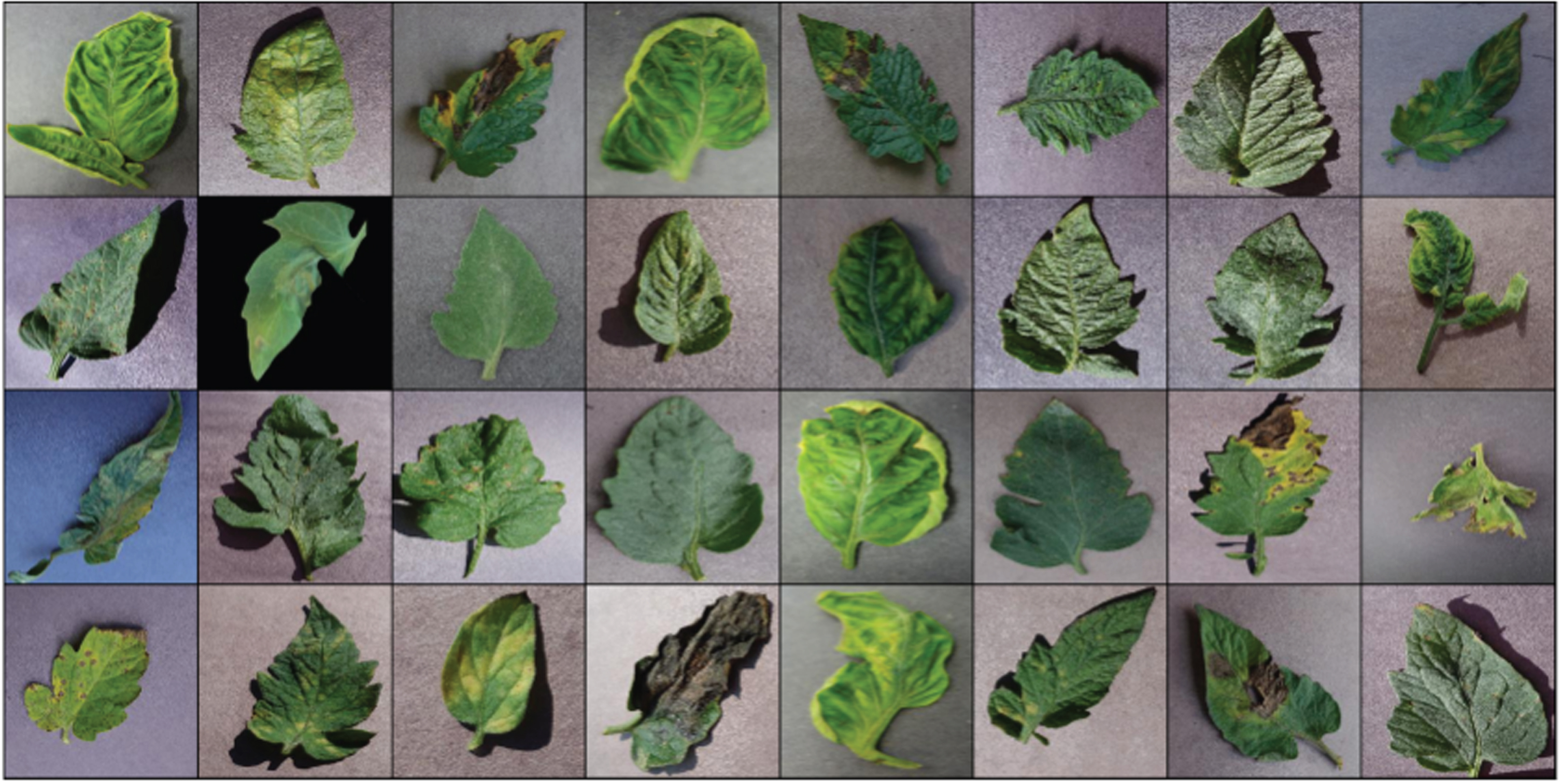
Sample images of diseased leaves.

4 ESOS algorithm

The symbiotic link between organisms in nature served as the inspiration for the metaheuristic optimization algorithm known as Enhanced Symbiotic Organism Search Optimization (ESOS). To resolve challenging optimization issues, it imitates the interactions and dynamics seen in ecological systems. Three different types of organisms— host organisms, symbionts, and free-living organisms— are used to mimic the optimization process in SOS. Each creature in the search space of the optimization problem indicates a potential solution.

The optimization process of SOS consists of the following steps:

Initialization: Produce a starting population of symbionts and hosts. Each organism should be given a fitness score based on an assessment of its function.

Symbiosis Phase: Engage in symbiotic relationships with symbionts and host organisms. They communicate and adjust based on their individual fitness levels. By collaborating with one another and exchanging knowledge, this stage seeks to improve the quality of solutions.

Reproduction Phase: From the symbiotic phase, pick the organisms that perform well. Reproduce, mutate, or recombine to produce new host organisms and symbionts.

Free-living Phase: Permit some creatures to exist separately from symbiotic relationships. Exploration of the search space is encouraged during this stage, broadening the range of potential solutions.

Evaluation of Fitness: Assess the level of fitness of the newly created organisms during the reproduction phase. Adapt the organisms’ fitness values based on the objective function.

Termination Criteria: Choose a condition for termination, such as reaching a particular solution quality or a set number of iterations.

The system seeks to discover optimal or nearly optimal solutions for the given optimization issue through the interactions and evolution of organisms in ESOS. It makes use of the cooperative, competitive, and adaptive processes found in natural ecosystems to effectively comb the search space and converge on promising answers.

4.1 Pseudocode for ESOS algorithm

START

Determine population size (n), objective function (X), limits on search variables (LB, UB), set count of searching variables (m), and g _ max (maximum generations) or set ending criteria (FE_max (maximum function evaluations) where f (X) denotes the objective function, and X indicates the search vector.

Initiating random population,

Compute the fitness of populations,

FE = 0,

FOR g = 1 to g _ max DO;

Sort the population in ascending order of f (x _ i) values,

Find the better solution (X_best) for the populations.

FORi = 1 to n Do

BF1 = 1 + round [rand (0,1)]

BF2 = 1 + round [rand (0,1)]

MV = (X_i + X_k)/2

FE = FE + 2

IF THEN

| X_{i} = X_{i}^{'}

END IF

IF THEN

| X_{k} = X_{k}^{'}

END IF

X_{i}^{'} = X_{i} + rand (- 1, 1) * (X_{best} - X_{k} k \neq 1

FE = FE + 1

IF f (X_i’) < f (X_i) THEN

| X_{i} = X_{i}^{'}

END IF

Choose Parasite Vector

FE = FE + 1

IF f (Parasite Vector) < f (X_k) THEN

|X_k= Parasite Vector

END IF

IF FE ≥ FE_max THEN

| Break optimization loop

END IF

END FOR

Report best solution

END

5 Deep learning architectures

The utilization of a deep learning architecture in conjunction with the ESOS algorithm presents a viable approach to augment the optimization procedure in the context of training. ESOS is an evolutionary optimization technique that draws inspiration from natural processes, specifically the principle of natural selection. Its purpose is to optimize the hyperparameters or parameters of a deep learning model.

5.1 DenseNet

Using Dense Blocks, which connect all layers (with matching feature map sizes) directly with one another, a DenseNet is a type of convolutional neural network that makes advantage of dense connections between layers [11]. Each layer receives new information from all layers that came before it and sends its own feature-maps to all layers that came after it in order to preserve the system’s feed-forward component. Each layer in the DenseNet transmits its own feature maps to all layers below it and gets new information from all levels above it [12]. Concatenation is employed. Each layer receives the “collective knowledge” of all layers underneath it. Figure 1a illustrates the basic block diagram of DenseNet architecture.

Fig. 1

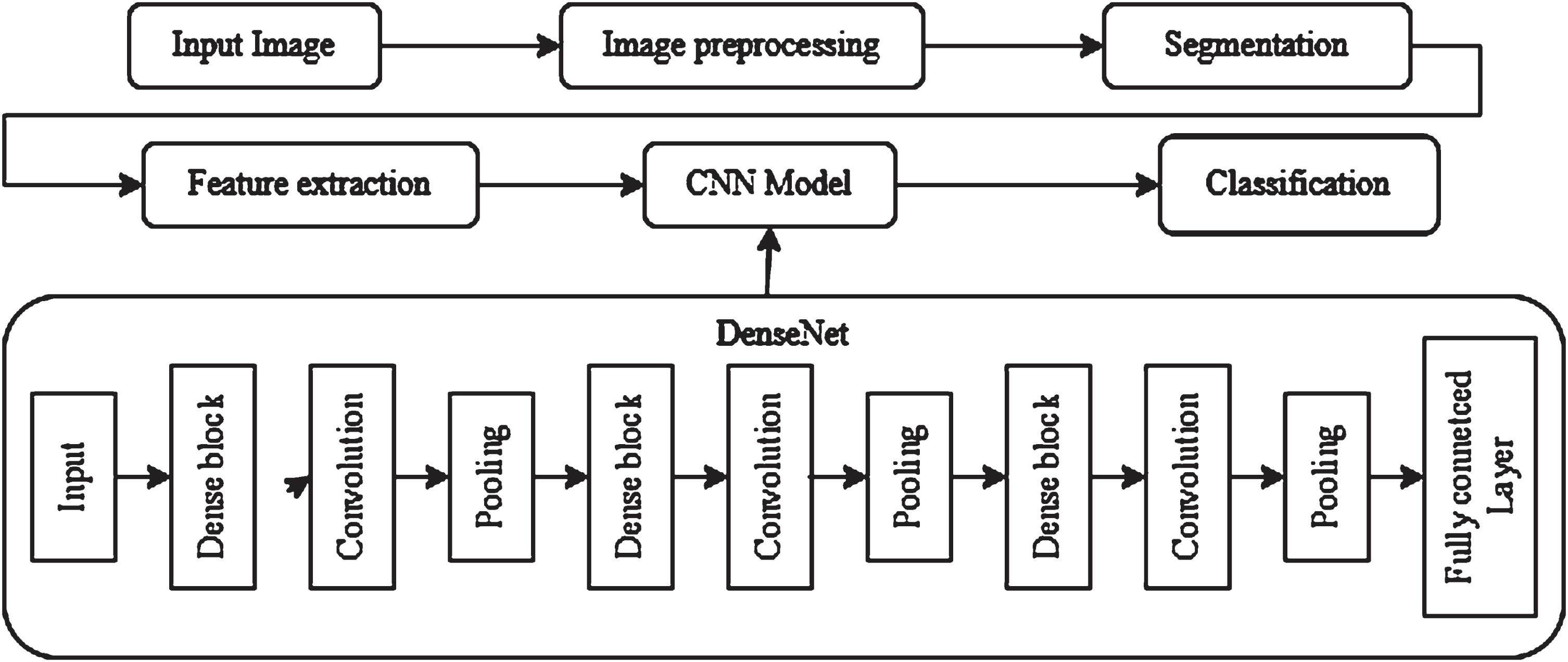
a). Block diagram of DenseNet architecture.

5.2 Inception

Extending GoogleNet is the 48-layered DCNN known as Inception. Convolution is a process that develops feature maps by using a combination of symmetric and asymmetric blocks implementing a filter to the picture input, computing the average from each patch’s feature map using standard pooling, Max-pooling, which optimizes the pixel and helps cut down on the amount of the parameters needed for learning [13], lowers processing costs. Concerts pool inputs of similar size and usually include dropouts after pooling, improving accuracy and reducing overfitting. Figure 1b illustrates the basic block diagram of Inception architecture.

Fig. 1

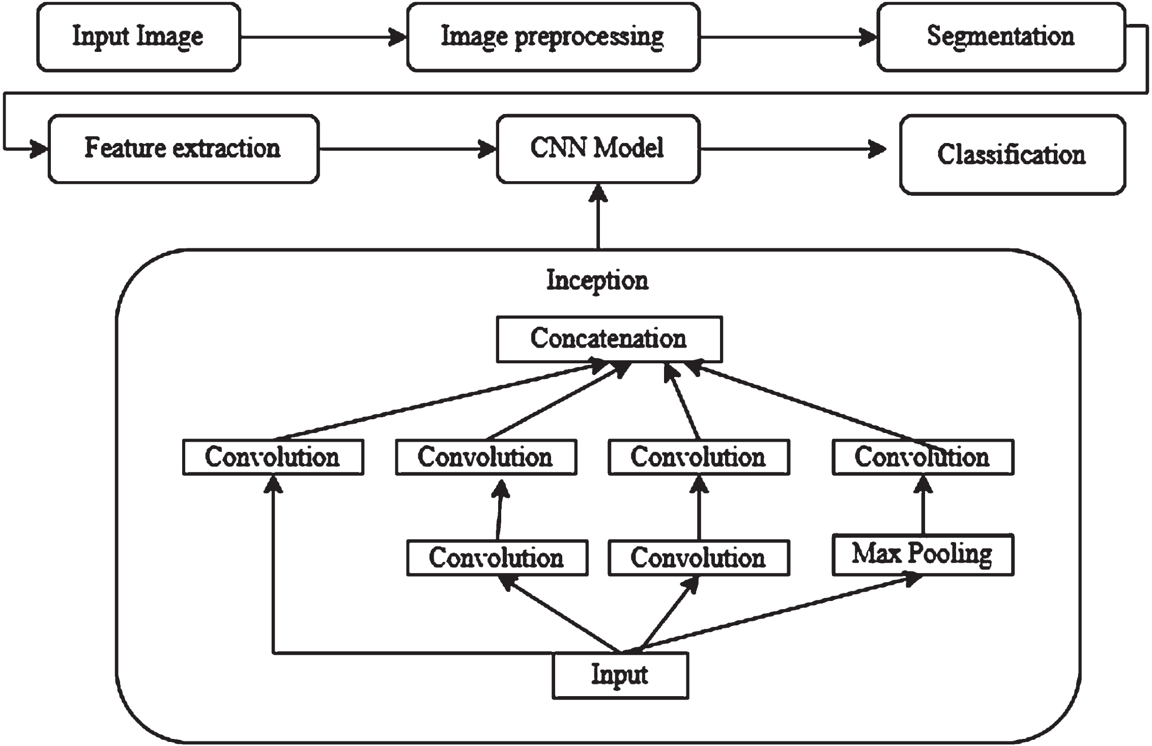
b). Block diagram of Inception architecture.

5.3 MobileNet

Google has made its open-source MobileNet machine vision model available for classification training. It creates a thin deep neural network by employing depthwise convolutions to dramatically lower the number of parameters compared to previous networks. The initial Tensorflow mobile computer vision model is known as MobileNet. When compared to other networks with normal convolutions and the same depth in the nets, depthwise separable convolutions dramatically reduce the number of parameters [14]. Lightweight deep neural networks are the outcome of this. Convolutional neural networks (CNNs) of the MobileNet class, which Google open-sourced, can be used to train extremely quick and compact classifiers. Figure 1c illustrates the basic block diagram of MobileNet architecture.

Fig. 1

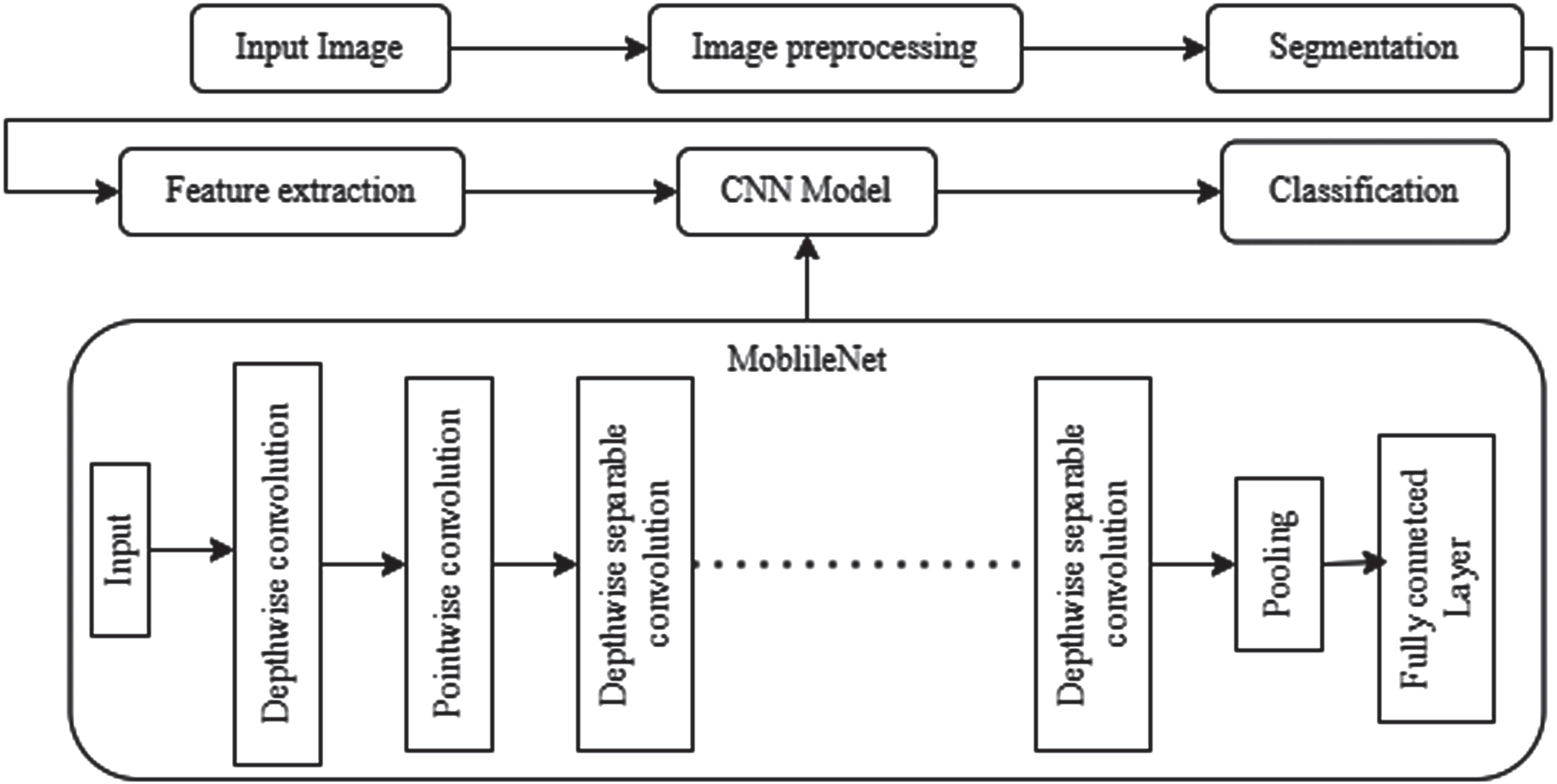
c). Block diagram of MobileNet architecture.

5.4 VGG19

Only the most powerful and predictive neurons are activated to produce a forecast after the network iterates through all of the training examples in forward and backward propagation. The training process for the model involves running all training samples twice, once forward and once backwards. When utilizing forward propagation, the loss and cost functions are calculated by comparing the anticipated target and the actual target for each tagged image [15]. Gradient descent is used through backward propagation to update each neuron’s weights and bias, providing greater weight to the neurons with the highest predictive potential until the best possible activation combination is found. Figure 1d illustrates the basic block diagram of VGG19 architecture.

Fig. 1

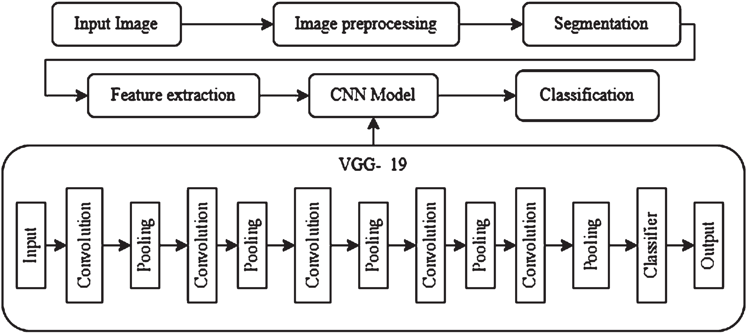
d). Block diagram of VGG19 architecture.

5.5 EfficientNet

The design tenets of EfficientNet centre on striking a balance between model correctness, computing effectiveness, and model complexity. It addresses the issue of creating models that are extremely accurate while also being computationally economical, which is essential for real-world applications where computational resources are frequently constrained. EfficientNet’s architecture is built on the idea of compound scaling, which entails uniformly increasing the network’s depth, width, and resolution. In comparison to earlier models that were individually optimized for depth or width, EfficientNet delivers improved performance by maintaining a balance between both scaling factors. The employment of a compound scaling formula by EfficientNet to establish the ideal scaling factors for depth, width, and resolution is one of its distinguishing characteristics [16]. This equation guarantees that the model obtains the best accuracy-to-efficiency ratio. EfficientNet improves accuracy while retaining processing economy by scaling up the network design. Figure 1e illustrates the basic block diagram of EfficicentNet architecture.

Fig. 1

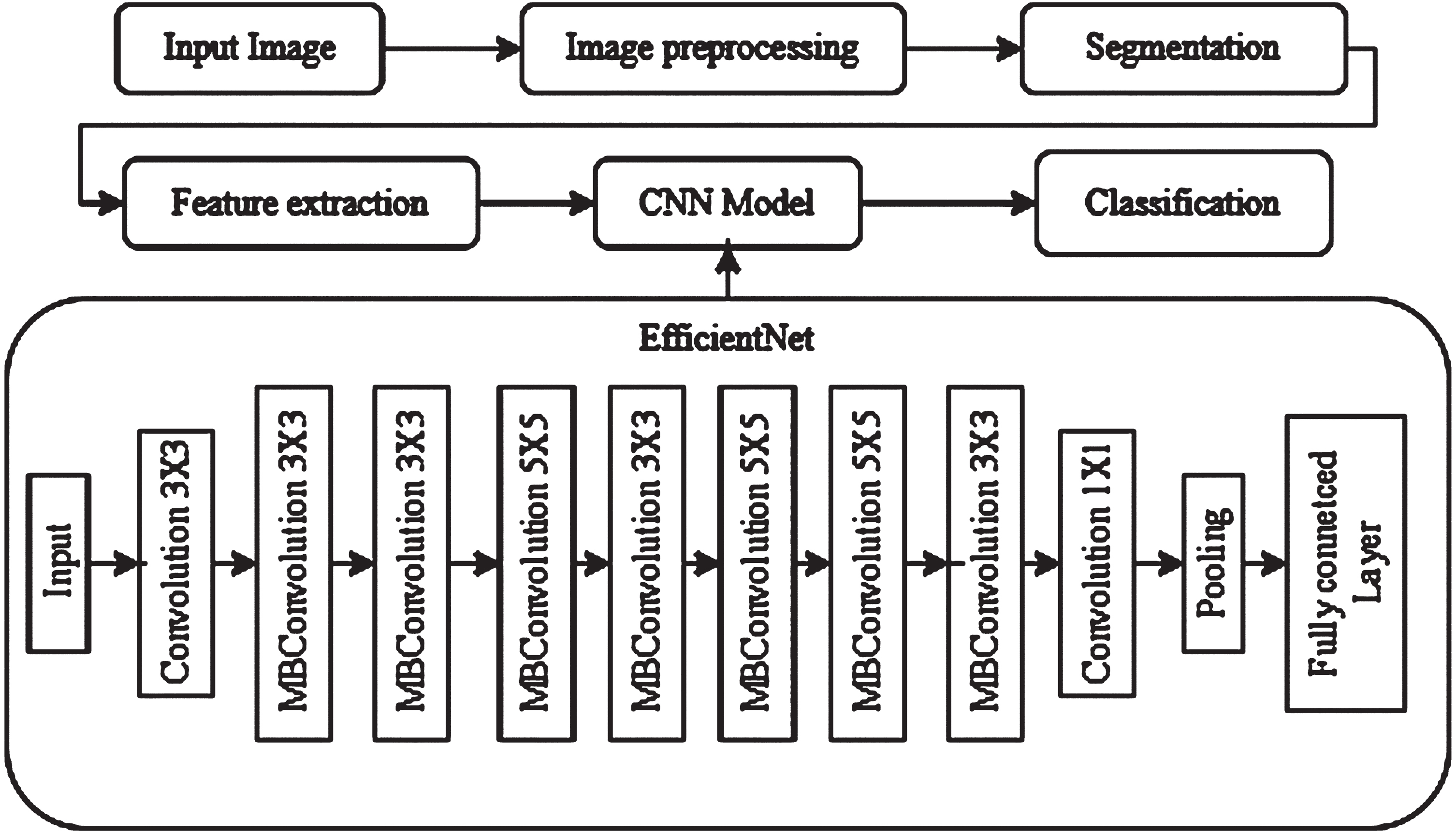
e). Block diagram of EfficicentNet architecture.

5.6 ResNet

ResNet’s ability to solve the issue of vanishing gradients in deep neural networks represents its main innovation. Gradients may become less pronounced as a network gets deeper, making it more difficult for it to learn and spread relevant information. The introduction of residual connections, also known as skip connections, which enable the network to skip some layers and immediately transfer data from previous layers to later ones, solves this issue. A residual block is the fundamental unit of a ResNet. A skip connection that adds the input to the block’s output comes after each residual block’s two or more convolutional layers [17]. ResNet topologies come in a variety of depths, with the number indicating the total number of layers in the network, such as ResNet-18, ResNet-34, ResNet-50, ResNet-101, and ResNet-152. On a variety of image classification tasks, deeper ResNet models have demonstrated enhanced performance, frequently outperforming shallower architectures. ResNet architectures have also been used for tasks including object detection, semantic segmentation, and picture synthesis, in addition to image classification [18]. ResNet is a popular option for researchers and practitioners in the field of computer vision due to its adaptability and efficacy. Figure 1f illustrates the basic block diagram of ResNet architecture.

Fig. 1

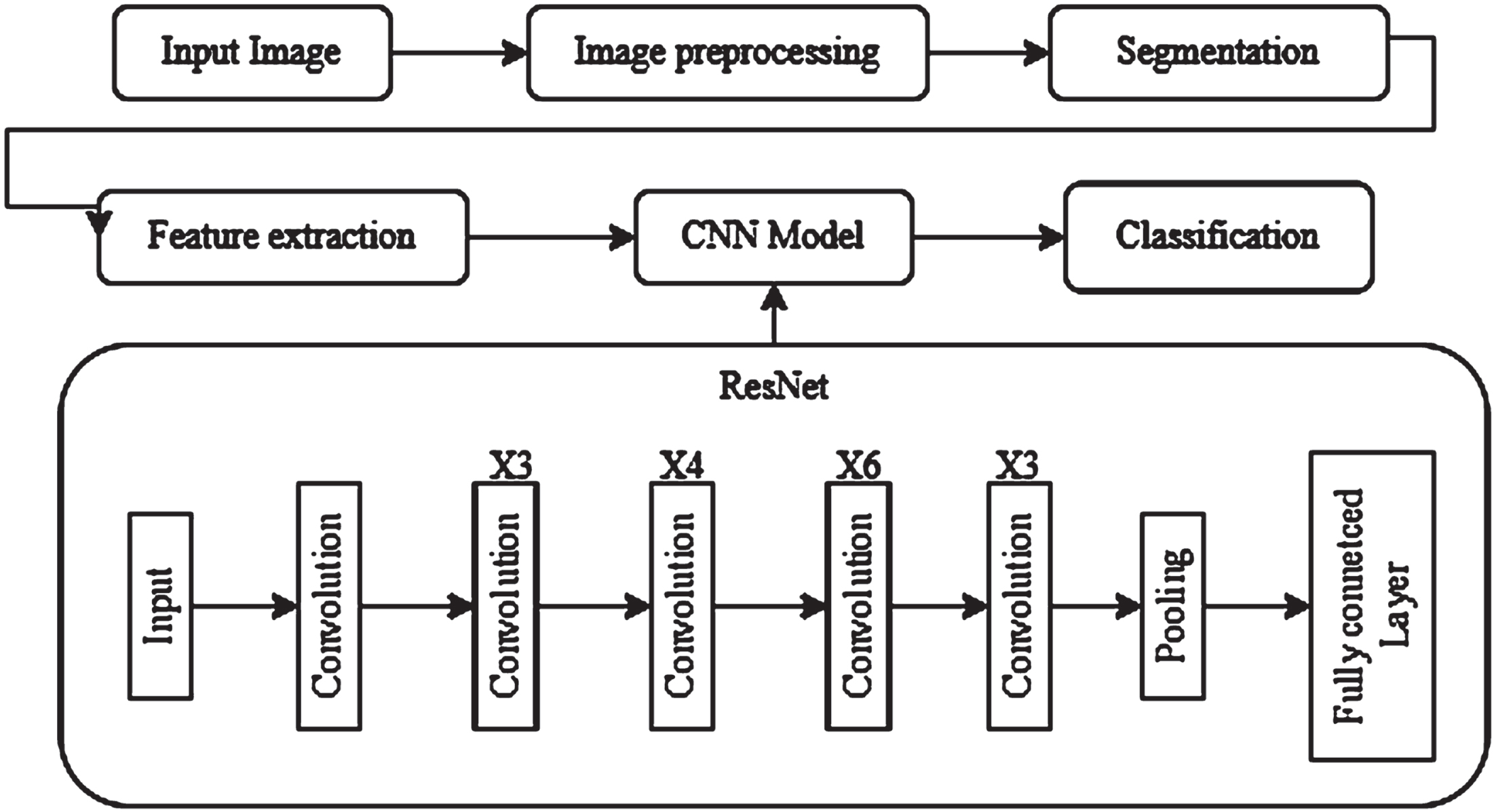
f). Block diagram of ResNet architecture.

6 Evaluation of performance metrics

In this section, we have evaluated each model using the accuracy, precision, recall, and F1-score result characteristics [19]. A comprehensive breakdown of each model’s output parameters can be found in Table 2.

Table 2
Exhaustive deterioration of model output parameters

Model Accuracy (%) Loss (%) Precision Recall F1-score

DenseNet 98 2 84 82 82

MobileNet 93 7 80 80 79

EfficientNet 95 18 78 77 76

VGG19 89 11 72 71 71

ResNet 95 5 76 75 74

Inception 96 4 74 73 72

Model	Accuracy (%)	Loss (%)	Precision	Recall	F1-score
DenseNet	98	2	84	82	82
MobileNet	93	7	80	80	79
EfficientNet	95	18	78	77	76
VGG19	89	11	72	71	71
ResNet	95	5	76	75	74
Inception	96	4	74	73	72

The highlighted values in Table. 2 above show the best model results. DenseNet did the best, producing 98% accuracy. Adam, a middling category optimizer, was used in this model’s configuration, and training took 156 seconds. The algorithms utilised had an accuracy of 89% and included MobileNet, EfficientNet, Resnet, Inception, and VGG19. Out of the six learnt models, the VGG19 model’s accuracy was the lowest. The Inception model took the longest (214 seconds), but it failed to get the desired results.

Accuracy is used to gauge performance; accuracy is calculated as the ratio of the model’s correct predictions to all other predictions. The average accuracy of the enhanced images with the various models is shown in Table 2. From Table 2, it can be found that the testing accuracies of DenseNet, MoibileNet, EfficientNet, VGG19, ResNet and Inception are 98%, 93%, 95%, 89%, 95% and 96%, respectively.

Furthermore, the performance’s recall, precision, and f1 score are assessed. Precision is defined as the ratio of the model’s true positive (TP) predictions to its total positive (TP+FP) projections. The subsequent standards are used to evaluate precision: $Precision = \frac{TP + FP}{TP}$

Figure 2 shows the precision of the various models. DenseNet yielded precision values of 84, MobileNet of 80, EfficientNet of 78, VGG19 of 72, ResNet of 76 and Inception of 74. The DenseNet model was observed to provide superior precision than other ensemble models. Recall is defined as the ratio of true positives (TP) to all sample data (TP+FN). Recall can be calculated using the formula below: $Recall = \frac{TP + FN}{TP}$

Fig. 2

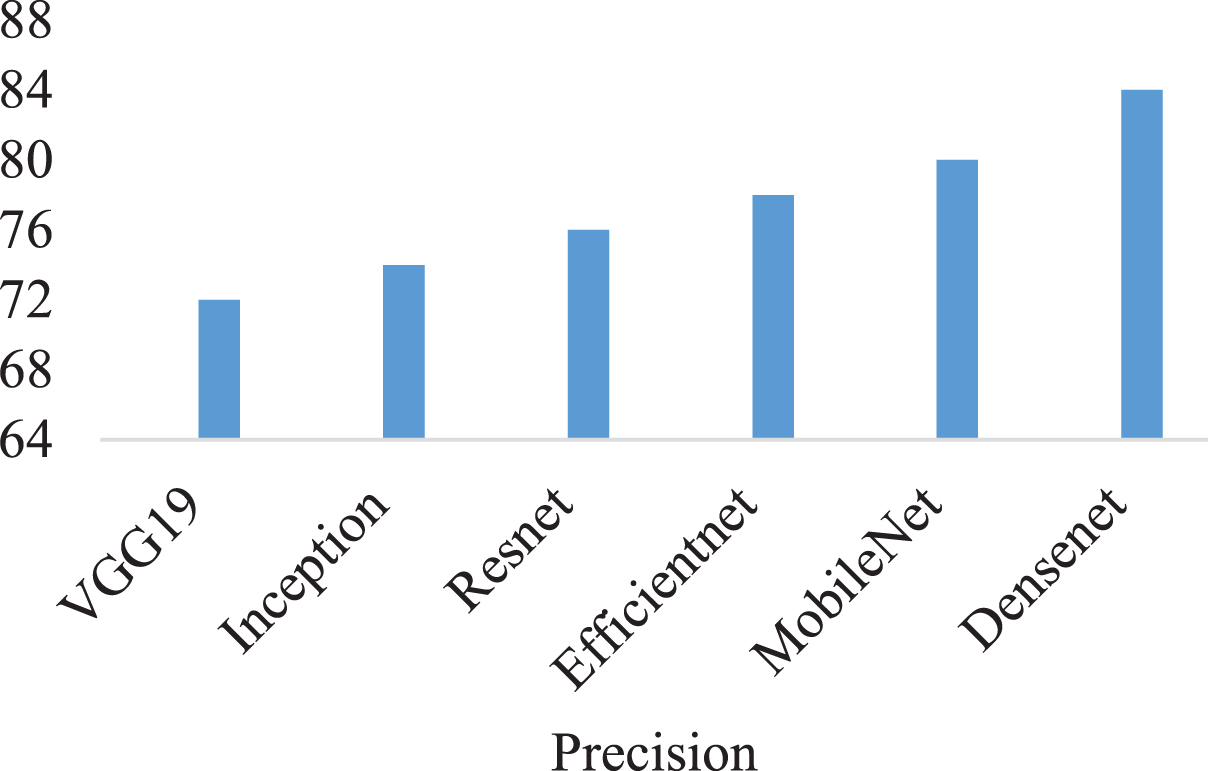
Comparing Precision Metrics across CNN Models.

The recall percentages for various models are shown in Fig. 3. Recall values DenseNet of 82, MobileNet of 80, EfficientNet of 77, VGG19 of 71, ResNet of 75 and Inception of 73. We can infer from the recall value that the DenseNet outperforms other deployed models. Another popular performance indicator for deep learning algorithms is the F1 score. The balance between recall and precision is expressed by the F1 score. The harmonic mean of recall and precision is used to calculate the F1 score. 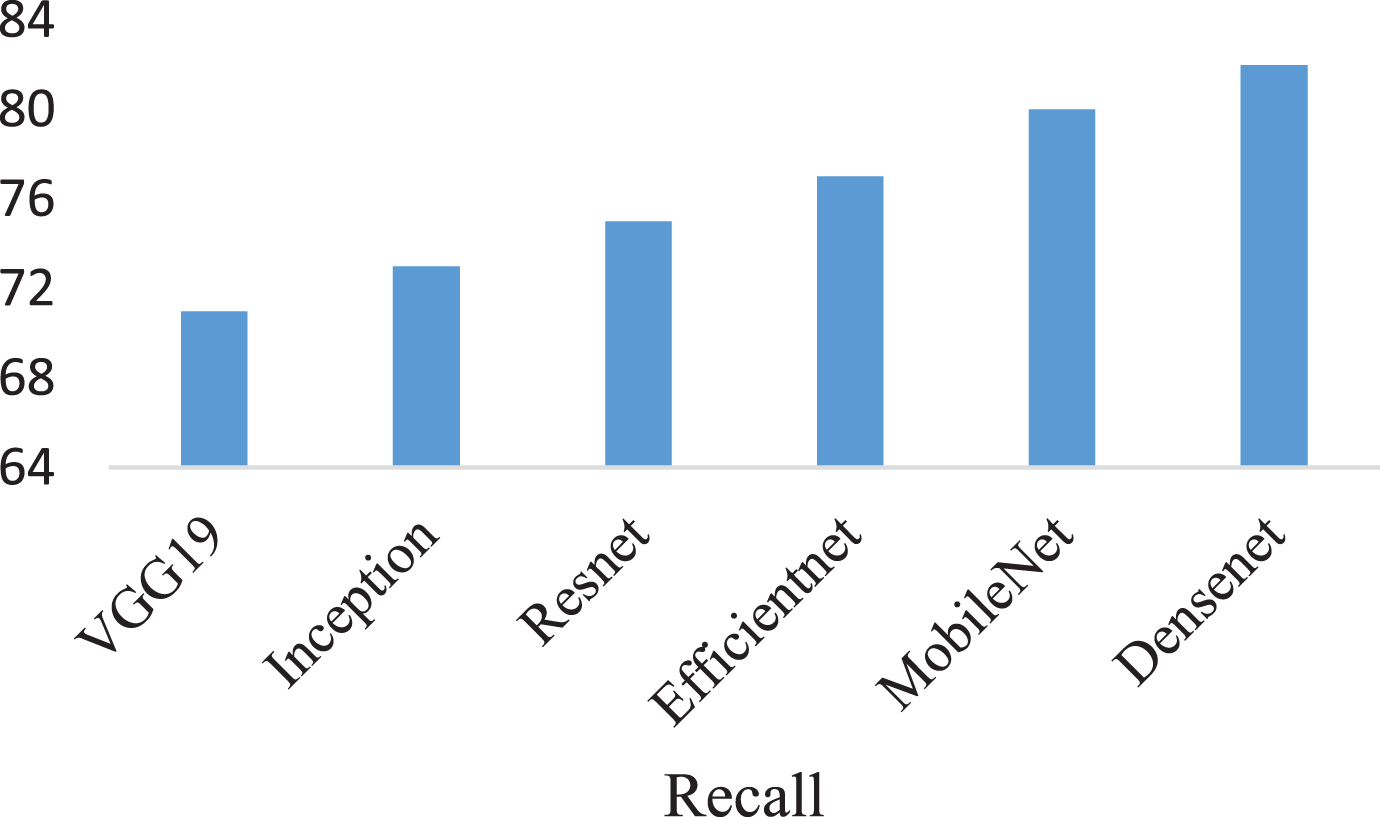The F1 score is determined by the following factors: $F_{1} score = 2 \times \frac{Precision \times Recall}{Precision + Recall}$

Fig. 3

Recall Evaluation across Different CNN Architectures.

The F1 scores for models are shown in Fig. 4. The F1 values that were attained were DenseNet of 82, MobileNet of 79, EfficientNet of 76, VGG19 of 71, ResNet of 74 and Inception of 72. We can infer from Fig. 4 that DenseNet perform better than other ensemble models.

Fig. 4

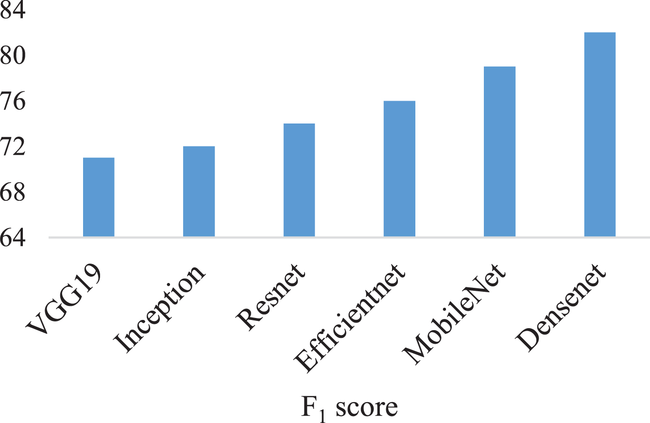
F₁ score Performance Assessment of CNN Models.

6.1 Comparison of existing deep learning algorithms for detecting plant diseases

In this section, using some of the existing deep learning models, such as DenseNet, MobileNet, EfficientNet, VGG19, ResNet, and Inception, we will assess the results of our proposed model. The number of parameters and classification accuracy of deep learning models are compared in Table 2. Additionally, when we compared the performance accuracy of our suggested CNN model with DenseNet to that of existing deep learning models, we discovered that it performed more accurately while using fewer parameters [20]. The accuracy of the suggested CNN with DenseNet is 98% with relatively few parameters, while MobileNet, EfficientNet, VGG19, ResNet and Inception are 93%, 95%, 89%, 95% and 96% accurate with more parameters, respectively.

Table 3
Comparison of six CNN models with and without ESOS algorithm

Model With ESOS algorithm Without ESOS algorithm

Accuracy Loss Precision Recall F1-score Accuracy Loss Precision Recall F1-score

DenseNet 98 2 84 82 82 87 7 74 76 76

MobileNet 93 7 80 80 79 82 12 72 74 73

EfficientNet 95 18 78 77 76 84 23 70 71 70

VGG19 89 11 72 71 71 78 16 66 65 65

ResNet 95 5 76 75 74 84 10 68 69 68

Inception 96 4 74 73 72 85 9 66 67 68

Model	With ESOS algorithm	Without ESOS algorithm
DenseNet	98	2	84	82	82	87	7	74	76	76
MobileNet	93	7	80	80	79	82	12	72	74	73
EfficientNet	95	18	78	77	76	84	23	70	71	70
VGG19	89	11	72	71	71	78	16	66	65	65
ResNet	95	5	76	75	74	84	10	68	69	68
Inception	96	4	74	73	72	85	9	66	67	68

7 Results and discussion

We examine how the ESOS algorithm affects CNN models for plant leaf disease detection. ESOS optimizes CNN model hyperparameters to increase performance. We train six CNN models, to evaluate the ESOS algorithm performance. Our investigations show that the models operate differently. ESOS-trained CNN models outperform those without hyperparameter optimization. ESOS-based models detect plant leaf diseases with greater accuracy, precision, recall, and F1-score. The ESOS approach increased CNN model performance, suggesting it might be used for hyperparameter optimization in deep learning-based plant disease detection applications. This study recommends integrating ESOS to maximize CNN model performance, develop precision agriculture, promote sustainable crop management. Comparison of six CNN models with and without ESOS algorithm integration is shown in Table 3.

The accuracy curves are presented in the following part in terms of epochs. Models such as DenseNet, MoibileNet, EfficientNet, VGG19, ResNet and Inception have been developed and imparted using the following criteria:

Metric: Accuracy and loss

No. of epochs: 15

Training & Validation: 10 batches

The Number of images in the entire Train dataset: 10050 for each class

Number of images overall in the validation dataset: 1050 for each class.

Figures 5 and 6, depict the training accuracy and loss curves, respectively, regarding the number of epochs for DenseNet, MoibileNet, EfficientNet, VGG19, ResNet and Inception. The Fig shows that while EfficientNet takes longer than other models to achieve the ideal value, it stabilizes after 5 or 7 epochs. According to Fig. 5, DenseNet has considerably greater accuracy than the other models for the provided dataset. DenseNet works better in terms of training accuracy than the other models. If there had been more than 15 epochs, DenseNet might have exhibited greater precision.

Fig. 5

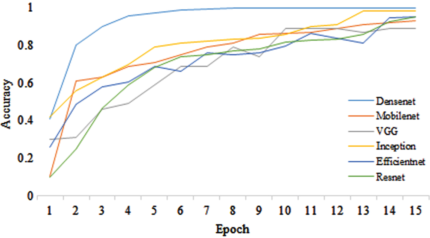
Comparison of training accuracy.

Fig. 6

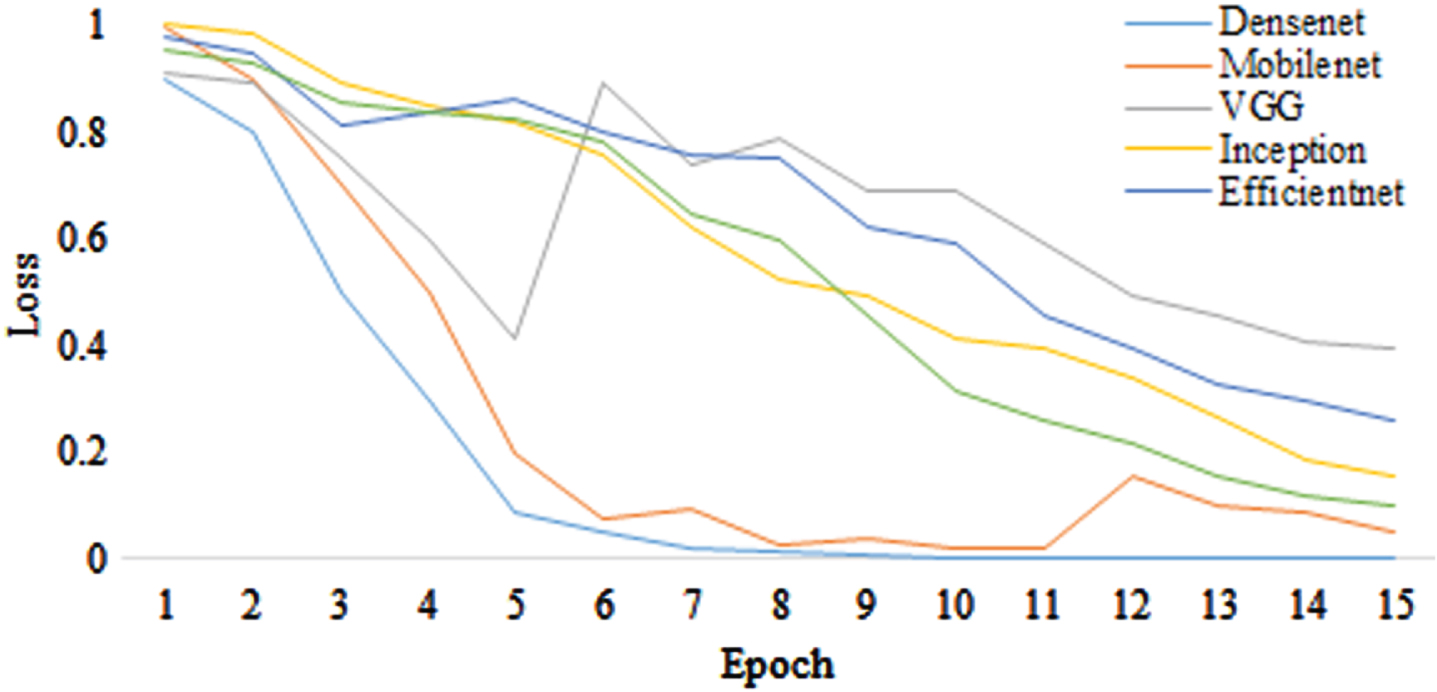
Comparison of training loss.

We impart an ensemble model of CNN based on deep features in this article. Pre-trained deep networks for disease detection are evaluated using six different models. DenseNet, MobileNet, EfficientNet, VGG19, ResNet and Inception are the names of these deep networks.

In this research study, we used the transfer learning technique to enhance pre-trained CNN models. The outcomes of the plant leaf disease identification clearly demonstrate the efficacy of the ESOS algorithm. We assessed the accuracy scores of fine-tuning for the DenseNet, MobileNet, EfficientNet, VGG19, ResNet, and Inception models to ascertain how transfer learning affected system performance. The outcomes of the modified models were then combined with the output of the ESOS algorithm. An ESOS algorithm was therefore given the deep characteristics of pre-trained CNN networks. Furthermore, Adam (stochastic gradient descent with momentum) learning was used as the deep network optimisation method. After 15 iterations, the training process was over. Table 2 contains the accuracy ratings that were obtained for this experimental study. Table 3 shows that the DenseNet design, among deep networks based on transfer learning, had the highest accuracy (98%), while the VGG19 architecture performed the worst (89%).

8 Conclusion

In this research, we proposed identifying plant diseases using deep CNN-based deep learning models. We assessed the effectiveness of deep learning-based feature extraction for detecting plant diseases using a range of models. The results show that deep learning algorithms are more effective than manual feature extraction techniques at extracting results. Faster calculation on the same hardware platform is the main advantage of the suggested paradigm because of higher performance with fewer parameters. Deep learning models are helpful for identifying diseases and in the field of agriculture. The simplest models to construct for transfer learning and fine-tuning are CNN models where the new assignment closely resembles the original. One of the elements that influences how well a model operates after being tweaked is the model optimisation approach. In this study, the performance of six enhanced CNN models with the Adam-trained ESOS algorithm is studied. The MoibileNet, DenseNet, EfficientNet, VGG19, ResNet, and Inception, CNN models are used in the study. Training accuracy curves are employed as statistical metrics for contrasting various models. DenseNet with an accuracy of 98%, precision of 84%, recall of 82%, and F1-score of 82% together with the ESOS optimization algorithm performs better than other CNN models and has somewhat greater accuracy when the number of epochs is set to 15. For forthcoming research, we plan to develop models that integrate a number of machine learning classifiers with deep learning networks. Additionally, methods for feature reduction will be researched in order to extract the most beneficial characteristics from the acquired deep data.

References

Sujatha

, Jyotir Moy Chatterjee , Jhanjhi

, Sarfraz Nawaz Brohi , Performance of deep learning vs machine learning in plant leaf disease detection, Microprocessors and Microsystems 80 (2021), 103615, ISSN 0141-9331, https://doi.org/10.1016/j.micpro.2020.103615

Jain

, Ramesh

AI based hybrid CNN-LSTM model for crop disease prediction: An ML advent for rice crop, 2021 12th International Conference on Computing Communication and Networking Technologies (ICCCNT), Kharagpur, India, 2021, pp. 1–7, doi: https://doi.org/10.1109/ICCCNT51525.2021.9579587.

Abbas Amreen , Sweta Jain , Mahesh Gour , Swetha Vankudothu , Tomato plant disease detection using transfer learning with C-GAN synthetic images, Computers and Electronics in Agriculture 187 (2021), 106279.

Sun Henan , Haowei Xu , Bin Liu , Dongjian He , Jinrong He , Haixi Zhang , Nan Geng , MEAN-SSD: A novel real-time detector for apple leaf diseases using improved light-weight convolutional neural networks, Computers and Electronics in Agriculture 189 (2021), 106379.

Hamdani Hamdani , Anindita Septiarini , Andi Sunyoto , Suyanto Suyanto , Fitri Utaminingrum , Detection of oil palm leaf disease based on color histogram and supervised classifier, Optik 245 (2021), 167753.

Pothen , Minu Eliz , Maya Pai

Detection of rice leaf diseases using image processing. In 2020 Fourth International Conference on Computing Methodologies and Communication (ICCMC), pp. 424–430. IEEE, 2020.

Mugithe , Pradeep Kumar , Rohit Varma Mudunuri , Rajasekar

, Karthikeyan

Image processing technique for automatic detection of plant diseases and alerting system in agricultural farms. In 2020 International Conference on Communication and Signal Processing (ICCSP), pp. 1603–1607. IEEE, 2020.

Venugopal

, Jayasankar

, Krishnaraj

, Venkatraman

, Prakash

N.B.

and Hemalakshmi

G.R.

, and , Multifactorial disease detection usingregressive multi-array deep neural classifier, IntelligentAutomation & Soft Computing 28(1) (2021).

Nawaz , Muhammad Amir , Rana Mudassar Rasool , Maryam Kausar , Amir Usman , Tanvir Fatima Naik Bukht , Rizwan Ahmad , Ahmad Jaleel , “Plant disease detection using internet of thing (IoT), International Journal of Advanced Computer Science and Applications 11(1) (2020).

10.

Mojjada , Ramesh Kumar , Kiran Kumar , Arvind Yadav

, Satya Vara Prasad

BVV

Detection of plant leaf disease using digital image processing, Materials Today: Proceedings (2020).

11.

Reddy , Ashish

, Megha Chandra Reddy

, Sujatha

Precision method for pest detection in plants using the clustering algorithm in image processing. In 2020 International Conference on Communication and Signal Processing (ICCSP), pp. 894–897. IEEE, 2020.

12.

Saleem

M.H.

, Potgieter

and Arif

K.M.

, Plant Disease Classification: A Comparative Evaluation of Convolutional Neural Networks and Deep Learning Optimizers, Plants (Basel) 9(10) (2020), 1319. doi: 10.3390/plants9101319. PMID: 33036220; PMCID: PMC7599959

13.

Abad-Segura , Emilio , Ana Batlles de la Fuente , Mariana-DanielaGonzalez-Zamar , Luis Jesús Belmonte-Ureña Effects of Circular Economy Policies on the Environment andSustainable Growth: Worldwide Research, Sustainability 12(14) (2020), 5792. https://doi.org/10.3390/su12145792.

14.

Tholkapiyan

, Aruna Devi

and Bhatt

, Performance Analysis of Rice Plant Diseases Identification and Classification Methodology, Wireless Pers Commun 130 (2023), 1317–1341. https://doi.org/10.1007/s11277-023-10333-3

15.

Hassan

S.M.

, Maji

A.K.

Deep feature-based plant disease identification using machine learning classifier, Innovations Syst Softw Eng (2022). https://doi.org/10.1007/s11334-022-00513-y.

16.

Turkoglu

, Yanikoglu

and Hanbay

, PlantDiseaseNet:convolutional neural network ensemble for plant disease and pestdetection, SIViP 16 (2022), 301–309. https://doi.org/10.1007/s11760-021-01909-2

17.

Haridasan

, Thomas

and Raj

E.D.

, Deep learning system for paddy plant disease detection and classification, Environ Monit Assess 195 (2023), 120. https://doi.org/10.1007/s10661-022-10656-x

18.

Prasath

, Sreemathy

, Krishnaraj

, Vigneshwaran

Analysis of Crop Yield Prediction Using Random Forest Regression Model. In: So-In, C., Londhe, N.D., Bhatt, N., Kitsing, M. (eds) Information Systems for Intelligent Systems. Smart Innovation, Systems and Technologies, vol 324. Springer, Singapore. (2023) https://doi.org/10.1007/978-981-19-7447-2_22.

19.

Adesh Panchal

, Subhash Chandra Patel , Bagyalakshmi

, Pankaj Kumar , Ihtiram Raza Khan , Mukesh Soni , Image-based Plant Diseases Detection using Deep Learning, Materials Today: Proceedings 80(Part 3) (2023), 3500–3506, ISSN 2214-7853, https://doi.org/10.1016/j.matpr.2021.07.281

20.

Binnar

, Sharma

Plant Leaf Diseases Detection Using Deep Learning Algorithms. In: Doriya, R., Soni, B., Shukla, A., Gao, XZ. (eds) Machine Learning, Image Processing, Network Security and Data Sciences. Lecture Notes in Electrical Engineering, vol 946. Springer, Singapore (2023). https://doi.org/10.1007/978-981-19-5868-7_17

Enhanced symbiotic organism search optimization algorithm for plant disease classification

Abstract

Keywords

1 Introduction

2 Literature survey

4.1 Pseudocode for ESOS algorithm

5 Deep learning architectures

5.1 DenseNet

Table 2 Exhaustive deterioration of model output parameters Model Accuracy (%) Loss (%) Precision Recall F1-score DenseNet 98 2 84 82 82 MobileNet 93 7 80 80 79 EfficientNet 95 18 78 77 76 VGG19 89 11 72 71 71 ResNet 95 5 76 75 74 Inception 96 4 74 73 72

References

Table 2
Exhaustive deterioration of model output parameters

Model Accuracy (%) Loss (%) Precision Recall F1-score

DenseNet 98 2 84 82 82

MobileNet 93 7 80 80 79

EfficientNet 95 18 78 77 76

VGG19 89 11 72 71 71

ResNet 95 5 76 75 74

Inception 96 4 74 73 72