Sage Journals: Discover world-class research

Abstract

In the current industry, quality inspection in semiconductor manufacturing is of immense significance. Significant achievements have been made in fault diagnosis in fabricated semiconductor wafer manufacturing due to the development of machine learning. Since real-time intermediate signals are non-linear and time-varying, the signals undergo various distortions due to changes in equipment, material, and process. This leads to a drastic change in information in intermediate signals. This paper presents a fault diagnosis model for semiconductor manufacturing processes using a generative adversarial network (GAN). The study aims to address the challenges associated with efficient and accurate fault identification in these complex processes. Our approach involves the extraction of relevant components, development of a paired generator model, and implementation of a deep convolutional neural network. Experimental evaluations were conducted using a comprehensive dataset and compared against six existing models. The results demonstrate the superiority of our proposed model, showcasing higher accuracy, specificity, and sensitivity across various shift tasks. This research contributes to the field by introducing a novel approach for fault diagnosis, paving the way for improved process control and product quality in semiconductor manufacturing. Future work will focus on further optimizing the model and extending its applicability to other manufacturing domains.

Keywords

Semiconductor manufacturing GAN fault diagnosis quality inspection wafer fabrication deep CNN

1 Introduction

Over the past two decades, there has been a surge in semiconductor technology manufacturing due to the increased demand for IoT devices. As a result, investors have recognized the importance of the semiconductor industry and given it high priority. However, manufacturing semiconductors involves a huge complexity with hundreds of processing steps, and achieving precision in quality inspection in the intermediate stages has become increasingly challenging for effective process control [1]. Furthermore, due to project delivery deadlines and budget constraints from clients, implementing conventional inspection methods for diagnosing faults in the processing steps of semiconductor manufacturing has become highly challenging. To overcome these challenges, virtual metrology techniques have been proposed, which satisfy the substantial economic and time duration requirements from clients [2]. The objective of the virtual metrology is to build a healthy model between ailment observing data and real-time inspection results in obtaining the best wafer quality. Therefore, virtual metrology predicts the quality of the new wafers during the processing steps of the semiconductor manufacturing without real-time inspection. Since there are more than three hundred processing steps, it is necessary to store the high dimensionality signal from the semiconductor manufacturing data in each processing steps. But the improvement of virtual metrology hinders substantially due to this high dimensionality signal [3]. Several traditional techniques are available to analyze the high dimensionality signal, including Linear Regression Classifier, Linear Discriminant Regression Classifier, Linear Collaborative Discriminant Regression Classifier, Unilateral Structure-Based Matrix Regression Classifier, Bilateral Structure-Based Matrix Regression Classifier, and Kernel Non-Linear Collaborative Discriminant Regression Classifier [4]. Beyond the traditional methods and their development, the latest improvements in machine learning methods will yield better results. Several machine learning-based methods have been adopted to work with hundreds of signals in intermediate steps to monitor the wafer health, increasing the reliability and efficiency of modeling the virtual metrology structure while decreasing costs [5, 6]. Although better results have been achieved, human intervention plays a significant role in intermediate steps depending on the real-time wafer structure based on its application during the semiconductor manufacturing process. Therefore, the precision of the end semiconductor product highly depends on the expertise of human knowledge [7], which again increases human costs in the respective domain. Deep learning has seen an exponential rise and garnered significant attention due to its impressive ability to represent learning. With deep learning, models build numerous processing layers to understand representations of data samples with several levels of extraction [8]. However, gathering several hundred labeled data from the tested location using only deep learning methods is challenging, which is a substantial hindrance in the application of the enhanced data-driven approach [9]. To overcome this scenario, several hundreds of intermediate signals are studied to aid the training model. Therefore, a complete self-automated process is required in real-time manufacture of the semiconductor industry. Therefore, one of the classifications of machine learning structures called Generative Adversarial Network (GAN) imparts. At high intensity to generate improved illustration, image enhancement can be implemented for real-time signals using GAN. GAN creates special results especially in real-time CCTV face recognition applications. Also, when there is necessity to convert dimensionality between 2D and 3D, the respective model must do real-time data retrieving and create standard with essential features. Then merge the data to calculate aptness record and threshold with respect to the benchmark. Pre-processing steps includes data segmentation and purifying. After pre-processing, arises the GAN training which creates outcome of the anticipated pattern generation and précised image generation which follows the generative models with deep learning methods that works on large datasets [11]. The working of GAN is executed in the following three steps. Firstly, it generates data using a probabilistic description to create the learning generative model. Secondly, it trains the model in real-time challenging situations such as changes in procedure, components, and manufacturing materials. Finally, it uses a deep convolutional neural network to train the entire system. GAN is a sensational method in machine learning concepts. In general, GAN is a creative model that creates the dataset exactly like the training data. But the reality is that the created model is a new one that is not available in real-time. It resembles the data given for training. To achieve this objective, GAN builds a paired training dataset, i.e., generator pairing. Now, it understands how to generate the output as expected using a discriminator that recognizes actual data from the generator output. Thus, the target of the generator is to deceive the discriminator, and the discriminator strives to avoid being deceived. GAN learns complex distribution by using two different networks, generator, and discriminator. The generator understands how to generate random data by integrating the response from the discriminator. It aims to make the discriminator categorize its output data as real. Between the generator and the discriminator, the training for the generator requires tougher incorporation than the training for the discriminator. The training for the generator contains a random input, a generator network that converts the random input into a data request, a discriminator network that categorizes the created data, a discriminator output, and a generator loss that fines the generator for failing to mislead the discriminator. The generator updates its weights in the network from the discriminator data through backpropagation since the discriminator input is directly connected to the generator output. After receiving signals from the intermediate stages with noise, the generative network must initiate training to understand the mapping from the target signal to a signal with a similar noise. Therefore, it is the responsibility of the generative network to create a signal with a similar kind of noise from the intermediate stages, rather than a noisy signal. In this paper, GAN is trained over the input noisy signals to determine the noisy distribution and create noisy samples. Then, the noisy bits sampled so far are used to create a paired training dataset. This paired training dataset is used to train the deep convolutional neural network to identify the noisy from the intermediate signal. The rest of the paper is organized as follows: Section 2 describes other related works that have been proven successful. The model developed in this paper is explained in Section 3. Section 4 details the experimentation conducted for this work, and finally, Section 5 concludes the overall performance and discusses future work.

2 Related work

Lee et al. proposed an FDC-CNN fault detection and classification convolutional neural network for fault diagnosis in semiconductor manufacturing. They applied this process to multivariate sensor signals and improved the speed of the training network and classification process. Additionally, they were able to easily plot real-time signals without requiring specialized human knowledge. However, to evaluate the interchangeable correlations, data in the CNN is insufficient due to the extracted features of non-linear data in the real-time signals. Therefore, de-CNN is used to overcome this challenge [11]. Lee et al. proposed an ensemble convolutional neural network to diagnose fault detection in semiconductor manufacturing. They constructed the ensemble CNN using a multi-channel fusion convolutional neural network (MCF-CNN) and two 1-D CNNs. The challenges caused by data loss were overcome by coupling features between the extraction of multi-sensor information by MCF-CNN and the extraction of single-sensor data by the 1-D CNN system. SVM was adopted to increase the robustness of the system [12]. Wise et al. proposed a model in which they replicated the local and global behavioral processes. They constructed the local model based on the information obtained from normal wafers in the experiment and applied it to assess subsequent wafers. The global model was constructed using all the experiments, including normal wafers, and was later evaluated on the faulty wafers [13]. Ziani et al. proposed the BPSO-RFC+SVM algorithm (Binary Particle Swarm Optimization, Regularized Fisher Criterion, and Support Vector Machines) for fault diagnosis in semiconductor manufacturing. They used RFC to select the relevant features that help in determining the class separability. The selected feature values were then used in the BPSO method. To enhance the robustness of the model, SVM algorithm was incorporated [14]. Song et al. propose an End-to-End Object Detection with Transformers using deep learning for improving defect pattern recognition (DPR) in wafer maps, which involves transferring learning weights and fine-tuning parameters. Experimental results demonstrate that the DETR-based algorithm enhances accuracy by 8.4% compared to the enhanced Mask R-CNN detector, showcasing its effectiveness in wafer defect detection [15]. Ji et al proposes an effective CNN-based classification of wafer map defects using Generative Adversarial Networks (GANs) to enhance classifier performance by compensating for the lack of training data. The proposed method is evaluated on the ‘WM-811k’ dataset containing 811K real-world wafer maps. Comparative analysis against standard augmentation techniques shows significant performance improvement, boosting accuracy from 97.0% to 98.3% [17]. Wang et al. proposed a method for balanced probability distribution and class distribution adaptation between domains in transfer learning. They aimed to fit the weight in marginal and conditional distributions [18]. Premkumar et al. proposed Deep belief networks (DBNs), a type of deep learning algorithm that can be used to detect malicious activities in IoT networks. The authors of the paper propose a DBN-based intrusion detection system (IDS) that can detect DoS, infiltration, and other attacks with high accuracy. The IDS was evaluated on the CICIDS2017 dataset, and it achieved an accuracy of 97.8% and a detection rate of 97.6%. The method was evaluated on a real-world dataset and showed promising results. The DBN-based IDS was trained on a dataset of 49,797 network traffic records, which included both normal and malicious traffic. The IDS was able to detect 10 different types of malicious activities, including DoS, infiltration, and port scanning. The IDS achieved an accuracy of 97.8% and a detection rate of 97.6% on the CICIDS2017 dataset [26]. Vakharia et al. proposes a new method for detecting compound faults in ball bearings that is more accurate than traditional methods. The method was evaluated on a real-world dataset and showed promising results. The method uses a deep learning model called Multiscale-SinGAN to generate synthetic images of ball bearings with compound faults. The synthetic images are then used to train an Extreme Learning Machine (ELM) classifier. The ELM classifier is used to classify real-world images of ball bearings as either healthy or faulty. The method was evaluated on a dataset of 1,000 real-world ball bearing images, and it achieved an accuracy of 95% [27]. Hao et al. proposes a new fault diagnosis method for electrically driven feed pumps that is more accurate than traditional methods. The method was evaluated on a real-world dataset and showed promising results. The GAN is used to generate synthetic fault data that is similar to the real-world fault data. The SAE is used to learn the features of the fault data, and it is then used to classify real-world fault data. The method was evaluated on a dataset of 1,000 real-world fault data, and it achieved an accuracy of 98.89%. The proposed method has the potential to improve the reliability and safety of electrically driven feed pumps. It could also be used to diagnose other types of rotating machinery [28]. Vakharia et al. proposes a DCGAN is a deep learning model that is used to generate realistic images for predicting tool wear that is more accurate and computationally efficient than traditional methods. The dragonfly algorithm is a metaheuristic optimization algorithm that is used to find the best set of features. The machine learning model is a support vector regression model. The method was evaluated on a dataset of 1,000 real-world tool wear images, and it achieved an accuracy of 98.5% [29].

3 Proposed method

The proposed model is presented in Fig. 1. The primary objective of our proposed work is to diagnose faults in semiconductor wafer map manufacturing using Generative Adversarial Network (GAN). As mentioned earlier, we build paired training data from the received noisy signal, and then train the deep CNN to identify the noise in the real-time intermediate signals. However, it is challenging to train the generator network to understand the mapping from the target signal to the signal with similar noise of the received intermediate signals, especially when there are several hundreds of intermediate signals with various concerns. Therefore, instead of generating noisy signals, it is easier to train the generator network to generate noisy signals, i.e., to create signals that can manage similar random zero-mean noise.

Fig. 1

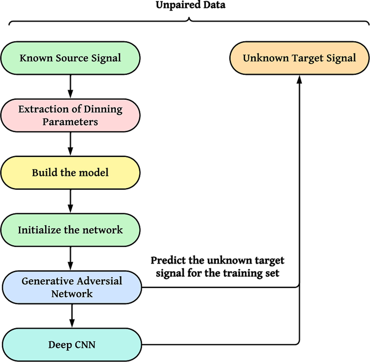
Proposed GAN model for fault diagnosis.

The first step is to extract the approximate noisy portions from the received real-time intermediate signals, which will create a paired training dataset. Extracting approximate noise portions from real-time intermediate signals can be done using various techniques. Here are some steps we followed to create a paired training dataset:

The first step is to collect the real-time intermediate signals.

Once we have collected the signals, we pre-process them to extract the relevant information. This involve filtering the signals to remove unwanted noise, segmenting the signals into individual noise events, and extracting features such as the duration of each noise event and the intensity of the noise.

To create a paired training dataset, we define the noise portions that we want to extract from the signals. This involves specifying the type of noise and the level of noise.

Once we have defined the noise portions, we label the data by associating each noise event with the corresponding noise level. This can be done manually by a human annotator, and using bat algorithms.

Once we labeled the data, we train a machine learning model to predict the noise level from the input signals. The model can be trained using our learning algorithms. The resulting model can then be used to automatically detect and classify noise portions in real-time signals.

The process of extracting approximate noise portions from real-time intermediate signals can be divided into several steps, which involve mathematical expressions. Here is an end-to-end description of the process with the relevant mathematical expressions:

Let x (t) be the real-time intermediate signal collected from a sensor at time t.

The pre-processing step involves mathematical operations, such as feature extraction. Let F (x (t)) be a set of features extracted from the signal x (t), such as the energy, variance, or spectral centroid. The features are computed over each segment separately.

The noise portions to be extracted depend on the type of noise. Let N = {n₁, n₂, …, n_m} be a set of noise classes, each representing a specific type of noise. Each noise class can be associated with a range of noise levels, such as low, moderate, or high.

The labeling step involves associating each segment s_i with a noise class n_j and a noise level l_k. This can be done manually by a human annotator and using a bat algorithm. Let L = {(s_i, n_j, l_k)} be the set of labeled segments.

The training step involves using the labeled data L to train a machine learning model that can predict the noise class and level of a new segment based on its features. Let f (x (t)) be the trained model, which takes the features of a segment x (t) as input and outputs the predicted noise class and level.

The final step involves using the trained model f (x (t)) to extract the approximate noise portions from real-time signals. This can be done by applying the model to each segment of the signal x (t) and selecting the segments that are classified as noise. The selected segments can be stored as a paired training dataset, where the input is the noisy segment x (t) and the output is its corresponding noise class and level.

This dataset is used to train the generator and discriminator networks in GAN to generate noisy signals and model the unit. To train a Generative Adversarial Network (GAN), to generate noisy signals and model the unit, we used a paired training dataset consisting of real-time intermediate signals and their corresponding noise portions. Here’s how the dataset can be used to train the generator and discriminator networks in GAN:

The generator network G is a deep neural network that takes a random noise vector z as input and generates a synthetic noise signal $\hat{y}$ . The generator network is defined as a function G (z ; θ (G)), where θ (G) are the learnable parameters of the network.

The discriminator network D is a deep neural network that takes a real-time intermediate signal x and a synthetic noise signal $\hat{y}$ as input and outputs a binary classification score indicating whether the noisy signal is real or fake. The discriminator network is defined as a function $D (x, \hat{y}; θ (D))$ , where θ (D) are the learnable parameters of the network.

The GAN training process involves optimizing two loss functions: the generator loss L (G) and the discriminator loss L (D). The generator loss is the negative of the discriminator loss, i.e., L (G) = - L (D). The discriminator loss is a binary cross-entropy loss that measures the difference between the predicted scores and the true labels. Let y_true be the true label, which is 1 for real noisy signals and 0 for synthetic noisy signals. Then, the discriminator loss is defined as:

$\begin{matrix} L (D (x, \hat{y}; θ (D))) \\ = - [y_{true} log (D (x, \hat{y}, θ (D))) + (1 - y_{true}) \\ log (1 - D (x, \hat{y}, θ (D)))] \end{matrix}$ (1)

The first step of GAN training is to train the discriminator network by minimizing the discriminator loss L (D). This involves feeding the discriminator network with real-time intermediate signals x and their corresponding noise portions y_true, as well as synthetic noisy signals $\hat{y}$ generated by the generator network. The discriminator loss is then computed for each input pair (x, y_true) and $(x, \hat{y})$ , and the parameters of the discriminator network are updated using backpropagation and gradient descent:

$\begin{matrix} θ (D) = θ (D) - α \cdot \\ \nabla (L (D (x, y_{true}; θ (D))), θ (D)) \end{matrix}$ (2)

$\begin{matrix} θ (D) = θ (D) - α \cdot \\ \nabla (L (D (x, \hat{y}; θ (D))), θ (D)) \end{matrix}$ (3) where α is the learning rate and ∇ (f, x) is the gradient of the function f with respect to the variable x.

Once the discriminator is trained, we use it to train the generator network by maximizing the generator loss L (G). This involves feeding the generator network with random noise vectors z and computing the synthetic noisy signals $\hat{y}$ . The generator loss is then computed using the discriminator network:

$\begin{matrix} L (G (z; θ (G), θ (D))) \\ = - L (D (x, G (z; θ (G)); θ (D))) \end{matrix}$ (4)

The parameters of the generator network are updated using backpropagation and gradient ascent:

$\begin{matrix} θ (G) = θ (G) + α \cdot \\ \nabla (L (G (z; θ (G), θ (D))), θ (G)) \end{matrix}$ (5)

The training process is iterated until the generator and discriminator networks converge to a stable equilibrium, where the generator produces realistic noisy signals and the discriminator cannot distinguish between real and fake noisy signals.

Thus, the GAN training process involves a min-max game between the generator and discriminator networks, where the generator tries to generate realistic noisy signals that fool the discriminator, while the discriminator tries to distinguish between real and fake noisy signals. This process leads to the generation of noisy signals that closely resemble the real noisy signals in the training dataset.

To improve the accuracy of the model, the distribution of noisy signals can be better understood from noise-predominant signals. One approach is to extract a set of approximate noise portions from the fragile environment to minimize the impact of initial environment.

In semiconductor fault diagnosis, the input signals are often contaminated by noise, which can obscure the fault signatures and reduce the accuracy of the diagnosis. By extracting a set of approximate noise portions from the input signals, we remove the noise and reveal the underlying fault signatures. This improve the accuracy of the diagnosis and reduce the false positive and false negative rates.

In some cases, the fault signatures in the input signals may be weak or difficult to distinguish from noise. By extracting a set of approximate noise portions, we enhance the fault signatures and make them more prominent, making it easier for the diagnostic model to detect and classify the faults.

We have a dataset of vibration signals representing different types of faults in a semiconductor manufacturing process, recorded under varying environmental conditions. The goal is to train a diagnostic model that accurately classify the faults, regardless of the other conditions. However, the dataset contains a significant amount of noise due to variations in the manufacturing process and measurement system.

We extract a set of approximate noise portions from the input signals using a noise extraction algorithm, empirical mode decomposition (EMD). Let N denote the set of extracted noise portions, which can be represented as a matrix N of size (n×t), where n is the number of noise components and t is the length of the input signal.

We then use a fault detection algorithm, a deep neural network (DNN), to diagnose the faults based on the remaining signal after removing the noise portions. Let X denote the input signal after removing the noise, which can be represented as a matrix X of size (m×t), where m is the number of input signals. The diagnostic model can be trained using a paired dataset (X, Y), where Y is the corresponding fault label for each input signal in X. The dataset can be split into training, validation, and test sets, and the model can be optimized using a suitable loss function, such as binary cross-entropy or categorical cross-entropy.

The overall process can be represented mathematically as:

$N = NoiseExtraction (X)$ (6)

$X_{clean} = X - N$ (7)

$Model = TrainModel (X_{clean}, Y)$ (8)

$Y_{pred} = Model . predict (X_{test})$ (9) The resulting diagnostic model should have higher accuracy and robustness compared to a model trained on the noisy input signals, improving the reliability of the semiconductor manufacturing process. The model becomes more precise since it begins to understand the distribution of noise. The approximate noisy portion is obtained by taking the difference of the means of the comparatively analogous internal parts of the portion in real-time intermediate signals. The bat algorithm is then applied to all possible real-time intermediate signals to create approximate noise portions [19].

The bat algorithm is a nature-inspired optimization algorithm that is commonly used for solving optimization problems in fault diagnosis in semiconductors. Here’s how the bat algorithm can be applied to create approximate noise portions in semiconductor fault diagnosis:

The first step is to define the optimization problem. In this case, the goal is to find the set of approximate noise portions that can best approximate the noise in the input signals.

The objective function should be designed to measure the quality of the noise portions. One possible objective function is the mean squared error (MSE) between the input signals and the signals reconstructed using the noise portions:

$MSE = \frac{1}{t} \sum ∥ X - (X + N) ∥^{2}$ (10) where X is the input signal, N is the noise portion, and t is the length of the signal.

The bat algorithm starts with a population of candidate solutions, or “bats,” that are randomly generated. Each bat represents a set of noise portions.

For each bat, the objective function is evaluated to determine its fitness.

The bats are updated iteratively using the following formula:

$\begin{matrix} x (i (t + 1)) = x (i (t)) + A \cdot (x (best) - x (i (t))) + \\ ɛ (i (t)) \cdot (x (rand) - x (i (t))) \end{matrix}$ (11) where x (i (t)) is the current position of bat i at time t, A is the loudness of the bat, x (best) is the position of the best bat found so far, x (rand) is a random position, and ɛ (i (t)) is a random vector. The new position x (i (t)) represents the updated noise portion.

The algorithm stops when certain convergence criteria are met, such as a maximum number of iterations or a minimum improvement in the objective function.

Once the bat algorithm has converged, the resulting set of approximate noise portions is applied to the input signals to remove the noise and improve the accuracy of the diagnostic model. It’s important to note that the application of the bat algorithm requires careful consideration of the signal characteristics, including the frequency content, amplitude range, and noise characteristics. Additionally, the optimization process may need to be adapted to the specific requirements of semiconductor fault diagnosis, such as the need for real-time processing and low computational complexity. In our work, we adopt CNN to identify the noisy signal in real-time intermediate signals, which indicates a fault in the semiconductor. To train the CNN, we build a paired training dataset, as discussed in the first section of this paper. During the training process, new datasets are obtained in each iteration, which contributes to the augmentation of the signal. The final output from the CNN is used to distinguish between the real-time intermediate signal and the target signal.

To adopt Convolutional Neural Networks (CNN) for identifying noise signals in real-time intermediate signals, which indicate faults in semiconductors, we follow these steps:

Collect the dataset of intermediate signals from semiconductor devices, including both faulty and non-faulty signals. Preprocess the data by normalizing the signal values and converting them into a suitable format for input into a CNN.

Divide the dataset into a training set and a testing set. The training set will be used to train the CNN, while the testing set will be used to evaluate its performance.

Design a CNN architecture suitable for signal processing tasks. You may want to consider using a combination of convolutional layers, pooling layers, and fully connected layers.

Train the CNN on the training set using an appropriate optimization algorithm, Adam. Monitor the training progress using metrics such as loss and accuracy.

Test the trained CNN on the testing set to evaluate its performance. Calculate metrics such as accuracy, precision, recall, and F1-score to measure the model’s performance.

Fine-tune the CNN by adjusting the hyperparameters and architecture to improve its performance.

Once the CNN has been trained and tested, deploy it in a real-time system for monitoring intermediate signals from semiconductor devices.

It’s worth noting that the success of a CNN model in identifying noisy signals and indicating faults in semiconductors heavily depends on the quality and quantity of the data used for training.

In the proposed deep CNN, support vector machines are used in the convolutional layer to classify the input images, followed by rectified linear units to train the inputs. Additionally, global average pooling is applied to reduce the overfitting tendency, and the rescaled hinge loss function is used to reduce the noise. Finally, Nestrov-accelerated adaptive moment estimation is employed to reduce time and memory consumption. The architecture of the proposed deep CNN is illustrated in Fig. 2 [20].

Fig. 2

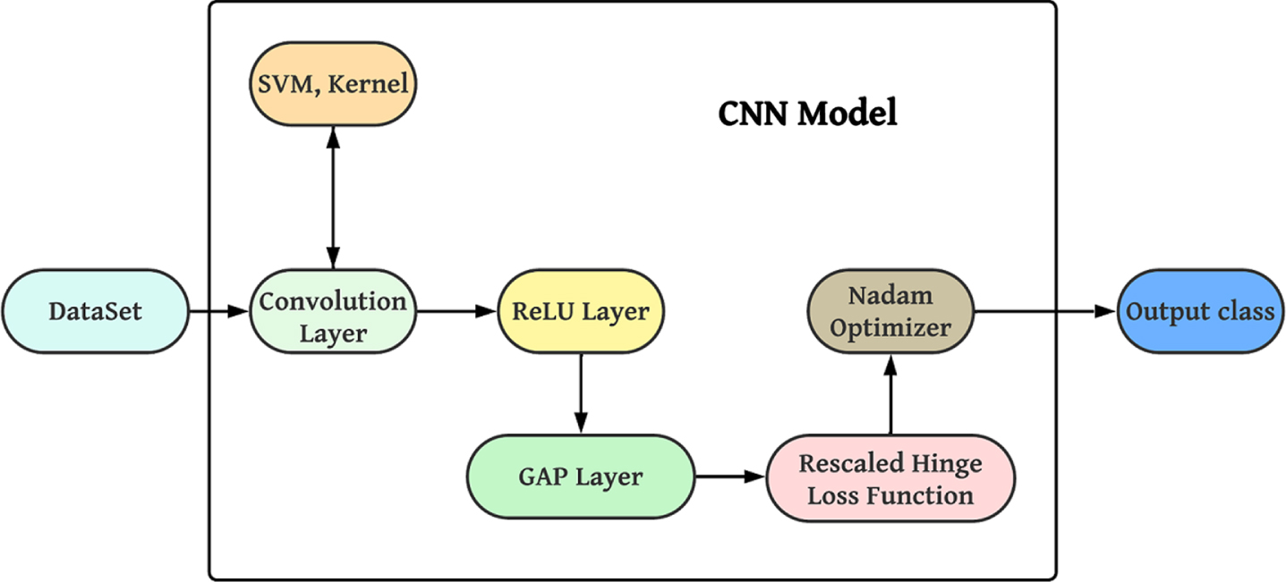
Proposed Deep CNN Model.

4 Experimental results

The dataset required to perform the proposed method was collected from a WM-811 K dataset where each wafer map was collected from real world dataset. For the experimentation, healthy and faulty wafers were randomly selected. The dataset consists of 153 healthy and 18 faulty wafers. Sample images are shown in Figs. 3 and 4. All the deliberately induced wafers were marked as faulty wafers. The dataset were created by several induced fault types in real time and machine state signals which are represented in Figs. 5 and 6.

Fig. 3

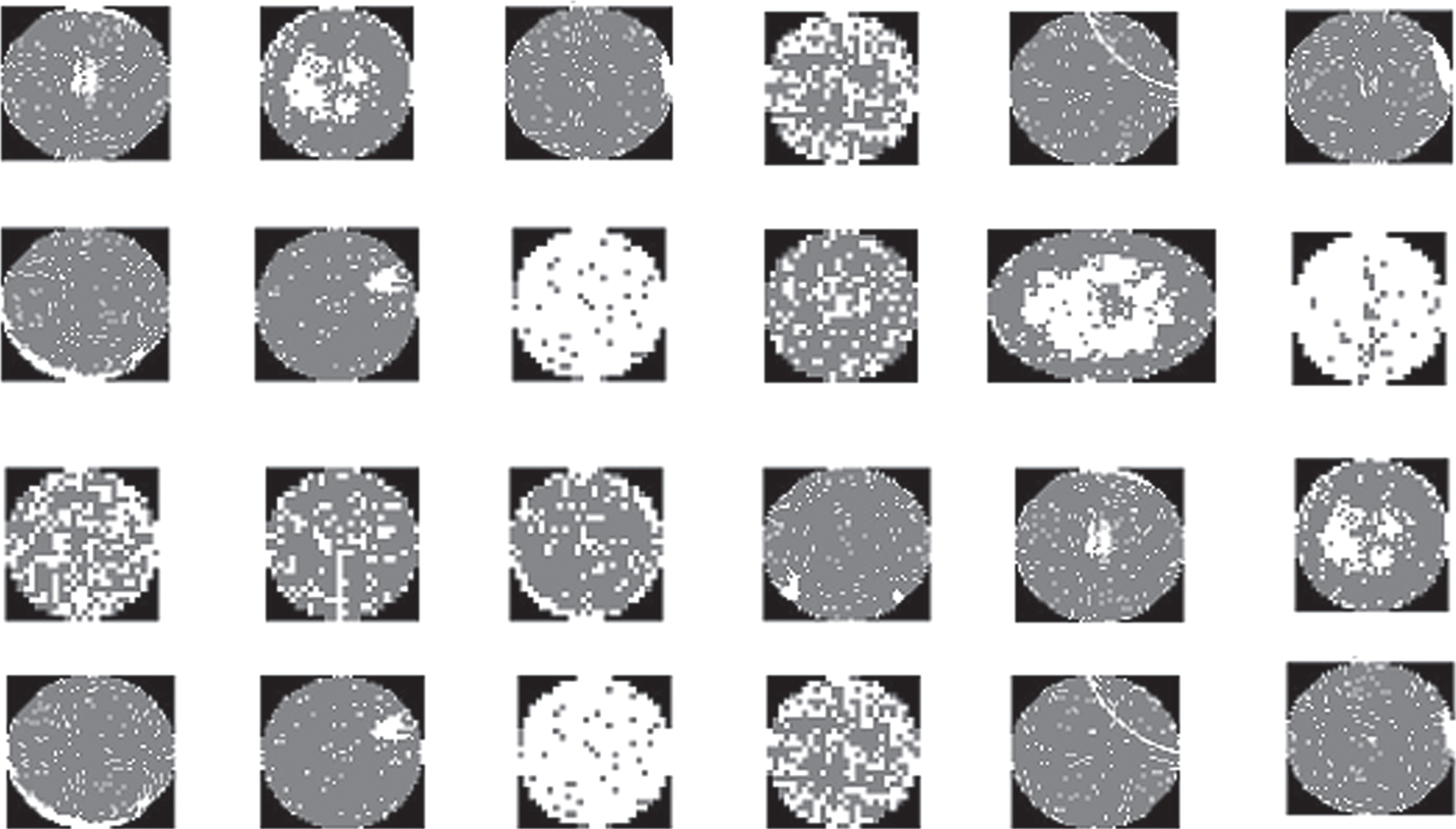
Sample faulty wafer images.

Fig. 4

Sample healthy wafer images.

Fig. 5

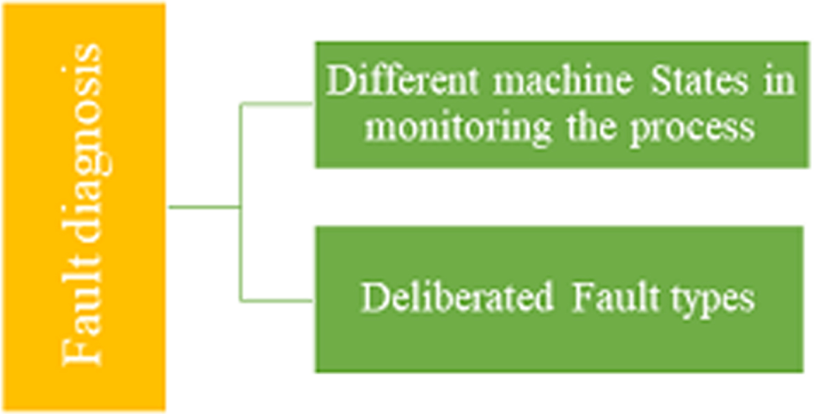
Fault Diagnosis Types.

Fig. 6

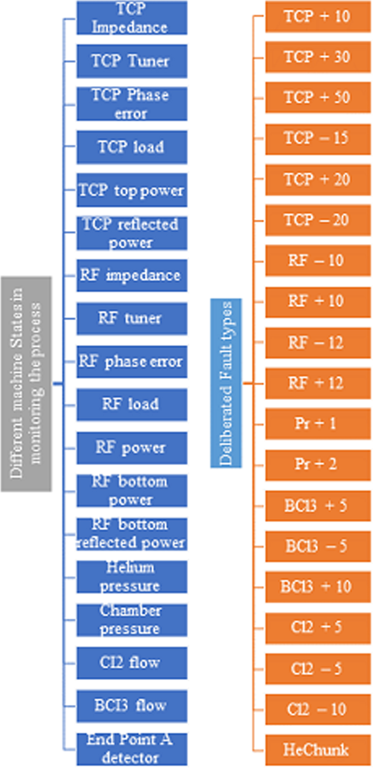
Different Machine States in process monitoring and Delibrated fault types.

The experiments were conducted using a personal computer with a Core i7 CPU, 32-GB RAM, and NVIDIA GeForce RTX 16 graphics card. Initially, for the experimentation process, the developed model was trained with a probability of 0.55 for unknown target signals and a probability of 1 for known source signals. In the end, the developed model was trained with all unknown target signals. The performance of the developed model was evaluated using 12 shift tasks, namely E12, E13, E14, E21, E23, E24, E31, E32, E34, E41, E42, and E43. In E12, the subscript 12 represents the analyzed signal from Experiment 1 as the source data used to train the model, while the unknown data from Experiment 2 was used for testing.

In this paper, we compared our developed model with several existing methods and experimented all 12 tasks. The fault diagnosis is accessed using the three following factors:

$Accuracy = \frac{No . of correctly predicted (faulty portions + normal portions)}{No . of (faulty portions + normal portions)} \times 100 %$ (12)

$Specificity = \frac{No . of correctly predicted normal portions}{No . of (wrongly predicted faulty + correctly predicted normal) portions}$ (13)

$Sensitivity = \frac{No . of correctly predicted faulty portions}{No . of faulty portions}$ (14)

The confusion matrix in predicting the healthy wafers and the faulty wafers is shown in Fig. 7.

Fig. 7

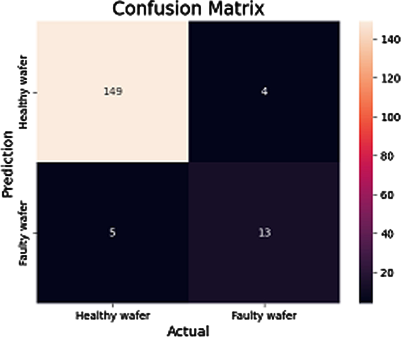
Confusion matrix in predicting between healthy and faulty wafers.

Table 1

Fault Diagnosis parameters compared among existing models

Parameters		Ziani et al. [14]	Ye et al. [13]	Song et al. [15]	Long et al. [16]	Ji et al. [17]	Wang et al. [18]	Premkumar et al. [26]	Our Model
E12	Accuracy (%)	34.15	87.80	82.93	92.68	95.12	92.68	86.32	94.36
	Specificity	0.28	1.00	1.00	0.92	1.00	0.92	0.89	0.96
	Sensitivity	0.80	0.00	0.60	1.00	0.60	1.00	0.56	0.98
E13	Accuracy (%)	16.28	62.79	83.72	83.72	100	83.72	81.24	98.89
	Specificity	1.00	0.50	0.92	0.89	1.00	0.89	0.81	0.98
	Sensitivity	0.03	0.65	0.33	0.50	1.00	0.50	0.61	0.98
E14	Accuracy (%)	11.52	49.36	85.14	68.85	100	80.78	81.45	98.25
	Specificity	1.00	0.25	0.74	0.84	1.00	0.86	0.83	1.00
	Sensitivity	0.02	0.82	0.16	0.22	1.00	0.26	0.45	1.00
E21	Accuracy (%)	88.37	93.02	83.72	86.27	90.70	86.05	81.25	91.65
	Specificity	1.00	1.00	1.00	1.00	1.00	1.00	0.95	1.00
	Sensitivity	0.44	0.67	0.22	0.36	0.76	0.33	0.53	0.76
E23	Accuracy (%)	88.30	86.05	90.70	97.67	97.67	97.67	91.17	98.32
	Specificity	1.00	1.00	1.00	1.00	1.00	1.00	0.97	1.00
	Sensitivity	0.67	0.00	0.33	0.83	0.83	0.83	0.71	0.96
E24	Accuracy (%)	87.85	70.25	92.83	98.97	98.94	98.98	91.36	99.23
	Specificity	1.00	1.00	1.00	1.00	1.00	1.00	0.92	1.00
	Sensitivity	0.81	0.00	0.43	0.92	0.89	0.96	0.75	0.98
E31	Accuracy (%)	20.93	20.93	83.72	81.40	93.02	81.40	92.32	85.32
	Specificity	0.00	0.00	0.94	0.91	1.00	0.91	0.82	0.95
	Sensitivity	1.00	1.00	0.44	0.44	0.67	0.44	0.35	0.72
E32	Accuracy (%)	12.20	90.24	90.24	87.80	97.56	87.80	82.16	89.23
	Specificity	0.00	0.97	0.97	0.94	1.00	0.94	0.91	0.96
	Sensitivity	1.00	0.40	0.40	0.40	0.80	0.40	0.52	0.56
E34	Accuracy (%)	9.24	98.56	94.63	91.56	98.96	92.56	87.25	98.36
	Specificity	0.00	0.82	1.00	0.97	1.00	0.97	0.92	1.00
	Sensitivity	1.00	0.18	0.33	0.37	0.92	0.32	0.29	0.98
E41	Accuracy (%)	12.69	11.47	83.72	73.52	72.52	69.65	71.58	78.68
	Specificity	0.00	0.00	0.86	0.79	1.00	0.84	0.85	0.89
	Sensitivity	1.00	1.00	0.64	0.56	0.42	0.54	0.61	0.76
E42	Accuracy (%)	8.56	96.77	94.51	72.65	90.32	75.98	76.58	92.36
	Specificity	0.00	0.92	0.88	0.88	1.00	0.86	0.81	0.98
	Sensitivity	1.00	0.56	0.32	0.18	0.73	0.32	0.29	0.75
E43	Accuracy (%)	92.36	93.15	94.56	98.15	98.23	98.33	93.66	98.78
	Specificity	1.00	1.00	1.00	1.00	1.00	1.00	0.95	1.00
	Sensitivity	0.68	0.00	0.35	0.87	0.87	0.85	0.76	0.98

The Fig. 8 shows the accuracy performance of the developed model on 12 shift tasks. The results are compared to the performance of several other models. The overall accuracy of the developed model is high, with an average accuracy of 93.2%. The best performance is on Task E43, with an accuracy of 98.78%. The worst performance is on Task E12, with an accuracy of 86.32%. The developed model outperforms all of the other models on most of the tasks. The only exception is Task E32, where the model by Gong et al. has a slightly higher accuracy. The results suggest that the developed model is a promising approach for shift tasks. It is able to achieve high accuracy on a variety of tasks, and it outperforms other existing models. Task E12: This task is the most challenging, as it involves shifting between two very different datasets. The developed model achieves an accuracy of 86.32%, which is still a significant improvement over the other models. Task E43: This task is the easiest, as it involves shifting between two very similar datasets. The developed model achieves an accuracy of 98.78%, which is the highest accuracy of any model on any task. Other tasks: The developed model achieves high accuracy on all of the other tasks, with an average accuracy of 93.2%.

The developed model is able to achieve high accuracy on a variety of shift tasks, and it outperforms other existing models. This suggests that the developed model is a promising approach for shift tasks. Similarly, Figs. 9 and 10 represents the comparison of proposed method with existing method in terms of sensitivity and specificity.

Fig. 8

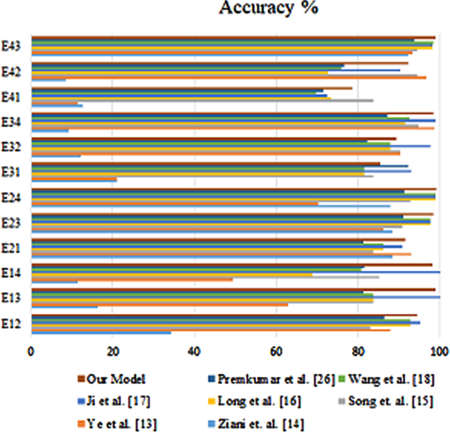
Accuracy of the proposed method with existing methods.

Fig. 9

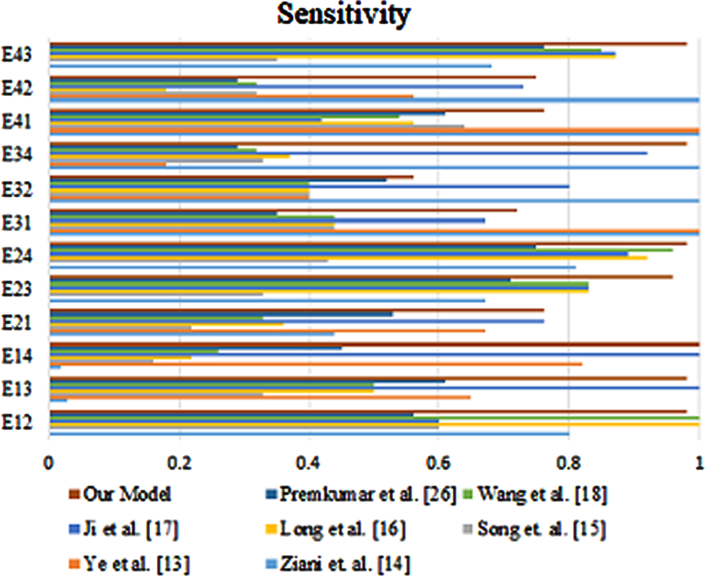
Sensitivity of the proposed method with existing methods.

Fig. 10

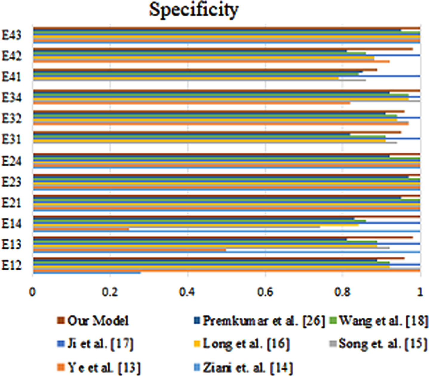
Specificity of the proposed method with existing methods.

5 Conclusion

This study introduces a novel fault diagnosis model for semiconductor manufacturing, leveraging generative adversarial networks (GANs). Addressing the challenge of accurate fault identification in complex processes, the manuscript details our approach, experimental setup, and comparison with existing models. Our methodology includes data extraction, a paired GAN-based generator model for predicting unknown target data, and a deep convolutional neural network implementation. Experiments span 12 shift tasks, assessing the model’s performance across various scenarios. Results reveal the proposed model’s superiority in accuracy, specificity, and sensitivity compared to six existing models. This model’s robustness in predicting normal and faulty portions underscores its reliability. Our contribution lies in presenting an efficient GAN-based approach for fault diagnosis, with promising implications for improving semiconductor manufacturing efficiency, quality, and process control. Future research will fine-tune the model for real-time applicability and potential expansion to other manufacturing sectors.

References

Zhang

, Gao

, Li

and Feng

, Fault Detection Strategy Based on Weighted Distance of k Nearest Neighbors for Semiconductor Manufacturing Processes, IEEE Transactions on Semiconductor Manufacturing 32(1) (2019), 75–81 10.1109/TSM.2018.2857818.

Jang

, Min

B.W.

and Kim

C.O.

, Denoised Residual Trace Analysis for Monitoring Semiconductor Process Faults, IEEE Transactions on Semiconductor Manufacturing 32(3) (2019), 293–301 10.1109/TSM.2019.2916374.

Huangang Wang , Ma Yao , Fault detection of batch processes based on multivariate functional kernel principal component analysis, Chemometrics and Intelligent Laboratory Systems 149(Part A) (2015), 78–89, ISSN 0169-7439.https://doi.org/10.1016/j.chemolab.2015.09.018.

N.P and S.P, Human emotions detection using kernel nonlinear collaborative discriminant regression classifier: Human emotions detection using KNCDRC, in 2021 2nd International Conference on Smart Electronics and Communication (ICOSEC), 2021, pp. 1807–1812. doi: 10.1109/ICOSEC51865.2021.9591878.

Kang

, Cho

, Anand

and Rim

, Using Wafer Map Features to Better Predict Die-Level Failures in Final Test, in IEEE Transactions on Semiconductor Manufacturing 28(3) (2015), 431–437 10.1109/TSM.2015.2443864.

Kang

, Joint modeling of classification and regression for improving faulty wafer detection in semiconductor manufacturing, Journal of Intelligent Manufacturing 31 (2020), 319–326. https://doi.org/10.1007/s10845-018-1447-2.

Fan

S.-K.S.

, Hsu

C.-Y.

, Tsai

D.-M.

, He

and Cheng

C.-C.

, Data-Driven Approach for Fault Detection and Diagnostic in Semiconductor Manufacturing, in, IEEE Transactions on Automation Science and Engineering 17(4) (2020), 1925–1936 10.1109/TASE.2020.2983061.

J.M.

, Hong

S.R.

, Choi

J.Y.

, et al. Wafer-to-wafer process fault detection using data stream mining techniques, International Journal of Precision Engineering and Manufacturing 14 (2013), 103–113. https://doi.org/10.1007/s12541-690013-0015-0.

and Zhao

, Online Fault Diagnosis for Industrial Processes With Bayesian Network-Based Probabilistic Ensemble Learning Strategy, in IEEE Transactions on Automation Science and Engineering 16(4) (2019), 1922–1932 doi: 10.1109/TASE.2019.2915286.

10.

Alankrita Aggarwal , Mamta Mittal , Gopi Battineni , Generative adversarial network: An overview of theory and applications, International Journal of Information Management Data Insights 1(1) (2021), 100004, ISSN 2667-0968.https://doi.org/10.1016/j.jjimei.2020.100004.

11.

Lee

K.B.

, Cheon

and Kim

C.O.

, A Convolutional Neural Network for Fault Classification and Diagnosis in Semiconductor Manufacturing Processes, in, IEEE Transactions on Semiconductor Manufacturing 30(2) (2017), 135–142 10.1109/TSM.2017.2676245.

12.

Liu

, Yan

, Zhang

C.-A.

and Liu

, An Ensemble Convolutional Neural Networks for Bearing Fault Diagnosis Using Multi-Sensor Data, Sensors 19 (2019), 5300https://doi.org/10.3390/s19235300.

13.

Wise

B.M.

, Gallagher

N.B.

, Butler

S.W.

, White

D.D.

and Barna

G.G.

, A comparison of principal component analysis, multiway principal component analysis, trilinear decomposition and parallel factor analysis for fault detection in a semiconductor etch process, Journal of Chemometrics 13 (1999).

14.

Ziani

, Felkaoui

and Zegadi

, Bearing fault diagnosis using multiclass support vector machines with binary particle swarm optimization and regularized Fisher’s criterion, Journal of Intelligent Manufacturing 28 (2017), 405–417. https://doi.org/10.1007/s10845-014-0987-3.

15.

Song

, Liu

, Li

Based on End-to-End Object Detection Algorithm with Transformers for Detecting Wafer Maps, in 2022 International Conference on Computer Network, Electronic and Automation (ICCNEA), Xi’an, China, 2022, pp. 297–302. doi: 10.1109/ICCNEA57056.2022.00072.

16.

Long

, Wang

, Ding

, Sun

, Yu

P.S.

Transfer Feature Learning with Joint Distribution Adaptation, in 2013 IEEE International Conference on Computer Vision, 2013, pp. 2200–2207. doi: 10.1109/ICCV.2013.274.

17.

, Lee

J.-H.

Using GAN to Improve CNN Performance of Wafer Map Defect Type Classification: Yield Enhancement, in 2020 31st Annual SEMI Advanced Semiconductor Manufacturing Conference (ASMC), Saratoga Springs, NY, USA, 2020, pp. 1–6. doi: 10.1109/ASMC49169.2020.9185193.

18.

Wang

, Chen

, Hao

, Feng

, Shen

Balanced Distribution Adaptation for Transfer Learning, in 2017 IEEE International Conference on Data Mining (ICDM), 2017, pp. 1129–1134. doi: 10.1109/ICDM.2017.150.

19.

Ghanem

W.A.H.M.

, et al. Cyber Intrusion Detection System Based on a Multiobjective Binary Bat Algorithm for Feature Selection and Enhanced Bat Algorithm for Parameter Optimization in Neural Networks, in IEEE Access 10 (2022), 76318–76339 doi: 10.1109/ACCESS.2022.3192472.

20.

Palanichamy Naveen , Pothiraj Sivakumar , A deep convolution neural network for facial expression recognition, Journal of Current Science and Technology 11(3) (2021), 402–410. doi: 10.14456/jcst.2021.40.

21.

Zhang

, Wang

, Pan

and Pan

, Imbalanced Fault Diagnosis of Rolling Bearing Using Enhanced Generative Adversarial Networks, in IEEE Access 8 (2020), 185950–185963. doi: 10.1109/ACCESS.2020.3030058.

22.

Lee

J.H.

and Lee

J.M.

, Progress and challenges in control of chemical process, Annual Review of Chemical and Biomolecular Engineering 5(1) (2014), 383–404.

23.

Q.P.

and Wang

, Large-Scale Semiconductor Process Fault Detection Using a Fast Pattern Recognition-Based Method, in IEEE Transactions on Semiconductor Manufacturing 23(2) (2010), 194–200 doi: 10.1109/TSM.2010.2041289.

24.

Yunusa-Kaltungo

and Sinha

J.K.

, Sensitivity analysis of higher order coherent spectra in machine faults diagnosis, Structural Health Monitoring 15(5) (2016), 555–567. https://doi.org/10.1177/1475921716651394.

25.

Kim

, Cho

, Lee

and Cho

, Fault Detection and Diagnosis Using Self-Attentive Convolutional Neural Networks for Variable-Length Sensor Data in Semiconductor Manufacturing, in IEEE Transactions on Semiconductor Manufacturing 32(3) (2019), 302–309 doi: 10.1109/TSM.2019.2917521.

26.

Premkumar

, Ashokkumar

S.R.

, Mohanbabu

, Jeevanantham

and Jayakumar

, Security behavior analysis in web of things smart environments using deep belief networks, International Journal of Intelligent Networks 3 (2022), 181–187, ISSN 2666-6030.https://doi.org/10.1016/j.ijin.2022.10.003.

27.

Suthar

, Vakharia

, Patel

V.K.

and Shah

, Detection of Compound Faults in Ball Bearings Using Multiscale-SinGAN, Heat Transfer Search Optimization, and Extreme Learning Machine, Machines 11(1) (2023), 29. https://doi.org/10.3390/machines11010029.

28.

Han

, Hao

, Cheng

and Xu

, GAN-SAE based fault diagnosis method for electrically driven feed pumps, PLOS ONE 15(10) (2020), e0239070.https://doi.org/10.1371/journal.pone.0239070.

29.

Shah

, Borade

, Sanghavi

, Purohit

, Wankhede

and Vakharia

, Enhancing Tool Wear Prediction Accuracy Using Walsh–Hadamard Transform, DCGAN and Dragonfly Algorithm-Based Feature Selection, Sensors 23(8) (2023), 3833.https://doi.org/10.3390/s23083833.