
Abstract
During the period of 2019–20, forecasting was of utmost priority for health care planning and to combat COVID-19 pandemic. Almost everyone’s life has been greatly impacted by COVID-19. Understanding how the disease spreads is crucial to know how the disease behaves dynamically. The aim of the research is to construct an SEI Q1Q2 R model for COVID-19 with fuzzy parameters. The fuzzy parameters are the transmission rate, the infection rate, the recovery rate and the death rate. We compute the basic reproduction number, using next-generation matrix method, which will be used further to study the model’s prediction. The COVID-free and endemic equilibrium points attain local and global stability when R0 < 1. A sensitivity analysis of the reproduction number against its internal parameter has been done. The results of this model showed that intervention measures. The numerical simulation along with graphical representations at COVID-free and endemic points are shown. The SEIQ1Q2R model is a successful model to analyse the spreading and controlling the epidemics like COVID-19.
Introduction
The universe was brought to its knees by the COVID-19 illness epidemic during its inversion. A coronavirus is a CORONAVIRIDAE member that affects several vertebrates by causing gastrointestinal or respiratory illness [1]. When the sickness began to spread globally in early 2020 after its origin in Wuhan, China, in December 2019 [2], the world went through difficult times. The disease was initially discovered in Wuhan, the capital of Hubei, China, in December 2019. Since then it has spread around the world, leading to the 2020 pandemic breakout [3]. Due to the thousands of confirmed illnesses and thousands of deaths worldwide, the COVID-19 pandemic was regarded as the greatest global threat. Several approaches to assess and predict the pandemic’s evolution have been made as a result of the interest shown by experts from various fields in the worldwide challenge of the outbreak [4, 5]. In a short period of time, the sickness sickened millions of people globally and claimed 100,000 lives, causing unrest in every country. The World Health Organization (WHO) established disease-fighting tactics at the time to battle the pandemic and preserve lives. The strategic tactics included quarantine, physical and social seclusion, mask usage, border closures, and economic lock-downs. The actions taken had a social and economic impact on the planet. The most effective method of combating COVID-19 is immunization, which also helps to restore lost economic activity [6–8]. Scientists have developed a variety of vaccinations to battle the illness, and the WHO has approved them [9]. The study conducted by [10] examined vaccination in age group allocation techniques with their SEIR model in India and came out with the results revealing that the elderly generation aged more than 60 years, which was the most affected group by COVID-19 disease, was the group considered for vaccination. Moreover, [11] discussed a model with an age structure and time-varying contact rates.
As shown in the study [12], mathematical models are highly important tools used to assess the likelihood and severity of the disease and assist in determining the intervention measures to be implemented to battle and control the disease intensity. The article [13] discussed the future situation, after the calculation of reproduction number. The results of the manuscript [14], were used as an early prevention of the spread of COVID-19 in Indonesia. Many mathematical models have been developed since the COVID-19 outbreak first started. A compartmental model of the progression of chronic diseases, human epidemiological state, and intervention strategies was put forth by Tang et al. [15] and was deterministic. The manuscript [36] Huanlai Xing et.al proposed a robust semisupervised model with self-distillation that simplified existing semisupervised learning techniques for extracting high level semantic information, which is also helpful for capturing low level semantic information. A novel robust temporal feature network which was responsible for extracting local features was proposed [37]. The authors discovered that there can be up to 6.47 reproductive controls, and that engagement strategies like streamlined traceability combined with isolation and quarantine may successfully reduce the number of reproductive controls and transmission risk. Iman et al. [16] performed calculational modelling of the potential epidemic tracks with a focus on human-to-human transmissions to figure out the extent of the illness outbreak in Wuhan. According to its findings, more than 60% of the transmission must be effectively regulated in order to control the disease. Authors like Ahmaed, Parvaiz, Ihtisham, Fatma and Anne investigated the novel corona virus using various methods [38–40, 48]. In the manuscript [41], authors have suggested a new model that represents the interplay of two diseases (corona and bacterial pneumonia) by taking into account the two different ways that pneumonia can be acquired: in the community and in a hospital. They’ve demonstrated through numerical simulations that both diseases can endure if COVID’s basic reproduction number is higher than one. The model depicted MERS-CoV transmission between individuals and reservoirs like camels. The model was created with optimal control in view to reduce the number of infected people while keeping intervention costs low [44]. Using Caputo-Fabrizio advention reaction diffusion equation Hardik analyzed the effect of disturbance in intracellular calcium dynamic on fibroplast cell [45]. The majority of the models showed how important a direct human-to-human transmission mechanism was in the outbreak, which was supported by the observation that many of the infected people in the Wuhan region do not interact with one another and that the number of infections has been rising quickly and spreading to other Chinese provinces, affecting more than 20 people [17]. Hardik along with various co-authors have investigated several models for the spread of COVID-19 using Caputo fractional derivative, Adam-type predictor corrector, ABC derivative [42, 47]. To obtain an approximate solution, the Laplace. The suitable strategies for quarantine during the COVID-19 pandemic in a specific age group were first presented by Gondim and Machado [18]. Wang et. al used the mathematical model to deduce the earliest start date of COVID-19 infection in Wuhan [19]. The SEIR model was updated by Youssef et al. [20] and applied to the actual data of COVID-19 spreading in Saudi Arabia. Feng and Thieme [21, 22] evaluated the model dynamics of SEIQR (Susceptible-Exposed-Infected-Quarantined-Recovered) models with arbitrarily spaced periods of sickness, together with quarantine, and a general occurrence stated that all affected patients passed through the quarantine stage. A pandemic influenza SEIQR model for obtaining the numerical values of the model’s parameters was proposed by Jumpen et al. [23] who also examined the model’s characteristics. For paediatric illnesses, Gerberry and Milner [24] employed the SEIQR model. The authors of the articles [13, 18–22] evaluated the mathematical model with different compartments. They have computed basic reproduction number, analysed stability of the disease and some of them concluded with control strategies. This provided the motivation to add fuzzy analysis in this manuscript.
Deterministic models with fixed model parameters have been adopted by the majority of researchers. In general, they made the assumptions that each person could spread the disease and recover from it at a constant rate. The assumptions, however, be contrary to the actual epidemic. As a result, in the current study, we have taken a few parameters into account as fuzzy parameters. So, the purpose of this research is to develop a new COVID-19 dynamical model using mathematical analysis that is more applicable to scenarios in any country. Our model demonstrates how the corona virus spreads via interaction with an infected person who is carrying a variety of virus loads and depicts the transmission of the disease at both endemic and COVID-free equilibrium points. The outbreak is brought on by the new infections. In view of this, future predictions of the spread of any pandemic may be enhanced as a result of our research.
Transmission of COVID-19
The WHO Country Office in China initially received a report of a pneumonitis of unknown origin on December 31, 2019 [25]. Animal-to-human transmission was assumed to be the primary route because the first instances of the CoVID-19 disease were directly connected to exposure to the Huanan Seafood Wholesale Market in Wuhan, Republic of China. However, later occurrences were not connected to this exposure mechanism. Therefore, it was determined that the virus could potentially transfer from person to person and that symptomatic individuals constitute the main channel for COVID-19 transmission. Transmission prior to the onset of symptoms appears to be uncommon, although it cannot be ruled out. Furthermore, there are theories that those who are asymptomatic could spread the infection. According to the research, isolation is the most effective method for controlling this outbreak [26]. The longest time from infection to symptoms was 12.5 days (95% confidence interval, 9.2 to 18), according to data from the first cases in Wuhan and investigations by the Chinese Centre for Disease Control and Prevention (CDC) and local CDCs [27]. The incubation period could typically be between 3 and 7 days and up to 2 weeks. Additionally, this information demonstrated that this unusual pandemic doubled roughly every seven days, although the fundamental rate of production (R0) is 2.2. In other words, each patient typically spreads the sickness to an additional 2.2 others. The reproduction number of the SARS-CoV epidemic in 2002–2003 was estimated to be around 3 [28]. According to a study, humans can develop coronavirus by inhaling it or by touching contaminated materials. Researchers found that the virus can be detected in aerosols for up to three hours, on copper for up to four hours, on cardboard for up to 24 hours, and on plastic and stainless steel for up to two to three days [29]. According to a recent study led by researchers at the Johns Hopkins Bloomberg School of Public Health [30], an analysis of publicly available data on infections from the new coronavirus, SARS-CoV-2, which causes the respiratory illness, COVID-19, produced an estimate of 5.1 days for the median disease incubation period. According to the data, around 97.5 percent of those who experience SARS-CoV-2 infection symptoms do so within 11.5 days after exposure. For every 10,000 people isolated for 14 days, Lauer et al. estimated that only approximately 101 would exhibit symptoms after being let out [30].
Basic terminologies
Assumptions
The population is considered as a heterogenous population. Birth rates are assumed to be a susceptible population. The following takes place at a constant rate:
The birth rate and natural deaths. Death due to COVID-19 of the medically quarantined population. Exposed population becoming susceptible under home quarantine. Contact rate The rate of susceptible population who were in their home becoming susceptible whose reports are negative. Rate of infected population who undergo medical quarantine Susceptible population under home quarantine Medical quarantine population of confirmed cases.
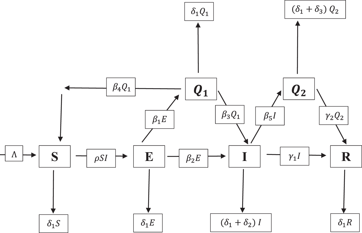
Fuzzy mathematical model
The following is the system of fuzzy mathematical model for COVID-19, followed by overview of the parameters in Table 1.
Overview of the parameters
Overview of the parameters
Fuzzy analysis
β3 = β3 (ϑ) be the chance of transmission rate from susceptible people to the infected. The virus load affects how quickly diseases spread. The following equation shows the fuzzy membership function for the transmission parameter.
When the virus load is very low (ϑ min ), as shown by the equation, there is almost little chance of virus transmission. For transmission to take place, there must be a specific quantity of virus present (ϑ M ). Each disease’s virus burden is always limited by ϑ max .
The Fig. 1 shows the membership function of β3 (ϑ).
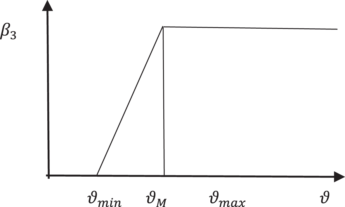
Membership function of β3.
Let β2 = β2 (ϑ) be the rate at which the exposed population becomes infected. The Figs. 2 and 3 are the representation of membership function of β2 (ϑ) and γ1 (ϑ).
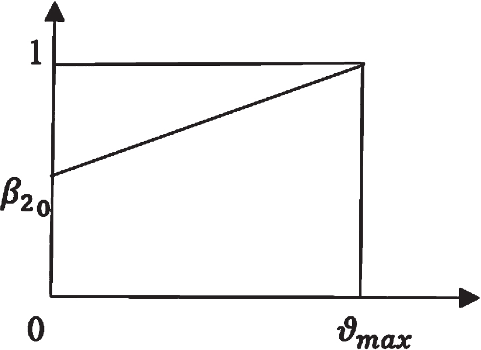
Membership function of β2.
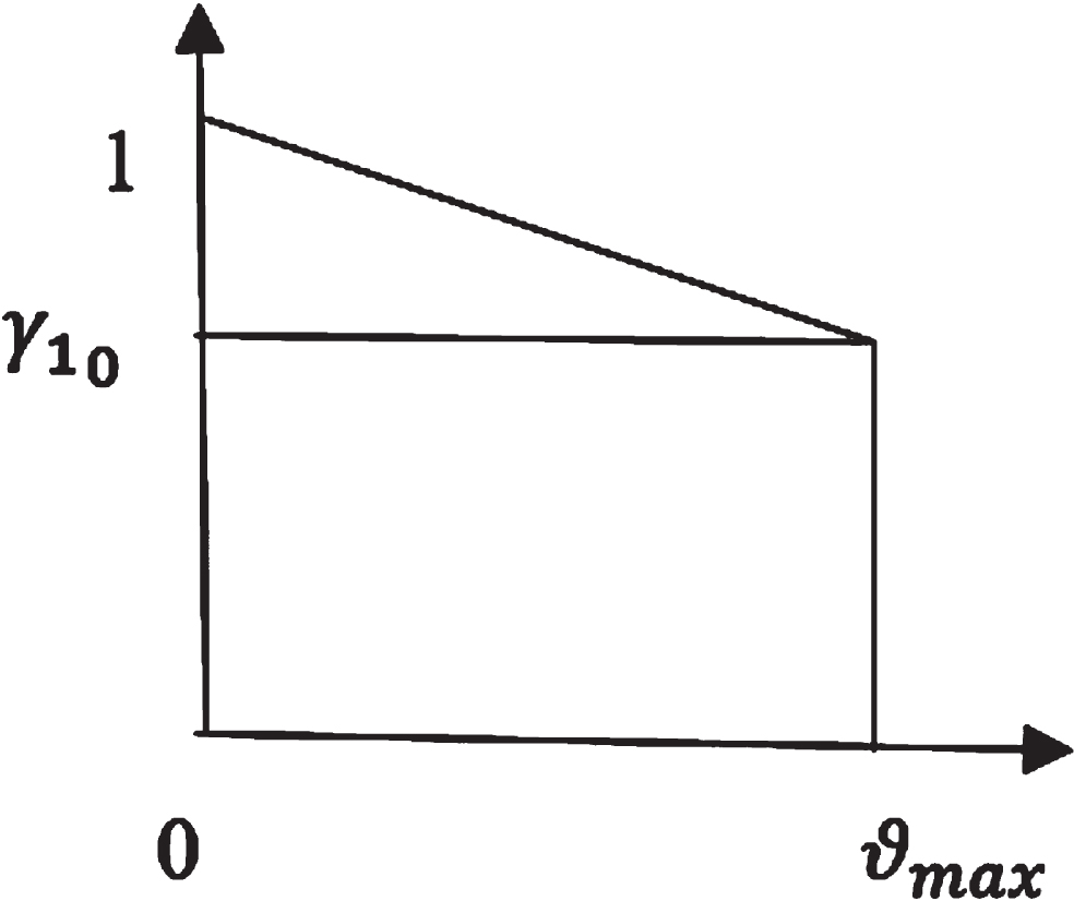
Membership function of γ1.
Let γ1 = γ1 (ϑ) be the recovery rate from infectious population.
Let γ2 = γ2 (ϑ) be the recovery rate from medical quarantined population.
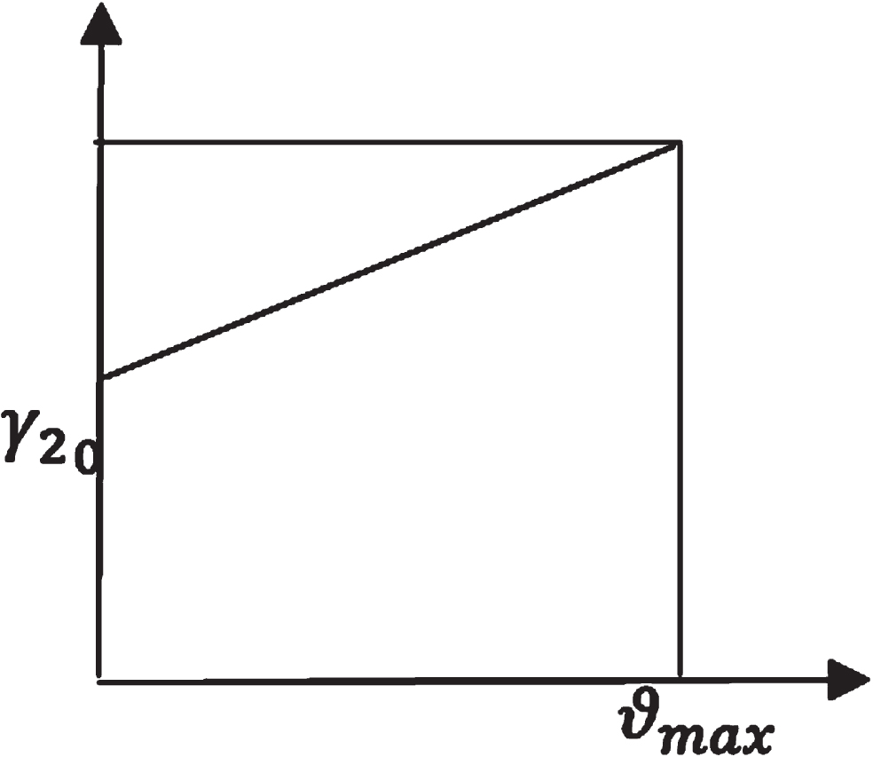
Membership function of γ2.
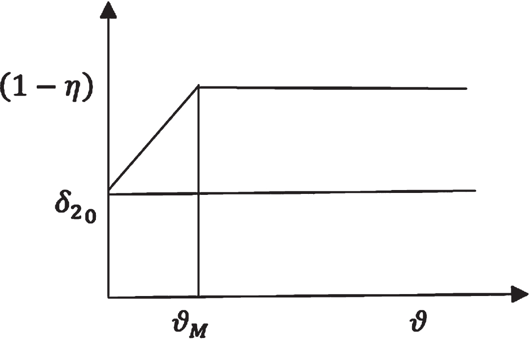
Membership function of δ2.
δ2 = δ2 (ϑ) Be the rate of death due to COVID-19
COVID-free equilibrium
Endemic equilibrium
Basic reproduction number (BRN)
The basic reproduction is defined as the average numbe secondary infections when one infectious agent is introduced into a population that is completely susceptible. It is calculated using the next generation matrix method.
Asymptotic stability analysis
The characteristic equation is λ3 + a1
λ2 + a2
λ + a3 = 0
According to Routh-Hurwitz criteria a1 > 0, a2 > 0, a3 > 0, a1a2 > a3 (Refer Appendix: 1). Thus the system is locally asymptotically stable.
Global stability
Consider,
Let, C1 = δ1 (β3 + β4 + δ1) (β5 + γ1 + δ1 + δ2),
C2 = ρ ∧ (β1 β3 + β2 β3 + β2 β4 + β2δ1)/β1,
C3 = - δ1 (β1 + β2 + δ1) (β3 + β4 + δ1) (β5 + γ1 + δ1 + δ2)/β2
≤δ1 (β1 + β2 + δ1) (β3 + β4 + δ1) (β5 + γ1 + δ1 + δ2) [R0 - 1]
Consider,
Let C1 = (β1 β3 + β2 β3 + β2 β4 + β2δ1) - [δ1 (β1 + β2 + δ1) (β3 + β4 + δ1) (β5 + γ1 + δ1 + δ2)],
C3 = (β1 + β2 + δ1) (β3 + β4 + δ1)
≤ (β1 + β2 + δ1) (β3 + β4 + δ1) (β5 + γ1 + δ1 + δ2) [R0 - 1].
Consider,
Let C2 = δ1 (β1 + β2 + δ1) (β5 + γ1 + δ1 + δ2),
C3 = {ρ ∧ (β1 β3 + β2 β3 + β2 β4 + β2δ1) – [δ1 (β1 + β2 + δ1) (β5 + γ1 + δ1 + δ2) (β3 + β4 + δ1)}/β3
≤δ1 (β1 + β2 + δ1) (β5 + γ1 + δ1 + δ2) (β3 + β4 + δ1) [R0 - 1].
Hence by LaSalle’s invariance principle [34], hence the system is globally stable at COVID-free equilibrium.
Fuzzy basic reproduction number (FBRN)
The basic reproduction number is R0
(γ10 R0 (ϑ)) is
Where FEV (γ10 R0 (ϑ)) = sup {inf (α, k (α))}, 0≤ α ≤ 1,
k (α) = , is a fuzzy measure [33]. To get FEV (γ10 R0 (ϑ)) we, define fuzzy measure μ,
μ (X) = supΓ (ϑ), ∀σ ∈X, X ⊂ R, which is a possibility measure.
From FEV (γ10 R0 (ϑ)), it is clear that R0 (ϑ) is not decreasing with, where the set, X = [
Thus, k (α) = μ [ϑ′, ϑ max ] = sup Γ (ϑ) with ϑ′ ≤ ϑ ≤ ϑ max , here k (0) = 1 and k (1) = Γ (ϑ max ).
The virus loads which are linguistic variable can be classified as low virus load (ϑ min ), medium virus load (ϑ) and strong virus load (ϑ max ).
Case 1: Low virus load
(i.e) when
FEV (γ10 R0 (ϑ)) = 0 <
As a result, we may say that the disease will vanish.
Case 2: Medium virus load
(i.e) when
Therefore,
So, if δ > 0, k(α) is continuous and decreasing function with k(0) = 1 and k(1) = 0. Hence, FEV (γ10 R0 (ϑ)) is the fixed point of k and
As the function R0 (ϑ) is increasing and continuous function then by the intermediate value theorem there exists ϑ with
Case 3: Strong virus load
(i.e)
Similar to case 2, we have
Thus,
Numerical simulation
Bhilwara is a district in Rajasthan, India which is referred to as the nation’s textile capital. The size of Bhilwara district is about 10,455 square kilometres and the population density of 230 persons per square kilometre. Bhilwara is one of the first Indian towns to become hub for positive infection of corona virus. During the initial stages of the COVID-19 outbreak, the Bhilwara dtrict was one of India’s most severely impacted areas. By March 22, 2020, the Health Department and the district administration in Bhilwara had organised over 850 teams, conducted house-to-house surveys at 56,025 homes and interviewed 280937 people, all within three days of the first positive case. Patients who were tested positive underwent intense contact tracing, and the Health Department created detailed documentation of every person they have come into touch with since being sick. Essentials were arranged by administrators. The majority of the infected cases were found and quarantined as the number of tests grew. The district was divided off by the local government, which also established a containment zone of 1km from the epicentre and a 3km long buffer zone. Continuous screening was done along with cluster mapping.
The initial conditions are S (0)=0.69, E (0)=0.27, Q1 (0)=0, I (0)=0.03, Q2 (0)=0.01, R (0)=0 [35].
Parametric values for COVID-free equilibrium
Parametric values for COVID-free equilibrium
In Fig. 6a, represents the susceptible population which increases with respect to time, b represents the number of exposed population, where the curve decreases which indicates that the number of individuals from exposed compartment are moving to infected compartment, c represents the number of infected population due to disease, d represents the number of susctible population under home quarantine, e represents the number of population under medical quarantine who were tested positive for the disease and f represents the number of recovered population.
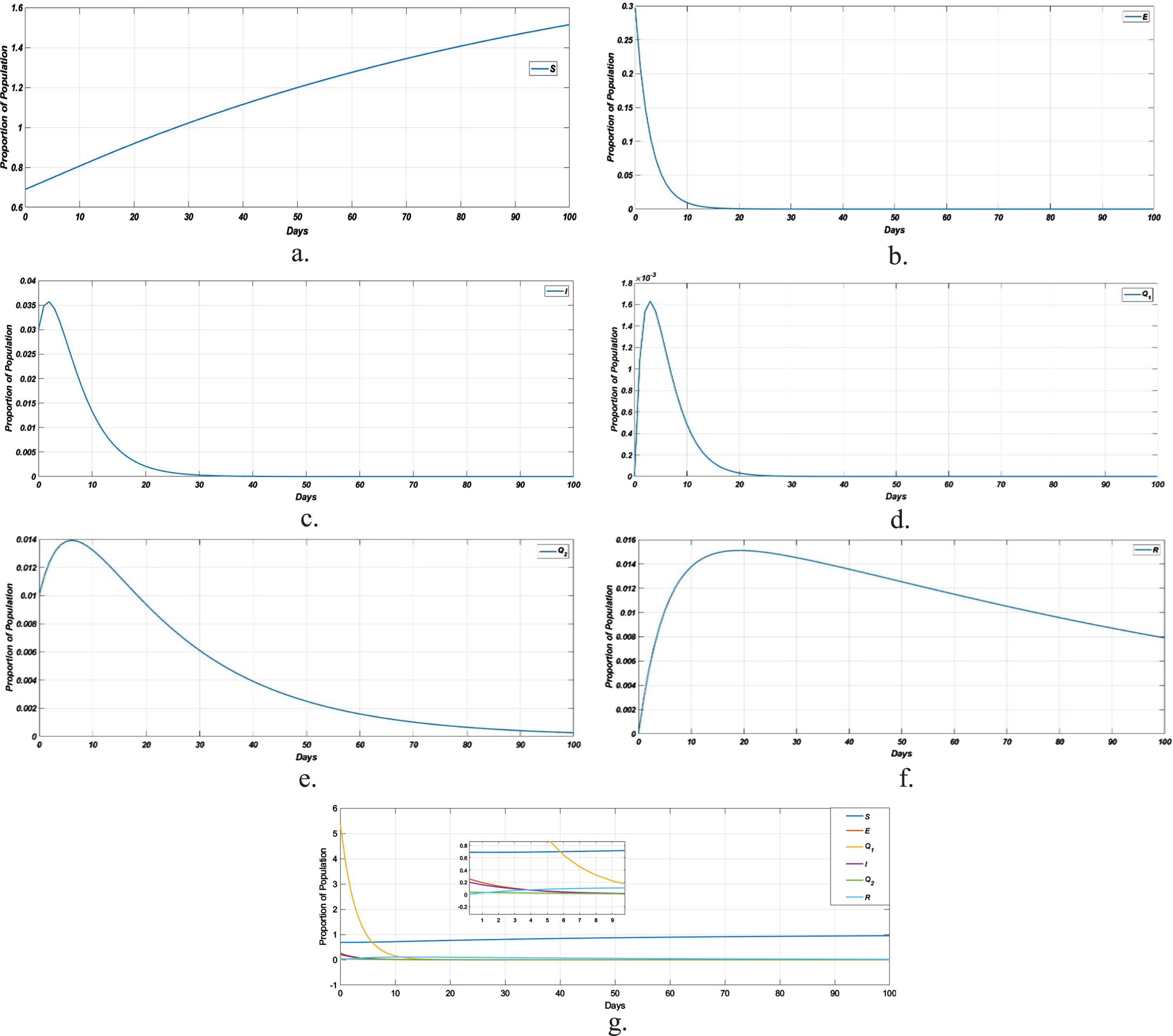
Solution of Homotopy pertubation method at t = 0 to 100. a. Susceptible population; b. Exposed population; c. Infected population; d. Susceptible population under home quarantine; e. Medical quarantined population of confirmed cases; f. Recovered population; g. dynamical behavior of the model at COVID-free equilibrium.
Parametric values for endemic point
In Fig. 7a, represents the susceptible population at endemic equilibrium point; b, represents the number of exposed population at endemic equilibrium point; c, represents the number of infected population at endemic equilibrium point; d, represents the number of susceptible population under home quarantine at endemic equilibrium point; e, represents the number of population under medical quarantine of confirmed cases at endemic equilibrium point and f represents the number of recovered population at endemic equilibrium point.
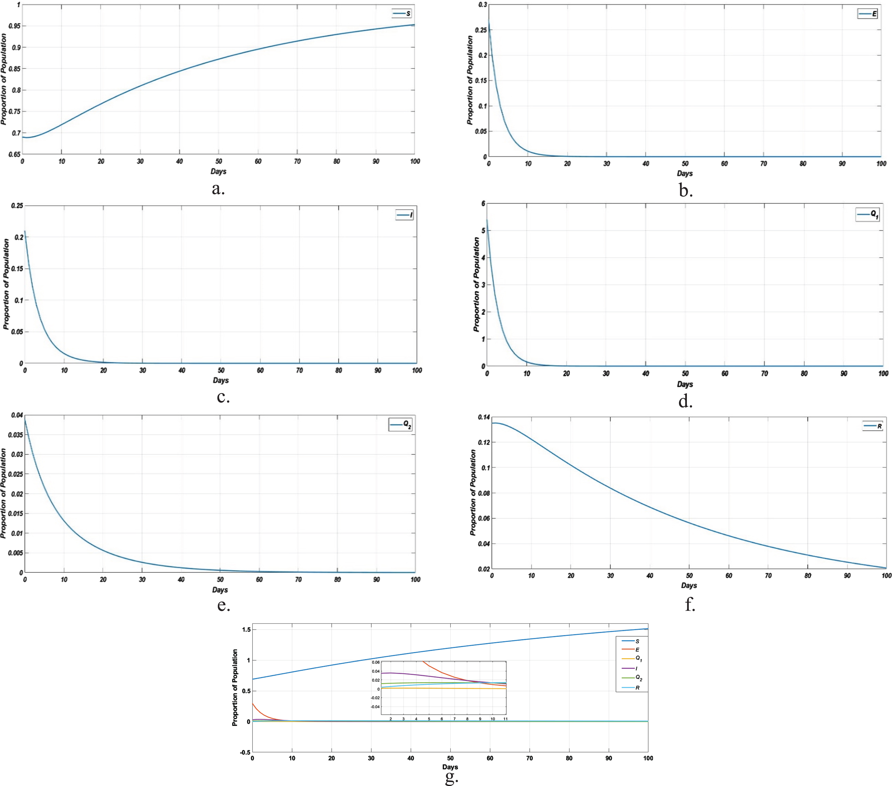
Solution of Homotopy pertubation method at t = 0 to 100. a. Susceptible population; b. Exposed population; c. Infected population; d. Susceptible population under home quarantine; e. Medical quarantined population of confirmed cases; f. Recovered population; g. dynamical behavior of the model at endemic equilibrium.
Our main concern is to know about the pandemic’s potential to infect a population. Sensitivity analysis is used to examine the elements that contribute to the spread and persistence of this disease in the community. We focus on the variables that cause a greater variance in the value of the basic reproduction number.
The sensitivity indices can be defined as follows [31]
The sensitivity index of R0 can be obtained from the above definition. The Table 1 below shows the sensitive indices of each parameter. The reproduction rate will rise with an increase in the sensitivity index number, and the reproduction rate will fall with a decrease in value, which in turn results in a reduction in the spread of disease. The Table 4 shows the sensitive index values for the parametric values in Table 2 and Fig. 8 shows its graphical representation.
Sensitive index for COVID-free equilibrium
Sensitive index for COVID-free equilibrium
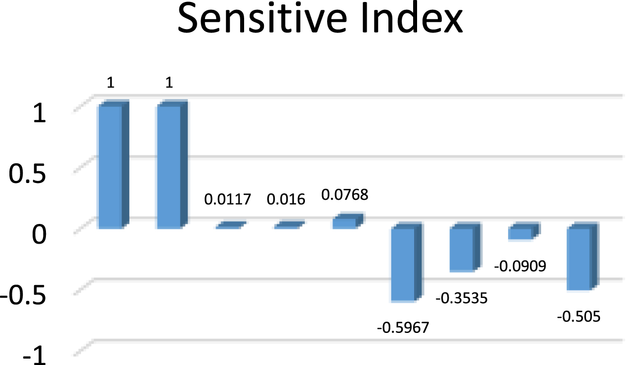
Sensitive index for COVID-free equilibrium.
The Table 5 shows the sensitive index values for the parametric values in Table 3 and the Fig. 9 shows it’s the graphical representation.
Sensitive index for endemic equilibrium
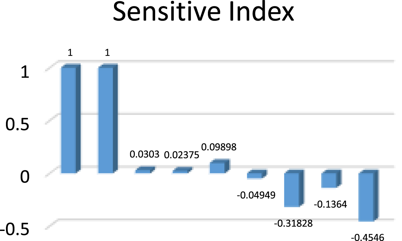
Sensitive Index for endemic equilibrium.
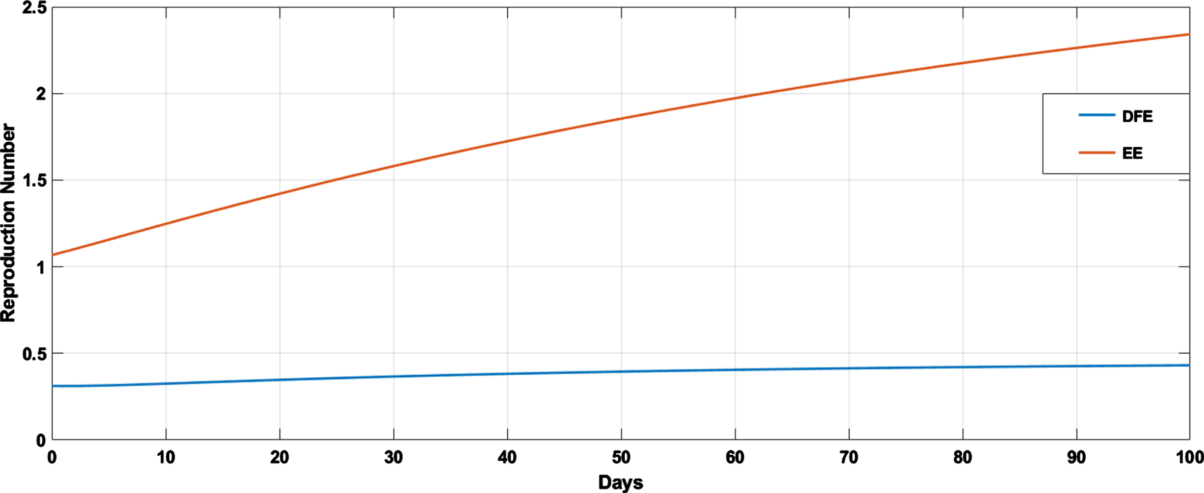
Reproduction number at COVID-free equilibrium.
The only measures to prevent further spread were the time-tested practices of quarantine, case isolation, travel restrictions, and barrier precautions. The first line of protection against new deadly diseases will undoubtedly be such control measures, which have been used for ages. Without the use of models, the qualitative effect of control measures is known: they tend to reduce transmission. Models, on the other hand, offer a strict framework for analysis that gives a sophisticated, quantitative knowledge of the influence of control measures. Instead of being dependent on control and epidemiologic characteristics in a straightforward additive manner, the effectiveness of numerous control measures may depend on them in a complex, nonlinear way. The efficacy of numerous control measures may be complex, nonlinear, and dependent on control and epidemiologic characteristics rather than simply additive. When control measures are too expensive, difficult, or burdensome, detailed modelling can assist in determing whether and when partial relaxation of particular control measures is beneficial.
Conclusion
An SEQ1 IQ2 R model has been developed for which local and global asymptotic stability is well established. The estimation of possible extent of the transmission is given by the basic reproduction number. There is negligible disease transmission when the system’s basic reproduction number is less than one, and when it is larger than one, the disease begins to spread more quickly. According to reality, not all sick people spread the disease in the same way, and each person has a unique level of disease infectivity that varies depending on their virus loads. The virus load classification aids in understanding of the fuzzy reproduction rate. The sensitive index provides scientists and the government with a clear picture that they can use to formulate policies to stop the disease’s spread and to take preventative action against and manage future pandemics caused by other new viruses. To establish the analytical results, numerical simulations using actual parric values are carried out.
Footnotes
Appendix 1
We show that a1 > 0, a2 > 0, a3 > 0, a1a2 > a3
a1= [0.3 + 0.05+(3 * 0.01)+0.3 + 0.02 + 0.07 + 0.1+ 0.018]
a1= 0.888
a2= [(0.3 + 0.05 + 0.01) (0.3 + 0.02 + 0.01)]+[(0.3 + 0.05 + 0.01) (0.07 + 0.1 + 0.01 + 0. 018)]+[(0.07 + 0.1 + 0.01 + 0.018) (0.3 + 0.02 + 0.01)]
a2= 0.25542
a3= [(0.3 + 0.05 + 0.01) (0.3 + 0.02 + 0.01)×(0.07 + 0.1 + 0.01 + 0.018)] –(0.1*0.3*0.3)
a3= 0.0145224.
And a1*a2= 0. 888 * 0.25542 = 0.22681296> a3 (= 0.0145224)