Emotion recognition from speech signals using digital features optimization by diversity measure fusion

Abstract

Emotion recognition from speech signals serves a crucial role in human-computer interaction and behavioral studies. The task, however, presents significant challenges due to the high dimensionality and noisy nature of speech data. This article presents a comprehensive study and analysis of a novel approach, “Digital Features Optimization by Diversity Measure Fusion (DFOFDM)”, aimed at addressing these challenges. The paper begins by elucidating the necessity for improved emotion recognition methods, followed by a detailed introduction to DFOFDM. This approach employs acoustic and spectral features from speech signals, coupled with an optimized feature selection process using a fusion of diversity measures. The study’s central method involves a Cuckoo Search-based classification strategy, which is tailored for this multi-label problem. The performance of the proposed DFOFDM approach is evaluated extensively. Emotion labels such as ‘Angry’, ‘Happy’, and ‘Neutral’ showed a precision rate over 92%, while other emotions fell within the range of 87% to 90%. Similar performance was observed in terms of recall, with most emotions falling within the 90% to 95% range. The F-Score, another crucial metric, also reflected comparable statistics for each label. Notably, the DFOFDM model showed resilience to label imbalances and noise in speech data, crucial for real-world applications. When compared with a contemporary model, “Transfer Subspace Learning by Least Square Loss (TSLSL)”, DFOFDM displayed superior results across various evaluation metrics, indicating a promising improvement in the field of speech emotion recognition. In terms of computational complexity, DFOFDM demonstrated effective scalability, providing a feasible solution for large-scale applications. Despite its effectiveness, the study acknowledges the potential limitations of the DFOFDM, which might influence its performance on certain types of real-world data. The findings underline the potential of DFOFDM in advancing emotion recognition techniques, indicating the necessity for further research.

1 Introduction

In the realm of “artificial intelligence (AI)” as well as“machine learning (ML)”, one of the areas that has sparked considerable interest and research is the recognition of human emotions from speech signals. This complex task is critical for a myriad of applications, encompassing the realms of interactive voice response systems, mental health diagnostics, virtual personal assistants, human-robot interaction, and more. It is fair to believe that speech emotion detection could be utilized to extract resourceful semantics from speech [1]. As a result, the performance of voice recognition approaches is improved. Recognizing emotion is especially advantageous for pre-requisite natural machine communication applications such as computer tutorials and online videos, as systems’ responses to the user are contingent on the emotion recognized [2, 3]. Additionally, it is advantageous for the in-car board technique, in which driver mental state data may be provided to the system for the purpose of commencing their safety [4]. Additionally, it may be beneficial in computer aided translating processes in which the speaker’s state of emotion plays a significant role in the interaction between the parties [5].The use of voice emotion recognition in mobile communications and contact center applications is most interesting aspect [6, 7]. The primary goal of emotion recognition from speech signals is to alter the system’s reaction when it detects displeasure or impediment in the speaker’s speech.

Despite its significance, accurate and efficient emotion recognition from speech signals continues to pose notable challenges. These challenges primarily stem from the intricacy and variability of human emotions, the high-dimensionality of speech data, and the difficulty of pinpointing the most meaningful and informative features from this data. The very nature of speech signals, which encompass a vast array of acoustic, prosodic, and spectral features, adds another layer of complexity to the task.

Addressing these intricate challenges, we present, “Emotion Recognition from Speech Signals Using Digital Features Optimization by Diversity Measure Fusion.” This comprehensive research work brings to the forefront a robust and innovative technique “Digital Features Optimization by Diversity Measure Fusion (DFOFDM)”. Our proposed approach is specifically designed to handle the aforementioned challenges by optimizing the selection of features from speech signals, leading to a more accurate emotion recognition process. Additionally, a meta-heuristic search technique cuckoo search has been tailored to perform classification of the emotions to categorize speech signals according to their emotional content.The “Cuckoo Search (CS)” algorithm, a metaheuristic method inspired by nature, is used in this novel method to enhance the selection and classification of features in emotion identification. The CS algorithm mimics the parasitic behavior of cuckoos to effectively optimize the search for the best features and parameters.

DFOFDM harnesses the power of three robust statistical tests - the “Kolmogorov–Smirnov test”, “Mann–Whitney U Test”, and the “two-tailed t-test”. These tests, traditionally employed to examine the differences between two independent probability distributions, are ingeniously combined in our methodology to measure the diversity of features. By doing so, we ensure the extraction of diverse yet informative features, thereby bolstering the effectiveness of the overall emotion recognition system.

Moreover, the crux of our methodology lies in its ability to assess and optimize the features within a speech signal. We venture beyond the simplistic approach of identifying the features with the highest individual performance, towards an integrated feature optimization system that leverages diversity for superior performance. This makes it possible to examine the interrelationships as well as dependencies between the characteristics in greater detail, taking into consideration the possible cumulative impact they may have on the efficacy of the emotion identification process.

We carefully assess DFOFDM in the context that our study article. Our results highlight the better efficacy and efficiency of our suggested technique, displaying a significant increase in the tasks’ accuracy for emotion identification.

The practical implications of our study are far-reaching. By improving the precision and efficiency of emotion recognition from speech signals, we contribute to the development of more effective human-computer interaction systems. From voice-activated virtual assistants that can accurately discern the emotional context of user commands, to mental health applications that can track and assess emotional well-being based on vocal cues, the potential applications are extensive.

The rest of the manuscript organized as follows. Section 2 explores the contemporary literature on feature extraction and classification of speech emotion recognition. Section 3 and subsequent sections explores the methods and materials used in proposed feature engineering and classification of emotions for speech emotion recognition. Further, followed by experimental study as section 4. Section 5 explores conclusions of proposed model and corresponding findings that followed by references.

2 Related work

Features that are unnecessary or redundant are what feature selection algorithms are designed to get rid of. In contrast, doing an exhaustive search of entire subset space is intractable as well as NP-Hard [8, 9]. Genetic algorithms and Ant-Colony [10–12] have been used to solve this problem because they have a tendency to discover the best subsets when searching for the best features in a given space.Stochastic search techniques use “genetic algorithms (GA)” with natural selection [13]. GA might be single-objective or multi-objective. To find speech emotion identification components, A multi-objective evolutionary strategy with certain tweaks was proposed by Brester et al. [10]. Another evolutionary method found in recent works is particle swarm optimization, which uses a feature selection method based on biogeography. Artificial “BCO (bee colony optimization)” and “GB (gradient boosting)” were presented in a decision tree by Rao H et al. [14]. A recent application of NSGA II for feature selection was published by Kozodoi et al. [15]. The NSGA-II, used to evaluate products, is suggested to be revised by Li A-D et al. [12].

To address feature selection challenges in classification tasks, Pereira, a novel approach called “Binary Cuckoo Search (BCS)” proposed L. A. M., et al. [16]. The authors have shown that BCS is superior than “Particle Swarm Optimisation (PSO)” and “Genetic Algorithm (GA)”, two additional bio-inspired optimisation methods. However, the paper’s conclusions may be overly specific because it focuses solely on binary feature selection and evaluates its efficacy using the OPF classifier.

“Cuckoo Search (CS)” is a new method for solving global optimisation issues, and Deb, S.and Yang, X. S., [17] explore its inner workings. The authors provide an in-depth examination of the search processes used by the algorithm to prove its usefulness. Despite showing excellent performance in a variety of scenarios, the authors concede that the success of an algorithm is highly dependent on the nature of the problem being tackled.

Gunavathi, C. and Premalatha, K. [18] present a unique approach for feature selection for cancer classification by applying the CS optimised algorithm to microarray gene expression data. The authors demonstrate that, particularly in datasets including cancer gene expression, this method increases classification accuracy. Despite these positive results, more study is necessary owing to the method’s drawbacks, including a low possibility of properly identifying an outside egg as well as a small number of host nests.

For the purpose of recognising children’s emotions based on voice signals and face pictures, Albu, F., Hagiescu, D., et al. [19] investigate several neural network techniques. According to the study’s findings, children’s emotional states have a significant impact in improving learning outcomes using intelligent tutoring systems. Despite this important addition, the authors only classify emotion recognition into three categories— positive, negative, and neutral-suggesting there is need to broaden this study to cover a wider range of emotions.

An innovative method for learning from salient features for “speech emotion recognition (SER)” using “convolutional neural networks (CNN)” was developed by Dong, M., Mao, Q., et al. [20]. The paper’s primary contributions are the following: the introduction of feature learning to SER; the proposal of a novel objective function in “salient discriminative feature analysis (SDFA)” that promotes feature saliency, orthogonality, and discrimination; and the demonstration of the superiority of the learned features over established feature representations in recognizing emotions in complex scenes. Training occurs in two phases: first, “local invariant features (LIF)” are learned with a “sparse auto-encoder (SAE)”, and then, in a second phase, affect-salient features “(SDFA)” are learned. The suggested method might be used to automatically extract features and improve SER’s recognition accuracy and stability by separating affect-salient features. However, the training procedure is time-consuming and requires a big quantity of unlabeled data that may not be transferable to different languages and cultures.

An innovative approach to learning ranking “support vector machine (SVM)” for emotion recognition tasks was presented by Cao, H., Verma, R., et al. [21]. The authors show that, in comparison to more traditional methods, theirs significantly improves accuracy. Researchers training SVMs to evaluate the emotions using the data from every speaker as a separate query, and then utilise the pooled predictions generated by all rankers to accomplish multi-class prediction. The method uses common auditory cues to train ranking SVMs and employs a leave-one-subject-out testing and training procedure. The authors demonstrate that the accuracy of emotion recognition is enhanced by their approach since it takes into account speaker-specific information and includes the degree of expression for each emotion. Implications for recovering emotional experiences in natural settings are raised by the suggested approach. However, the authors only test the system on three datasets, using just the most basic acoustic features, and they don’t investigate the system’s generalizability to other feature types or datasets.

A novel “Fourier parameter (FP)” model for speech emotion recognition is proposed by Wang, K., An, N., et al. [22]. The approach enhances speaker-independent emotion recognition by utilising the first- and second-order fluctuations and the perceived substance of voice quality. The FP features exceed the conventional “Mel frequency cepstral coefficient (MFCC)” features when it comes to recognition rates and are thus useful for recognising a wide range of emotional states signalling in speech. The usefulness of the suggeste model in speech emotion recognition is demonstrated by the paper’s thorough examination of it on three well-known databases. In order to provide a more thorough evaluation, the study should discuss the subpar results on one of the databases and include a comparison to models that are now considered to be state-of-the-art.

Barsoum, E., Mirsamadi, and C. Zhang [23] provide a novel method for automatically identifying speech emotions. This approach uses local attention to pool features across time. The technique combines acoustic features from small time frames into a compact utterance-level representation, with an emphasis on sections of speech signals that are emotionally salient. On the IEMOCAP dataset, the proposed technique beats cutting-edge emotion identification algorithms in terms of predicted accuracy. In this research, we provide a detailed evaluation of a model based on “deep recurrent neural networks (DRNN)”, highlighting its capacity to pick up on features that are emotionally significant. More information regarding the suggested method’s real-time performance and potential evaluation on other datasets would be welcome additions to the work.

An improved multiclass (SVM) system for speech-based emotion categorization is proposed by Yang, N., Yuan, J., et al. [24]. To boost classification accuracy and permit the rejection of certain speech samples, the system employs a number of one-against-all SVM classifiers and a thresholding fusion technique. In experiments with no human actors, with loud voice signals, and with recordings made without professional equipment, the suggested system outperformed three state-of-the-art approaches. Detailed procedures, such as feature extraction and assessment on the LDC dataset, are provided in the study. The suggested system’s useful thresholding fusion technique has ramifications for real-world applications that need precision. To prove its superiority, however, the article has to address the small dataset utilised for evaluation and include a contrast with other state-of-the-art methods.

Wen, G. and Sun, Y., [25] provide a model for “ensemble Softmax regression speech emotion recognition (ESSER)” that addresses the problem of dimensionality and allows for a broad range of base classifiers. The ESSER model uses a feature selection methodology and several feature extraction methods to guarantee variety and dimensionality reduction. This study demonstrates the effectiveness of ESSER in speech emotion recognition and gives a detailed technique for training and evaluating the system. The suggested approach shows promise for enhancing recognition accuracy and tackles critical issues facing the area. The computational complexity of the ESSER model should be discussed, and a comparison with other cutting-edge speech emotion recognition algorithms should be included in the study.

Quantitative and qualitative analyses of algorithms inspired by nature are the goals of Yang, X. S. [26]. The study uses many mathematical techniques to examine algorithms that take their cues from the natural world and explains the connections between self-organization and algorithms. These algorithms are powerful instruments for tackling optimisation issues, and our research helps provide the groundwork for mathematically analysing them. This research sheds light on the inner workings and Characteristics of nature-inspired algorithms, which might inform the design of more effective computational methods. However, the report should mention the study’ caveats, such as its narrow emphasis on chosen algorithms and the potential gaps between theoretical and practical complexity.

In order to pick features in high-dimensional information, A. E. Hassanien and M. A. E. Aziz [27] propose a modified CS approach using rough sets. Utilising the rough sets theory, the algorithm creates the fitness function depending on the quantity of features and the accuracy of the classification. By contrasting the suggested method’s classification performance with that of existing algorithms on benchmark datasets, it is demonstrated to be much better. Although the work gives a thorough approach and assessment, it may benefit from a more thorough comparison with other feature selection methods and an examination of the algorithm’s applicability over a wider range of datasets and uses.

For speech emotion recognition based on variations in emotional states and auditory characteristics, zseven, T. [28], provides a statistical feature selection technique. The technique improves emotion recognition classification accuracy while using fewer features. The study compares the proposed method to current state of the art as well as demonstrates that it greatly lowers the number of characteristics while concurrently increasing classification precision. The approach has implications in several fields and presents a fresh method for choosing characteristics for speech emotion identification. The research, however, needs to include a more in-depth investigation of how the suggested strategy affects emotion recognition systems in various settings.

Deep “convolutional neural networks (CNNs)” with rectangular kernels and a modified pooling technique are used in a research on emotion recognition in spoken language conducted by Badshah, A.M., Rahim, N., et al. [29]. When compared to state-of-the-art algorithms on the Emo-DB as well as Korean speech datasets, the proposed method achieves better results thanks to its ability to efficiently acquire discriminative features from voice spectrograms. In addition, the article assesses the method’s ability to recognise emotions in emergency calls, a task that brings its own unique set of difficulties. The approach is well laid out, demonstrating the usefulness of deep CNNs in the field of emotion recognition in spoken language. Limitations of the suggested strategy, such as the volume of data required for training or fine-tuning deep CNNs, should be discussed openly in the study.

Automatic “speech emotion recognition (SER)” is proposed in a model by Zhao, Bao, et al. [30], which makes use of deep spectrum representations. Using a mix of attention-based bidirectional LSTM recurrent NN as well as deep learning, deep representations are retrieved in this model “fully convolutional networks (FCN)”. The model shows that deep spectrum representations paired with a linear “support vector classifier (SVC)” may yield competitive performance on the IEMOCAP and FAU-AEC datasets. Improving emotion recognition systems in HMI applications is one implication of the suggested paradigm. However, the publication should discuss the model’s restrictions, such as how well it performs in other languages or noisy settings and whether or not it can be applied to other datasets.

Using a combination of a dilated “CNN, a residual block, a BiLSTM, and an attention mechanism”, Meng, H., Yan, T., et al. [31] propose an architecture termed ADRNN for SER. Extraction of speech features using 3D Log-Mel spectrograms is also presented in this article. On the “IEMOCAP” database and the Berlin ‘EMODB’ corpus, the ‘ADRNN’ architecture outperforms earlier state-of-the-art approaches. The use of 3D Log-Mel spectrograms is a noteworthy addition of this study that may be extended to other speech emotion recognition challenges. However, the research needs to examine the computing cost of the suggested design and offer a more thorough explanation of its constraints.

An method to voice emotion recognition utilizing CNN and LSTM network combinations is proposed by Zhao, J., Mao, X., and Chen, L. [32]. The proposed networks are able to perform very well at emotion recognition in speech because they compensate for the weaknesses of the individual networks. When compared to conventional methods, the 2D CNN LSTM network performs better on the target databases. The approach is well laid out, demonstrating the value of utilising CNN and LSTM in tandem for the purpose of speech emotion recognition. However, a larger assessment on multiple datasets and the constraints of the suggested technique for diverse SER tasks should be factored into the research.

Peng, Z., Li, X., et al. [33] present a speech emotion identification system that combines an attention-based back-end with an aural perception front-end. The approach concentrates on prominent emotion areas and takes use of how emotions are perceived throughout time. 3D convolutions and “attention-based sliding recurrent neural networks (ASRNNs)” work together to make this system efficient. The efficiency of the suggested strategy is demonstrated by tests on the “MSP-IMPROV and IEMOCAP” datasets provided in the research. Human-robot interaction, speech treatment, mental health diagnosis, and HCI are just few of the areas where this technology might be useful. However, the article should explore the potential limits and constraints of applying the system in real-world applications and compare the proposed system with existing state-of-the-art models on a broader variety of datasets.

Using “empirical mode decomposition (EMD)” and entropy features, P.T. Krishnan., et al. [34] offer a method for recognising emotions from voice data. The approach makes use of randomness-based, non-linear signal quantification techniques. The research uses the Toronto Emotional Speech dataset to assess the proposed technique and compare the performance of several classifiers. The “Human-computer interface (HCI)” models and many applications, such as speech-based emotion identification systems, speech therapy, and mental health diagnostics, are affected by the suggested technique. But the article needs to assess the strategy on a larger variety of datasets and think about its constraints for people who aren’t native English speakers or who have noisy signals speech.

SER is addressed by Mustaqeem and Kwon [35], who propose a two-stream “deep convolutional neural network DCNN” using “iterative neighborhood component analysis (INCA)”. The model uses INCA to pick the most discriminatively optimum features extracted from a set of mutually spatial-spectral characteristics. The usefulness of the proposed model is demonstrated by its excellent recognition rates on three benchmark datasets. Applying the same principle of employing two channels the process of spectral as well as spatial feature extraction to other aspects of speech signal processing is possible. Before being employed in real-time systems, the recommended model’s computational complexity should be examined and its performance should be evaluated on more data.

In their extensive review of deep learning algorithms for overcoming data shortage, Alzubaidi, L., Bai, J. [36] offer a thorough overview of the field. The research addresses these three key difficulties: limited data, data imbalance, and inability to generalize. The authors discuss several learning strategies, deep learning architectures, and cutting-edge approaches to the problem of insufficient training data. In addition, they provide advice on how to gather data and suggest measures to take to guarantee the quality of the dataset used for training. The study finishes with a discussion of data-starved applications and some suggestions for how to generate more data. A comparative study of the stated methods and a more in-depth examination of their limitations would enrich the survey, notwithstanding its useful insights into the tactics to deal with data shortage. Nonetheless, the study is a helpful reference for those who are struggling with data shortages when developing deep learning applications.

The emotion recognition from speech signal using “transfer supervised linear subspace learning (TSLSL)” framework [37] is another significant contribution in contemporary literature. The approach TSLSL produces the label correlations by the subdomain of similar characteristics of training as well as testing corpora that are most compatible to the method provided in this publication. Nevertheless, the accuracy rate is not steady towards varied labels reflecting distinct emotions.

In light of this logic, the recommended method presented in this article incorporates the acoustic and spectral characteristics of the supplied audio signal for input during both the training and testing phases of the classification. In order to improve the relevance of emotion identification towards all relevant labels, feature optimisation is then carried out utilising a mix of distribution diversity assessment approaches as well as a CS-based classification methodology. Table 1 contains brief descriptions of recent contributions.

Table 1

Short Descriptions of the Contemporary Contributions

Ref	Feature optimization	Classification model	Dataset	features	Feature selection	Emotions detection accuracy
[20]	Train CNN by LIF features for emotion recognition	CNN	SAVEE		sparse auto-encoder	65% to 75%
			Emo-DB	Local invariant features
			DES
			MES
[21]	emotion recognition via ranking	Ranking SVM	FAU Aibo dataset	acoustic features	openSMILE feature extraction library	70% to 81%
[22]	Fourier Parameters	SVM	EMO-DB	Fourier parameters MFCC features	Fourier series	92% to 95%
			EESDB
			CASIA
[24]	SVM with a thresholding fusion mechanism	Multiclass SVM	LDC, UGA	Acoustic Features of voiced segment	Speech segmenting, Mutual information	65% to 91%
[29]		CNN	Emo-DB	Spectrogram features	“Short term Fourier transform (STFT)”	86% to 89%
[28]	statistical feature selection method	SVM	EMO-DB	acoustic features	openSMILE feature extraction library	58% to 83%
		KNN	eNTERFACE05
		MLP	EMOVO
			SAVEE
[31]	Deep Learning	CNN and BiLSTM	IEMOCAP EMO-DB	3D Log-Mel	Short term Fourier transform (STFT)	69% to 90%
				Spectrogram features
[30]	Deep Spectrum Representations	“FCN (fully convolutional Networks)”	IEMOCAP	Spectrogram features	(STFT)	45% to 68%
			FAUAEC
[33]	attention-based sliding recurrent neural networks	Sliding RNN	IEMOCAP	Acoustic,Modulation	3D CNN	56% to 63%
			MSP-IMPROV	And time frequencies
[35]	Deep features-	CNN	Emo-DB	Spectrograms, discriminative features	Rectangular kernels	48% to 83%
			Korean speech dataset
[32]	Deep networks	CNN, LSTM	IEMOCAP	Log-mel spectrogram	“Local feature learning block (LFLB)”	52% to 95%

3 Methods and materials

The proposed model for recognizing emotions in speech signals is a supervised learning approach that learns from optimal spectral and acoustic features selected through a combination of diversity evaluation measures. The cuckoo search technique has resulted in the formation of a classifier capable of performing hierarchical label prediction. The Likert Scale has an impact, a method for weighing the features in relation to the diverse emotions has been developed [38]. The approach is as follows.

The given speech signals must be partitioned into multiple spectrograms representing voiced segments if they fall into one of the numerous classes representing human emotions. Each record contains a set of acoustic and spectral features associated to spectrograms of the corresponding record. Each record’s last column correlates to the label for the related emotion. Additionally, partitions the labeled records into multiple groups, with each group containing records corresponding to a particular emotion. Concerning the selection of optimal features for each emotion, Each column will be assessed using a combination of measures for diversity of records belonging to one group and its corresponding column in the other groups. Depending on the observed diversity, the associated column will either be deemed optimum or not. The classifier, which is created using the “cuckoo search” heuristic search approach [39], is trained in the following step, which builds n-grams from the best attributes of each emotion. The last stage of the proposal forecasts the emotion connected to the provided voice signal. Figure 1 shows a visual depiction of the planned DFOFDM prototype.

Fig. 1

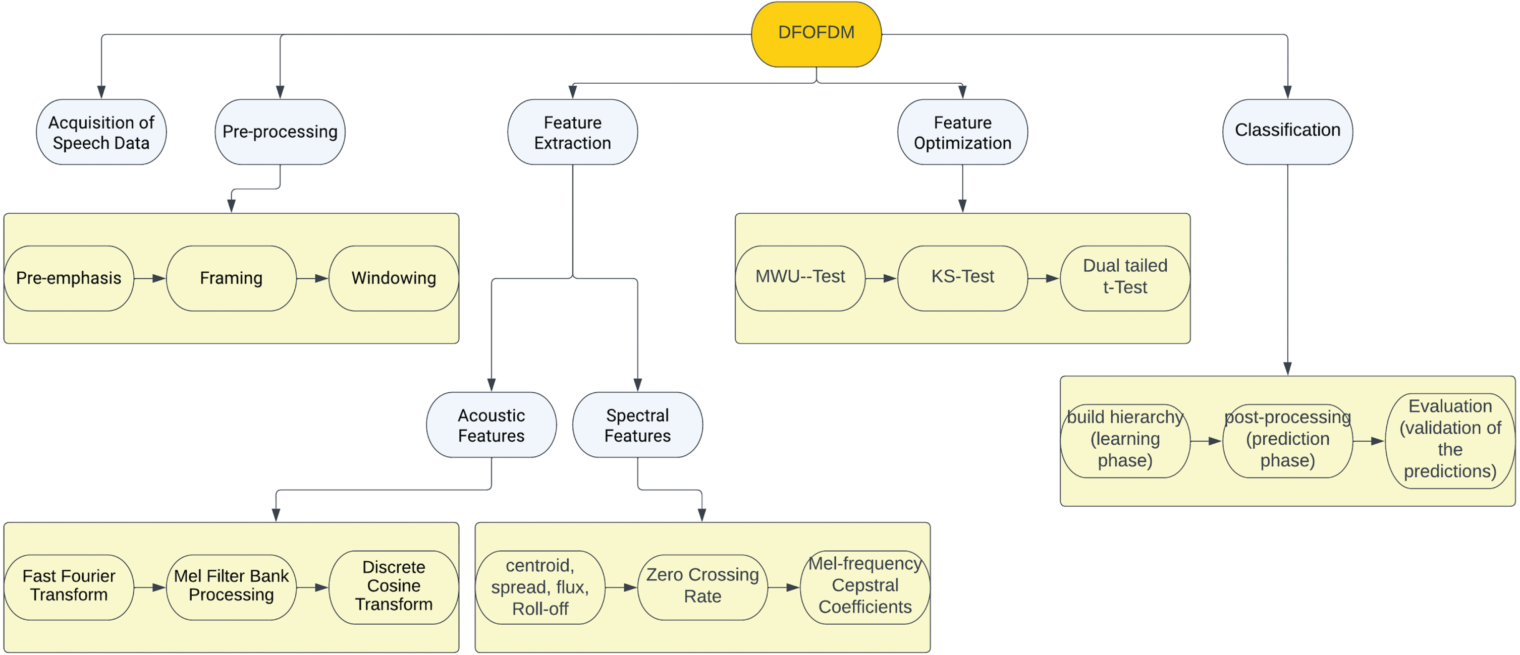
Flowchart for the DFOFDM.

In order to combine diversity measures under proposed fusion technique, the proposal employed the “Kolmogorov–Smirnov test [40]”, the “Mann–Whitney U Test [41]”, and the “two-tailed t-test [42]”.The fusion of the “Kolmogorov–Smirnov test”, the “Mann–Whitney U Test”, as well as the “two-tailed t-test” represents an innovative method for optimal feature selection in emotion recognition from speech signals. This combination leverages the unique strengths of each “test-Kolmogorov-Smirnov’s” ability to compare cumulative distributions, Mann-Whitney U’s capability to determine if two samples are likely from the same population, and the two-tailed t-test’s focus on comparing meansto robustly evaluate the diversity of features across different emotional states. This ensemble of tests enhances the discriminatory power of the features selected, likely leading to a more accurate and generalizable model for recognizing emotions in speech signals.

The new DFOFDM model is systematically compared to the prior techniques in the important areas of “speech emotion recognition (SER)” in Table 2. In terms of Feature Selection, DFOFDM integrates the strength of diversity measures and the Cuckoo Search algorithm, leading to optimal feature selection, which contrasts with the other techniques that often neglect feature optimization. Model Training is another distinguishing point, with DFOFDM utilizing both acoustic and spectral features and embedding diversity measures for optimal feature selection, a noticeable advantage over many traditional methods that fail to account for feature optimality and noise resilience. The use of Metaheuristic Search Techniques is common in both; however, DFOFDM specifically leverages the Cuckoo Search technique, facilitating a balance of local and global searches. Crucially, DFOFDM efficiently handles Label Imbalances, delivering more consistent results across varied emotion labels, a common challenge overlooked by many previous models. Performance on Real-world Data and Classifier Training specifics for DFOFDM are not explicitly stated in the table. However, it underscores that many previous models often struggle with real-world, noisy voice data, and they commonly use machine learning techniques like kNN, decision trees, and SVM for classifier training, with some incorporating deep learning.

Table 2

Comparative Analysis of DFOFDM and Previous Approaches in Speech Emotion Recognition

Factor	DFOFDM	Previous Approaches
Feature Selection	Uses a fusion of diversity measures “(KS-Test, MWU-test, and dual-tailed t-test)” and “Cuckoo Search” for optimal feature selection	Relies on Genetic Algorithms, Ant-Colony, particle swarm optimization, and NSGA II for feature selection, but overlooks optimization of features in some cases
Model Training	Employs acoustic and spectral features of the audio signal; incorporates diversity measures to select optimal features, and uses a Cuckoo Search-based classification approach	Uses a wide range of approaches, including “CNN”, “SVM”, “DCNN” with rectangular kernel, Ensemble Softmax regression model, but often does not address optimality of feature selection and noise resilience
Use of Metaheuristic Search Techniques	Utilizes Cuckoo Search, a metaheuristic technique that combines local and global searches for feature selection	Many studies use metaheuristic techniques such as Genetic Algorithms and Cuckoo Search, often combined with rough sets or Binary CS for feature selection
Handling of Label Imbalances	Addresses the challenge of label imbalances effectively with the proposed feature optimization strategy	Label imbalances often lead to unsteady accuracy rates across various emotion labels
Classifier Training	Using acoustic and spectral features	Most SER studies train kNN, decision trees, and SVM using acoustic features, with some recent research incorporating deep learning for feature extraction and classification

3.1 Speech signals and respective features

Speech signals are sound waves created by people speaking. These signals contain detailed information about the speaker’s emotional state, as is depicted in Fig. 2, as well as information about their identification, background, and even their physical health. They are frequently represented as one-dimensional time-series data that may be processed and analysed in a variety of ways for a variety of purposes, including automatic “speech recognition, speaker identification, emotion recognition, and health monitoring.” Acoustic features and spectral features are two examples of the several categories into which the characteristics of speech signals may be separated. These categories can offer various viewpoints on the information contained in the speech.

Fig. 2

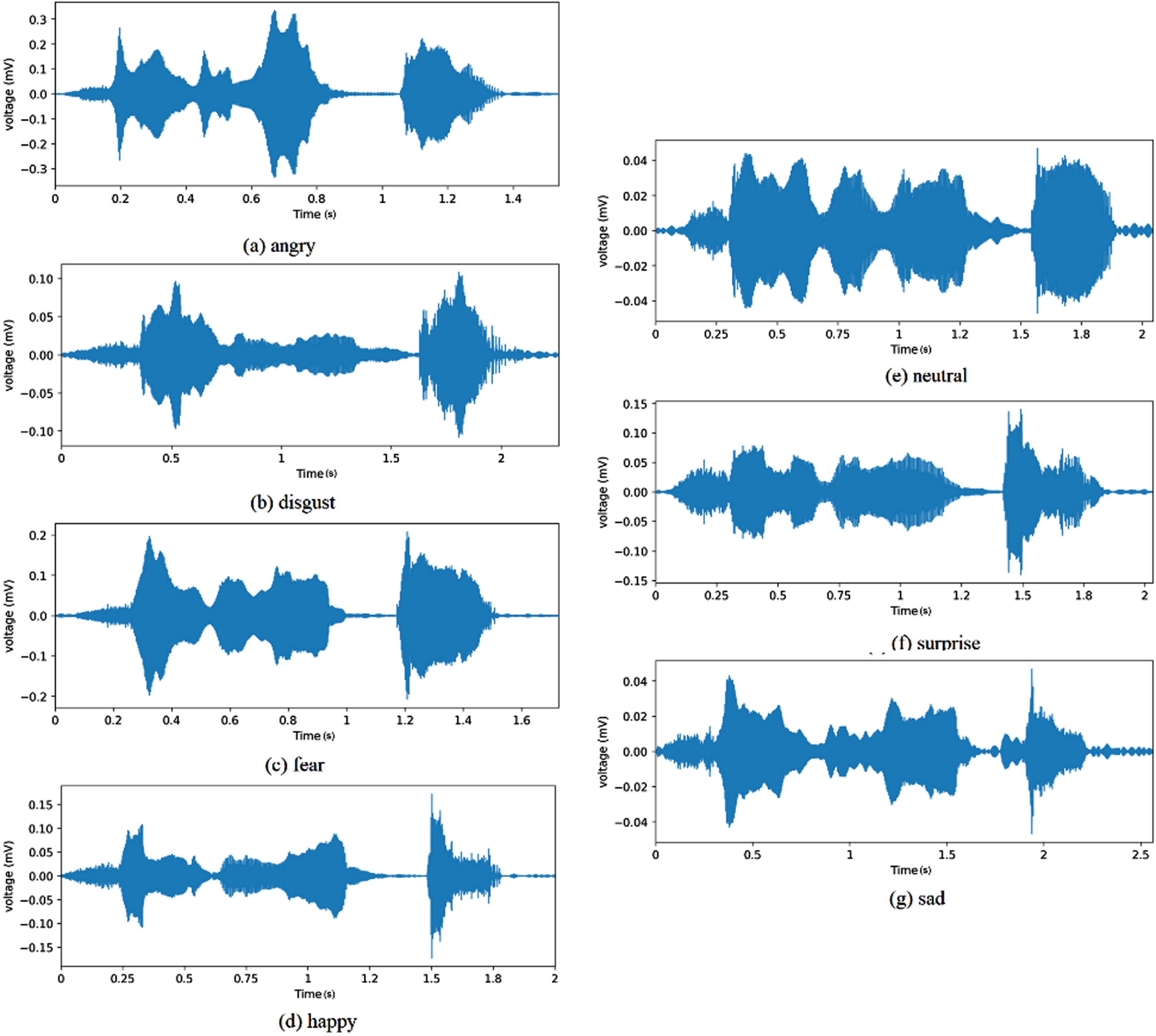
Visual representation of the different emotions as speech signals.

3.1.1 Acoustic features

The main elements that are extracted from the unprocessed audio waves are called acoustic features. They consist of peak values, zero-crossing frequency (a measure of noise content), amplitude, energy, and other time-domain characteristics. They also consist of formants (resonant frequencies of the vocal tract), pitch (the perceived fundamental frequency of a sound), as well as the length of speech segments. Acoustic features play a crucial role in speech analysis since they capture the basic temporal aspects of the audio stream and are frequently employed as a first step.

3.1.2 Spectral features

These characteristics are generated from the voice signal’s frequency content. They are often produced by converting a time-domain speech input into a frequency-domain signal using the Fourier Transform or other similar transformations like the “Mel-Frequency Cepstral Coefficients (MFCCs)” or “Linear Predictive Coding (LPC)”. Phonemes (individual sounds) are the building blocks of language, and their distinctive sonic fingerprints may be revealed by analysing spectral aspects. The spectral centroid, which is the centre of mass within the spectrum, the spectral flux, which measures the pace at which the spectrum changes, and the spectral roll-off, which identifies the range of frequencies below which a specific proportion of the total spectrum’s energy is present, are common spectral properties.

These characteristics are essential for speech emotion identification because they allow for the detection of minute variations in speech signals that are linked with various states of emotion. For instance, angry speech might be characterized by higher energy and a wider pitch range compared to neutral speech, while sadness might be associated with lower energy and a narrower pitch range. Thus, by analyzing these features, We can create models to categorise or forecast a speaker’s emotional state based on their speech cues.

3.2 Feature extraction

3.2.1 Acoustic features

The process of acoustic feature extraction is a fundamental part of speech signal processing and is usually conducted in several steps. Here, we will discuss it in the context of (MFCCs) extraction, which is one of the most popular collection of characteristics for speech as well as audio analysis.

1. Frame the signal: The continuous voice stream is divided into brief frames, generally 20–30 ms in duration. The reason for this is that speech is assumed to be stationary on this short time scale but not on a much larger scale. The frames can be expressed as: (Equation 1) $s_{i_{\left(n\right)}}=s_{\left(n+\mathit{iR}\right)},\mathit{for}0<=n<N$(1)

Where:

s_(n)is the original signal,

N is the length of the frame (e.g., 25 ms),

i is the frame index, and

R is the frame shift or frame stride (e.g., 10 ms). This allows the frames to overlap, which is common in speech analysis.

2. Apply window function: A window function w_(n) to reduce the signal discontinuity at the start and end of each frame, (typically a Hamming window) is added to each frame. (Equation 2) $s_i{w}_{\left(n\right)}=s_{i\left(n\right)}*w_{\left(n\right)}$(2)

3. “Fast fourier transform (FFT)”: Each windowed frame is given a Fast Fourier Transform in order to acquire the spectrum. (Equation 3) $S_{i\left(k\right)}=\mathit{FFT}\left\{s_i{w}_{\left(n\right)}\right\}$(3)

4. Mel filter bank processing: To produce a spectral form that more closely resembles the response of the human auditory system, the spectrum is run through a series of Mel-scale filters. The Mel filter bank’s output can be characterised as: (Equation 4) $m_{i\left(j\right)}={\mathit{sum}}_{\left\{k=0\right\}}^{\left\{N-1\right\}}{\parallel S_{i\left(k\right)}\parallel }^2*H_{j\left(k\right)}$(4)

Where:

∥S_i(k) ∥ ² is the power spectrum,

H_j(k) is the j ^th Mel filter,

N is the frame’s length, and

j Vary depending 1 on the Mel filter bank’s filter count (20–40, for example).

5. Discrete cosine transform (DCT): Finally, a “discrete cosine transform (DCT)” is applied to the log-Mel spectrum to yield the final set of “Mel-frequency cepstral coefficients (MFCCs)”. (Equation 5) $c_{i\left(n\right)}={\mathit{sum}}_{\left\{j=0\right\}}^{\left\{M-1\right\}}log\left(m_{i\left(j\right)}\right)*cos\left[\left(p_i/N\right)*\left(j+1/2\right)*n\right]$(5)

Where:

log(m_i(j)) is the log-Mel spectrum,

M is the number of filters in the Mel filter bank,

N is the length of the frame, and

c_i(n) for n = 0, . . . , N - 1 are the MFCCs.

Typically, only the first few MFCCs (e.g., 12–13) are used in speech recognition as they contain most of the speaker-specific information. The higher order coefficients represent noise and other less relevant information.

3.2.2 Spectral features

The process of spectral feature extraction from speech signals typically involves calculating spectral features such as Spectral Roll-off, Spectral Spread, Spectral Centroid, Spectral Flux, “Zero Crossing Rate (ZCR)”, and “Mel-frequency Cepstral Coefficients (MFCC)”. Let’s consider a windowed signal x (n) in the time domain, where n ranges from 0 to N - 1 (N being the size of the window). We assume that the “discrete Fourier Transform (DFT)” of x (n) is X (k), where k ranges from 0 to N - 1. Below are the mathematical definitions of these spectral features:

1. “Spectral centroid (SC)”: It indicates the “center of mass” of the spectrum and is computed as: (Equation 6) $\mathit{SC}=\frac{{\sum }_{k=1}^{\left|X\right|}\left(k*\parallel X\left(k\right)\parallel \right)}{{\sum }_{k=1}^{\left|X\right|}\left(\parallel X\left(k\right)\parallel \right)}$(6)

2. “Spectral spread (SS)”: It measures the “bandwidth” of the spectrum and is calculated as: (Equation 7) $\mathit{SS}=\mathit{sqrt}\left(\frac{\left({\sum }_{k=1}^{\left|X\right|}{\left(k-\mathit{SC}\right)}^2*\parallel X\left(k\right)\parallel \right)}{\left({\sum }_{k=1}^{\left|X\right|}\parallel X\left(k\right)\parallel \right)}\right)$(7)

3. “Spectral flux (SF)”: Calculated as, it gauges how quickly a signal’s power spectrum is shifting: (Equation 8) $\mathit{SF}=\mathit{sqrt}\left(\left(\frac{1}{2n}\right)*\sum _{k=1}^{\left|X\right|}{\left(\parallel X\left(k\right)\parallel -\parallel X_{\mathit{prev}}\left(k\right)\parallel \right)}^2\right)$(8) where X _prev  (k) is the spectrum of the previous frame.

4. “Spectral roll-off (SR)”: It measures the frequency below which a specified percentage (e.g., 85% or 95%) of the total spectral energy lies. SR is calculated as the lowest k for which: (Equation 9) $\frac{\left({\sum }_{i=0}^{\left|X\right|}k\parallel X\left(i\right)\parallel \right)}{\left({\sum }_{i=0}^{\left|X\right|}N-1\parallel X\left(i\right)\parallel \right)}>=\mathit{Threshold}$(9)

5. “Zero crossing rate (ZCR)”: It gauges how quickly the signal’s indication changes. This is not a spectral feature but is often used in conjunction with spectral features as: (Equation 10) $\mathit{ZCR}=\left(1/\left(2n\right)\right)*\sum _{n=1}^{\left|X\right|}N\parallel \mathit{sign}\left[x\left(n\right)\right]-\mathit{sign}\left[x\left(n-1\right)\right]\parallel$(10) where sign is a function that produces –1 for negative numbers, 0 for zero, and 1 for positive values.

6. “Mel-frequency cepstral coefficients (MFCCs)”: These coefficients make up an MFC as a whole. They come from the following:

Take the absolute DFT signal log value.

Pass the signal through Mel-filters, which are triangular filters that mimic the human auditory system’s non-linear frequency resolution.

Take the “Discrete Cosine Transform (DCT)” energies of the log filter.

3.3 Optimal feature selection

This section discusses feature optimization using a suggested fusion technique that ensembles different metrics of distribution diversity. This is because distribution measurements permit the differentiation of two distributions. The choice of the “Mann-Whitney U Test”, the “Kolmogorov-Smirnov (KS) Test”, and the “two-tailed t-test” as diversity assessment measures to evaluate the diversity between two imbalanced data vectors is justified by their unique and complementary characteristics.

“Mann-Whitney U Test (MWU-Teest)”: This test’s flexibility stems from the fact that it is non-parametric and so does not presume anything about the data’s distribution. It determines if there is a meaningful distinction between two independent sets of non-normally distributed data. In other words, it compares the distributions of two groups and can identify if one distribution is stochastically larger than the other, making it suitable for comparing imbalanced data vectors.

“Kolmogorov-Smirnov Test (KS-Teest)”: This is another non-parametric test used to compare two cumulative distributions. If two samples are taken from the same distribution, it can be used to identify that. For imbalanced datasets, it provides a valuable measure of how much one cumulative distribution function deviates from another.

“Dual Tailed T-Test”: When comparing the means of two groups, a two-tailed t-test is performed to evaluate whether there are any significant differences. The “two-tailed” nature of the test means that it considers deviations in both directions— whether one mean is either significantly greater or significantly less than the other. This can be particularly useful in situations where we don’t have a specific expectation about the direction of the difference between the groups.

By combining these three tests, it’s possible to assess the diversity of data vectors in multiple ways— from the perspective of their distributions (KS and Mann-Whitney U) as well as their means (two-tailed t-test). This provides a more comprehensive assessment of diversity than any single test would alone. This fusion of tests could be particularly effective in the context of imbalanced data, which could exhibit diversity in both the central tendency and the distribution of the data.

In contrast to current models, for each class of emotions, speech signals will be segmented in to multiple spectrograms representing the voiced portion of the corresponding speech signal. Further, extracts all acoustic and spectral features. The distribution of the acoustic and spectral features of the speech signal will be considered as a vector. Set of all these vectors of are treated as a matrix of the corresponding class of emotion. Such that each column representing the feature vector of each speech signal belonging to the same emotion class. Additionally, the proposed fusion of diversity measures shall be used to estimate the diversity between each column of a emotion class and the same column of the other emotion class’s matrix. If the resulting diversity exceeds the specified threshold, the column is said to have the ideal properties of the related class of emotion.

Find the optimum features for each set D _j of samples denoting j ^th label in comparison to the corresponding set {D _k ∃ k ≠ j }. If the samples projected to the {D _k ∃ j ≠ k } set’s feature diversity with the samples projected for same feature x _i in all other sets {D _k ∃ k ≠ j }, a feature x _i is optimum for each set D _j . The procedure will assess the diversity-weight of each set {D _k ∃ j ≠ k }, the probable closeness observed (0 ⩽ p ⩽ 1), for each feature x _i of the set D _j . The following explanation depicts the statistical model to identify optimal characteristics.

${\forall }_{i=1}^{\left|X\right|}\left\{x_i\left(\in X\right)\right\}$ Begin // for each feature

${\forall }_{j=1}^{\left(n-1\right)}\left\{\left[x_i^j\right]\left(\in D_j\right)\right\}$ // Begin

dw_{x i ⇒D j}  = 1// the cumulative diversity of the feature x _i towards the class of emotion D _j

${\forall }_{k=1}^{\left(n\right)}\left\{\left[x_i^k\right]\left(\in D_k\right)\exists k\ne j\right\}$ // Begin

$\begin{array}{c}{p}_{\mathit{mwu}}\leftarrow \mathit{MWUtest}\left(\left[x_i^k\right],\left[x_i^j\right]\right)\\ p_{\mathit{ks}}\leftarrow \mathit{KStest}\left(\left[x_i^k\right],\left[x_i^j\right]\right)\\ p_{\mathit{dt}}\leftarrow \mathit{DTtest}\left(\left[x_i^k\right],\left[x_i^j\right]\right)\\ \end{array}\}$ // estimating the diversity of the feature x _i among the sets D _j , D _k

d (x _i ) _{D j ←      →D k}  ← dτ// the d (x _i ) _{D j ←      →D k} (diversity) is being set to dτ

if ((p _ks  ∨ p _mwu  ∨ p _dt ) < pτ) Begin// is the probability threshold pτ higher than one of the similarity scores (p _ks , p _mwu , p _dt )

d (x _i ) _{D j  ←      →D k}  ← (p _mwu  ⊗ p _ks  ⊗ p _dt ) //the distribution diversity d (x _i ) _{D j  ←      →D k} between the values representing the feature x _i and existing in sets D _j   ←        → D _k has been discovered.

End

dw_{x i ⇒D j}  ← d (x _i ) _{D j  ←      →D k}  ⊗ dw_{x i ⇒D j}

End

(fD _j  ← x _i  ∃ dw_{x i ⇒D j}  ⩾ dτ) // move feature x _i to the set fD _j , if diversity-weight dw_{x i ⇒D j} not less than the stated diversity-threshold dτ

End

End

// prune the datasets of diversified labels//

${\forall }_{j=1}^{\mathit{lc}}{\forall }_{i=1}^{\left|X\right|}\left\{x_i\exists x_i\in X\wedge x_i\notin f{D}_j\right\}$ Begin // for each featurex _i of the class label j

{D _j  } ∖ [x _i ]// discards feature values [x _i ]listed in set D _j

End

// n-grams of each class (label)//

${\forall }_{j=1}^{\mathit{lc}}{\forall }_{i=1}^{\left|D_j\right|}\left\{r_i\left(\in D_j\right)\right\}$ Begin// for each record r _i of that setD _j

nG _j  ← (nG _j  ∪ nGrams (r _i ))// discovering n-grams and moving resultant unique n-grams to the set nG _j that is not belongs to the set nG _j

End

Further, determines the positive, negative probability of each class label, decision support, as well as purity of n-grams occurrence in the set represented by respective class label.

${\forall }_{j=1}^{\mathit{lc}}{\forall }_{i=1}^{\left|n{G}_j\right|}\left\{n{g}_i\left(\in n{G}_i\right)\right\}$ Begin //each of the n-grams of that label j

${\mathit{ng}}_{\left[j,i\right]}^{+}=\left({\sum }_{k=1}^{\left|D_j\right|}\left\{1\exists n{g}_i\subseteq r_k\wedge r_k\in D_j\right\}\right)*{\left(\left|D_j\right|\right)}^{-1}$ // discovers the ${\mathit{ng}}_{\left[j,i\right]}^{+}$ (positive probability) of each n-gram ng _i towards the class label j

${\mathit{ng}}_{\left[j,i\right]}^{-}=\frac{1}{\left|D_j\right|}\left(\left|D_j\right|-\left(\left|D_j\right|*{\mathit{ng}}_{\left[j,i\right]}^{+}\right)\right)$ //discovers negative probability ${\mathit{ng}}_{\left[j,i\right]}^{-}$ of each n-gram ng _i towards the class label j

${\mathit{ng}}_{\left[j,i\right]}^w=1-\left(\begin{array}{c}\left(\left(1-{\mathit{ng}}_{\left[j,i\right]}^{+}\right)*{\mathit{ng}}_{\left[j,i\right]}^{+}\right)+\\ \left(\left(1-{\mathit{ng}}_{\left[j,i\right]}^{-}\right)*{\mathit{ng}}_{\left[j,i\right]}^{-}\right)\\ \end{array}\right)$ //discovers purity of each n-gram ng _i towards the set D _j , which has been derived by Gini impurity estimation [43]

End

End

${\forall }_{j=1}^{\mathit{lc}}{\forall }_{i=1}^{\left|n{G}_j\right|}\left\{n{g}_i\in n{G}_i\right\}$ Begin // for each label j, for each n-gram of that label

ip_[j,i] = 1 // the total impurity ip_[j,i] is set to 1(maximum)

${\forall }_{k=1}^{\mathit{lc}}\left\{n{g}_i\left(\in n{G}_k\right)\exists j\ne k\right\}$ Begin // for each label j, for each n-gram of that label

$i{p}_{\left[j,i\right]}=i{p}_{\left[j,i\right]}*{\mathit{ng}}_{\left[k,i\right]}^w$ // updating the impurity ip_[j,i] of each n-gram ng_[j,i]

End

${\mathit{ng}}_{\left[j,i\right]}^{\mathit{dw}}\leftarrow {\mathit{ng}}_{\left[j,i\right]}^w-1+i{p}_{\left[j,i\right]}$ // the decision weight ${\mathit{ng}}_{\left[j,i\right]}^{\mathit{dw}}$ of each n-gram ng_[j,i]with regard to the set (label) D _j

$\left(\left(n{G}_j\setminus n{g}_i\right)\exists \left({\mathit{ng}}_{[j,i]}^{\mathit{dw}}<d\tau \right)\right)$ // discarding the n-gram ng _i of the set D _j , if and only if the decision weight ${\mathit{ng}}_{\left[j,i\right]}^{\mathit{dw}}$ of each n-gram ng_[j,i] with regard to the set (label) D _j is lower than the threshold for the decision weight

End

3.3.1 “MWU-test (Mann-Whitney U Test)”

This isnon-parametric method that gauges diversity scope between two distributions, which makes no assumptions about score distribution. However, various assumptions are made, such as the randomness of the observation selected from the population, the independence of the observations and bilateral independent, and the use of an arbitrary measuring tool. As an alternative, use this non-parametric test to an independent t-test. It’s used to see if two samples are from the same population or if the given observations are larger than the other observations. The following is a description of the MWU-Test implementation process:

Let the pair of vectors d₁, d₂ have been given to the MWU-Test as input, which scales the diversity among the distributions of the given two vectors as follows,

According to set theory principle, perform union operation on given two vectors. d₁, d₂. in to resultant vector d. Further, arrange the elements of the vector d in their incremental order and consider each element’s index as the rank of the corresponding element. The notation I represents the list of ordered ranks of the elements of the vector d. Let the notations I₁, I₂ represents the ranks of the elements listed in vectors d₁, d₂ in respective order. The rank of the elements having more than one entry will represent by their average of the rank. Further, discovers the sum of all entries in the list I₁ as SI₁ and also discovers the sum of all entries in list I₂ as SI₂, which will be used further to obtain rank sum thresholds SIT₁, SIT₂ of the vectors d₁, d₂ as follows: (Equation 11), and (Equation 12) $\mathit{SI}{T}_1=S{I}_1-{\left(\left|d_1\right|\times (\left|d_1\right|+1)\right)}^{-2}$(11) $\mathit{SI}{T}_2=S{I}_2-{\left(\left|d_2\right||\left(\left|d_2\right|+1\right)\right)}^{-2}$(12)

// the notations |d₁|, |d₂| denotes the size of the respective vectors d₁, d₂.

The notation SIT represents the rank-sum threshold of the all entries listed in both vectors d₁, d₂, which is the aggregate of SIT₁, SIT₂ that measured as follows. (Equation 13) $\mathit{SIT}=\mathit{SI}{T}_1+\mathit{SI}{T}_2$(13)

In order to discover z-score [44], measure the mean m _RST as well as deviation d _SIT as stated in (Equation 14) and (Equation 15): $m_{\mathit{SIT}}=\left(0.5\times \mathit{SIT}\right)$(14)

$\begin{array}{cc}\hfill & d_{\mathit{SIT}}=\sqrt{\frac{\left|d_1\right|*\left|d_2\right|*\left(\left|d\right||+1\right)}{\left|d\right|}}\hfill \\ \hfill & -\sqrt{\frac{\left|d_1\right|*\left|d_2\right|}{\left|d\right|}\left(\left(\left|d\right|+1\right)-\sum _{i=1}^k\frac{t_i^3-t_i}{\left|d\right|*\left(\left|d\right|-1\right)}\right)}\hfill \end{array}$(15)

The notation k signifies the count of separate rankings, and notation t _i stands for the total elements with the same rank.

Afterwards, the z-core evaluates as followsin (Equation 16): $z={\left(\mathit{SIT}-m_{\mathit{SIT}}\right)}^{-d_{\mathit{SIT}}}$(16)

Then find the p-value in the z-table [45]. The greater p-value that compared to given probability threshold denotes that the input vectors d₁, d₂ are diversely distributed, if not, the vectors are not distributed diversely.

3.3.2 KS-test

The distance metric, dubbed the “Kolmogorov-Smirnov test (KS-test) [40]”, is employed to quantify the diversity of two distributions. Additionally, this metric does not require a great deal of information regarding the distribution type of data, which differentiates it from previous methods for detecting distribution variety. The KS-test statistic scales the distance among the observation’s empirical distribution and the reference distribution’s cumulative distribution. Using the null-hypothesis that the observation has been taken from the observation estimate or that the observations have been taken from the respective distribution, the null-distribution of this measure is derived. A null-distribution evaluated in one-observation cases could be continuous, finite, or mixed. In the two-observation scenario, the null-hypothesis considers a linear but unbounded distribution. Two sampling tests can be done to accommodate for disruption, heterogeneity, as well as reliance between observations. The K–S test compares two observations, which is sensitive to changes in both position as well as form of the estimated cumulative distribution of the two observations.This test could be used to assess fitness. In the instance of evaluating distribution normality, observations are normalized and contrasted with a normally distributed observation. This is comparable to changing the reference distribution’s variance as well as adding a mean to the estimated observations, which modifies the test statistic’s null-distribution. The following procedure is used to apply “KS-Test”:

Let the notations v _a and v _b be two vectors. The following is how the KS-Test will be used to compare the populations of two vectors that are same or distinct:

The technique begins by evaluating the cumulative values Ag (v _a ) , Ag (v _b ) of vectors v _a , v _b . The cumulative-ratio of elements of vectors v _a , v _b is then predicted. $\begin{array}{cc}\hfill & \mathit{pr}=0\hfill \\ \hfill & \underset{i=1}{\overset{\left|v_j\right|}{\forall }}\left\{e_i\in v_j\right\}\mathit{begin}\hfill \\ \hfill & \mathit{pr}=\left(e_i*\mathit{Ag}{\left(v_j\right)}^{-1}\right)+\mathit{pr}\hfill \\ \hfill & C{R}_{v_j}\leftarrow \mathit{pr}\hfill \\ \hfill \&\mathit{end}& \hfill \end{array}$(17)

The notation denotes each member of a vector v _j in (Equation 17). The notation CR _{v j} denotes the set that contains aggregated ratios of elements present v _j . The notation pr denotes the cumulative ratio of the recently departed element in iterative process; the notation Ag (v _j ) denotes the aggregate of values listed in vector v _j ; and the notation Ag (v _j ) denotes the set that comprises cumulative ratios of elements presented v _j . As a result, the technique for finding aggregate ratios of values listed in vectors v _a , v _b as the sets CR _{v a} , CR _{v b} in respective order. Further, uncovers the positive definite variance of “aggregated ratios” of elements presented at an identical index both in v _a , v _b vectors.

${\forall }_{i=1}^{max\left(\right|C{R}_{v_a}|,|C{R}_{v_b}\left|\right)}\left\{\left(c_i\left(v_b\right)\left(\in C{R}_{v_b}\right)\right)\wedge \left(c_i\left(v_a\right)\left(\in C{R}_{v_a}\right)\right)\right\}$ , Begin // each of the values indexed at i in CR _{v a} , CR _{v b} $A{D}_{C{R}_{v_a}\leftarrow \to C{R}_{v_b}}\leftarrow \left\{\sqrt{{\left(c_i\left(v_a\right)-c_i\left(v_b\right)\right)}^2}\right\}$

// the absolute variance AD of cumulative ratios reported in sets CR _{v a} , CR _{v b} at index i that is then placed in set AD_{CR v a  ←      →CR v b} .

End

Afterwards, determine d-stat, which will be the highest value stored in the set AD_{CR v a  ←      →CR v b} . Determine the d-critic of Ag (v _a ) , Ag (v _b ) using KS-Table for “degree of probability-threshold”.The distributions of two vectors are the same if and only if d-stat is higher than the stated d-critic.

3.3.3 “Dual tailed variance test”

A “dual-tailed test”, also known as a t-test, was used as the scale for evaluating distribution diversification in the suggested fusion method. There are two approaches to calculate the statistical validity of a feature derived from a dataset using a test statistic: a “one-tailed t-test” and a “two-tailed t-test”. One of the most common situations in which two-tailed tests can be used in research is when a test-score takers is within or falls outside of an acceptable range of values. The research hypothesis is rejected against the null-hypothesis if the estimation occurs in the crucial aspects of the experiment. Assuming that the predicted value can only deviate in one way, a one-tailed t-test becomes acceptable. Based on whether it’s higher than or less, a different hypothesis will take precedence over a null hypothesis in the one-sided critical areas. Because of the limited size of the extreme regions of distributions wherein observations results null-hypothesis rejection and generally “tail off” towards zero as in the normally distributed dataset. The diversity between featured values (y-coordinates) projected for a feature (x-coordinate) of records with various labels can be determined using this method. Recent developments in the dual t-test [42, 46] have encouraged us to incorporate it into the fusion method we propose. In (Equation 18) the diversity of distributions of two vectors {r _i , r _j ∃ i ≠ j } is estimated as follows: $f\left(r_i,r_j\right)=\frac{\left(\mu \left(r_i\right)-\mu \left(r_j\right)\right)}{\left(\sqrt{{\sigma }_{\left(r_i\right)}+{\sigma }_{\left(r_j\right)}}\right)}$(18)

The diversity of distributions of the vectors {r _i , r _j ∃ i ≠ j } is determined by the operator f (r _i , r _j ) in eq-10. The average value of the respective distributions are represented by the notations μ (r _i ) , μ (r _j ), and the deviation of the corresponding vector distributions is represented by the notations σ_{(r i )}, σ_{(r j )}. The diversification of the distributions is defined as the ratio of the average difference between the vectors to the square root of the total of their variances.

The diversity that is less than the specified probability value (p-value) [44, 45], reflecting that the distributions are divergent.

3.4 The classifier

Engineering is increasingly using meta-heuristic algorithms that draw inspiration from nature. This work makes use of (CS). Despite eating the eggs of other birds to increase their chances of hatching, female cuckoos continue to lay eggs in nests. Some bird species prey on other bird species by laying eggs in their own nests. There have been three main types of brood parasitism: Thirdly, parasitism within the same species, namely of offspring. When a host bird discovers foreign eggs in its nest, it might choose to either abandon the eggs or move the nest to a safer location.

The algorithm is defined by the unusual egg-laying and breeding behaviours of the cuckoo. If the host animal realises that the eggs it is caring for aren’t its own, it will either reject the offending offspring or abandon the nest in search of suitable nesting grounds. Three condensed, yet essential, characteristics make up the Cuckoo Search’s user-friendliness: High-quality eggs would be laid in the perfect nest and passed down to next generations. The overall number of host nests is constant, and either 0 or 1 hosts have reported finding a cuckoo’s egg. The host bird may react to these characteristics by rejecting the egg or abandoning the nest in favour of a fresh start. This ultimate state may be roughly estimated by looking at the ratio of old nests to new ones.

3.5 Classifier model

The classifier establishes the perch hierarchy representing each of the class labels in the training corpus, which was constructed on cuckoo search. There are several tiers in this structure, and at least one perch shall be found at each level. There are n-gram representations of acoustic and spectral features on each perch in the hierarchy. The n-gram features on each level are the same size. If you look at the perches in a level, you can see the n-gram features that are smaller than the n-grams’ size that are shown there and bigger than the n-grams’ size features shown there. In the next part of the learning phase, the computer places unique n-grams of features that correspond to each label of the perches of the hierarchy, so that the computer can figure out what each label means.

3.6 Class prediction phase

The process that predicts the test record tr ’sclass label is as follows.

Notation nG _tr denotes a set of distinct n-grams of size ranges from 1 to the est record tr ’s size |tr|.

foreach label j Begin

jF _tr  = 0 // test record tr ’s fitness indicator $j{F}_{\mathit{tr}}=\sum _{i=1}^{\left|\mathit{tn}{G}_{\mathit{tr}}\right|}\left(\sum _{\mathit{idx}=1}^{\left|H_j\right|}\left(\sum _{k=1}^{\left|l_{\mathit{idx}}\right|}\left\{\begin{array}{c}{\mathit{tng}}_{\left[j,i\right]}^{\mathit{dw}}\exists \\ \mathit{tn}{g}_{\left[j,i\right]}\in p_k\wedge \\ p_k\in l_{\mathit{idx}}\wedge \\ l_{\mathit{idx}}\in H_j\\ \end{array}\right\}\right)\right)$(19)

//Aggregating all n-gram decision-weights of test record tr in relate to label j’s hierarchy H _j . ${\mathit{jep}}_{\mathit{tr}}^{\mathit{dw}}=j{F}_{\mathit{tr}}\times {\left(\sum _{\mathit{idx}=1}^{\left|H_j\right|}\left|l_{\mathit{idx}}\right|\right)}^{-1}$(20)

//Exploring the ${\mathit{jep}}_{\mathit{tr}}^{\mathit{dw}}$ (empirical probability) of said decision-weights in relation to the hierarchy H _j of the class label j.

${\mathit{jd}}_{\mathit{tr}}^{\mathit{dw}}={\sum }_{i=1}^{\left|\mathit{tn}{G}_{\mathit{tr}}\right|}\left({\sum }_{\mathit{idx}=1}^{\left|H_j\right|}\left({\sum }_{k=1}^{\left|l_{\mathit{idx}}\right|}\left\{\begin{array}{c}\sqrt{{\left({\mathit{jep}}_{\mathit{tr}}^{\mathit{dw}}-{\mathit{tng}}_{\left[j,i\right]}^{\mathit{dw}}\right)}^2}\exists \\ \mathit{tn}{g}_{\left[j,i\right]}\in p_k\wedge \\ p_k\in l_{\mathit{idx}}\wedge l_{\mathit{idx}}\in H_j\\ \end{array}\right\}\right)\right)\times {\left({\sum }_{\mathit{idx}=1}^{\left|H_j\right|}\left|l_{\mathit{idx}}\right|\right)}^{-1}$ //Measures the deviation ${\mathit{jd}}_{\mathit{tr}}^{\mathit{dw}}$ of the decision-weights.

End

In order to assess every label’s accuracy j, we will calculate the empirical probability ${\mathit{jep}}_{\mathit{tr}}^{\mathit{dw}}$ of each label and the corresponding deviation ${\mathit{jd}}_{\mathit{tr}}^{\mathit{dw}}$ of the decision-weights witnessed for all potential n-grams

3.7 Estimating the labellingscope

Class label of the test record tr is being estimated as follows

${\forall }_{k=1}^{\left|\mathit{lc}\right|}\left\{k\exists 1⩽k⩽\mathit{lc}\right\}$ // Begin //for each label k

$i{p}_k=1-{\prod }_{j=1}^{\left|\mathit{lc}\right|}\left\{\left({\mathit{jep}}_{\mathit{tr}}^{\mathit{dw}}-{\mathit{jd}}_{\mathit{tr}}^{\mathit{dw}}\right)\exists j\ne k\right\}$ //discovers class label’s impurity ip _k

$f_k^{\mathit{tr}}=\left({\mathit{kep}}_{\mathit{tr}}^{\mathit{dw}}-{\mathit{kd}}_{\mathit{tr}}^{\mathit{dw}}\right)-i{p}_j$ // fitness of the label k with regard to record tr

End

Finally, it predicts the label that indicates the emotion of the given test record tr as follows, with regard to each label j, based onthe empirical probability ${\mathit{jep}}_{\mathit{tr}}^{\mathit{dw}}$ , respective deviation ${\mathit{jd}}_{\mathit{tr}}^{\mathit{dw}}$ , and the fitness $f_j^{\mathit{tr}}$ of decision-weightstowards the corresponding label, the class label is being predicted. The Likert scale [47] is being applied to assess the class label fitness.

There is a pecking order of importance given to the empirical probability, the deviation, and the test record’s suitability to the label. The Likert Scale assigns a value of 1 to the least important factor and raises the bar by 1 for each succeeding factor. The parameters’ normalized index values are multiplied by the test record’s label to reveal the degree of agreement between the two.

The range of the index will be 1, 2, as well as 3, with the values 1 indicating the most deviation, 2 representing the greatest empirical likelihood, and 3 representing the greatest fitness. The following is an estimation of the degree to which the test record is related to the label ’j’.

${\forall }_{j=1}^{\left|\mathit{lc}\right|}\left\{j\exists \left(1⩽j⩽\mathit{lc}\right)\right\}$ // for each label j ${\mathit{cr}}_{\mathit{tr}}^j=1-\left(\left({\mathit{jd}}_{\mathit{tr}}^{\mathit{dw}}\right)*\left({\mathit{jep}}_{\mathit{tr}}^{\mathit{dw}}*(1-2^{-1})\right)*\left(f_j^{\mathit{tr}}*(1-3^{-1})\right)\right)$(21)

Therefore, it is concluded that the test record is most closely associated with the label j.

4 Experimental study

The study results that were carried out using the suggested approach and other modern methodologies are covered in this section. The description includes information about the dataset, and hardware as well as software specifications that were used, as well as an estimation of performance using statistical metrics. Python was used to implement the proposed approach [48], and the code was built using the Python editor “PyCharm” [49]. In this regard, I5-7^th gen Intel processor with 32 GB of memory and a 1TB storage was considered for the hardware requirements.

4.1 The data

The “TESS (Toronto Emotional Speech Set)” [50] was utilised in the test study because it contains multiple samples of audio representing human emotions such as “disgust, fear, happy, sad, angry, neutral, and surprise” (total seven emotion types). The dataset contains between 390 and 400 records for each of these emotion labels. The following Table 3 summarizes the dataset’s statistics. The speech signals given as input represent a range of emotions and are framed by 200 words spoken in English by a range of people experiencing a range of emotions.

Table 3

The number of input speech signals labeled with a variety of human emotions

Label	Surprise	Sad	Angry	Fear	Neutral	Disgust	Happy
input records count	393	392	396	399	398	399	400

4.2 Data processing

For each class of emotion, each mono wav file given as input is beingpartitioned into spectrogram and discovers voiced segments using scipy library [51]. Further, discovers all acoustic and spectral features using opensmile python library [52] which shall be considered as a row of the two-dimensional matrix of the corresponding class of emotions. Following data processing, there are matrices of feature values, each of which corresponds to one among the selectedemotion labels.

4.3 Performance analysis

The suggested method DFOFDM and the contemporary model TSLSL [37] were evaluated using assessment metrics associated with their respective confusion matrices (see Table 4 and Table 5). Testing as well as training corpora have been created from the labelled corpus of the given dataset. The training corpus contains 90% of the labelled records, while the remaining 10% has been used to evaluate the classification ability of presented and contemporary models. The given data records for the train and test phases are classified using seven distinct labels, as specified in the dataset description. In performance analysis, the metrics precision and recall/sensitivity were used to define accuracy in multi-label classification. In addition to the dependent metrics, the definition of micro-precision, micro-F-scale, micro-recall, as well as Prediction Accuracy yielded “F-score, weighted-precision, weighted-recall, but also weighted F-Score”, all of which represent the total classification performance in identifying the multi-class data.The F-score, recall (or sensitivity), as well as precision are common measures used to assess a classification model’s effectiveness. These measures are especially important when dealing with multi-label classification problems, because each instance may simultaneously belong to numerous classes.

Table 4

The confusion matrix for DFOFDM’s multi-label classification.

	Actual Label ⇓
		Angry	Disgust	Fear	Happy	Neutral	Sad	Surprise	PREDICTED LABEL COUNT⇓
Predicted Label ⇒	Angry	36	1	1	0	0	1	0	39
	Disgust	2	37	1	0	0	1	1	42
	Fear	0	1	35	0	2	1	1	40
	Happy	0	0	0	38	0	0	2	40
	Neutral	0	0	0	1	36	1	0	38
	Sad	0	1	1	0	2	35	0	39
	Surprise	2	0	1	1	0	0	35	39
ACTUAL LABEL COUNT ⇒		40	40	40	40	40	39	39

Table 5

Confusion matrix of TSLSL’s multi-label categorization

	Actual Label ⇓
		Angry	Disgust	Fear	Happy	Neutral	Sad	Surprise	PREDICTED LABEL COUNT⇓
Predicted Label ⇒	Angry	31	1	2	0	1	1	0	36
	Disgust	2	33	1	2	2	1	2	43
	Fear	1	1	30	0	3	1	1	37
	Happy	2	2	2	34	0	0	3	43
	Neutral	1	1	2	1	32	4	0	41
	Sad	1	1	1	2	2	31	0	38
	Surprise	2	1	2	1	0	1	33	40
ACTUAL LABEL COUNT ⇒		40	40	40	40	40	39	39

1. Precision: This is the percentage of all positive predictions produced by the model that are true positive predictions (i.e., examples that are accurately classified as belonging to a certain class). A model with high precision has a low false-positive rate and correctly recognises instances that correspond to a given class.

2. Recall/Sensitivity: Recall quantifies how many actual positive cases— that is, occurrences that genuinely fall within a given class— were accurately recognised by the model. A model that has a high recall is good at capturing instances of a given class and has a low false-negative rate.

3. F-score: The harmonic mean of recall and precision is the F-score. It acts as a single metric to reconcile the compromise between recall and precision. The F-score is highest at 1 (perfect recall and precision), and it is worse at 0.

4. One of the easiest machine learning metrics to understand is accuracy. It is determined by dividing the total number of forecasts by the number of accurate predictions the model made. It is, in other words, the proportion of accurate forecasts (including true positives and true negatives) to all cases considered. It is frequently stated as a percentage, with a greater number denoting better model performance.

In a multi-label classification job, the “micro-” and “weighted” variations of these metrics offer various methods for aggregating the metric values over several classes.

Micro-Precision, Micro-Recall, and Micro-F-score: These metrics calculate the average metric from the contributions of all classes. All classes are given equal weight when using micro-averaging, and the metric is produced globally by adding up all of the true positives, false negatives, and false positives.

Weighted-Precision, Weighted-Recall, and Weighted F-Score: These metrics resemble micro-averaged measures but also account for the unequal distribution of the classes. The number of true cases for each class is taken into consideration (the “weight”) with weighted-averaging since each class metric is computed individually and then added.

Prediction Accuracy: This is the ratio of the model’s correct predictions to all of its predictions. Prediction accuracy may not be a good indicator of performance in the context of multi-label classification since it does not take into account unbalanced classes or the possibility of any instance belonging to numerous classes.

These metrics provide an all-encompassing picture of how well a model performs in multi-label classification tasks. They enable the evaluation of the model’s precision, recall, and F-score, which measure how well it can distinguish between instances of each class and capture them all. They also shed light on the performance of the model across all classes, both overall (micro-averaging) and while taking into account class imbalances (weighted-averaging).

Multi-label classification using the suggested DFOFDM model is shown in Table 4 as a confusion matrix. The projected labels are in each row, while the actual labels are in each column. Cell counts reflect the number of times a given row was incorrectly assigned to a given column in the model’s predictions. For instance, the model accurately identified the emotion “Angry” 36 times, whereas “Disgust,” “Fear,” and “Sad” were all mispredicted once each. Each projected label’s total count is given in the row labelled “Predicted Label Count,” while each actual label’s total count is given in the column labelled “Actual Label Count.”

Table 5 The confusion matrix used by the current TSLSL model to conduct multi-label classification is shown in the Table 5. Similar to Table 4, each row and column correspond to the predicted as well as actual labels, respectively. The values in the cells represent how many times the TSLSL model made a specific prediction (row) for each actual label (column). For instance, the TSLSL model correctly predicted ‘Angry’ 31 times and misclassified it for ‘Disgust”, ‘Fear”, ‘Neutral”, and ‘Sad’ once each. The ‘Predicted Label Count’ row indicates the total number of times each label was predicted, and the ‘Actual Label Count’ column shows the total count for each real label.

Figure 3 provides a comparative representation of “True Positive (TP)” and “False Positive (FP)” rates for both the DFOFDM and TSLSL models, which are derived from their respective confusion matrices presented in Tables 4 and 5. Each emotion label, namely “Angry, Disgust, Fear, Happy, Neutral, Sad, and Surprise”, is associated with two sets of bars. The first set corresponds to the DFOFDM model and the second to the TSLSL model. In each set, the bar on the left illustrates the TP rate, i.e., the correctly identified instances for the respective label, and the bar on the right shows the FP rate, i.e., the instances where the model falsely identified other classes as the relevant label.

Fig. 3

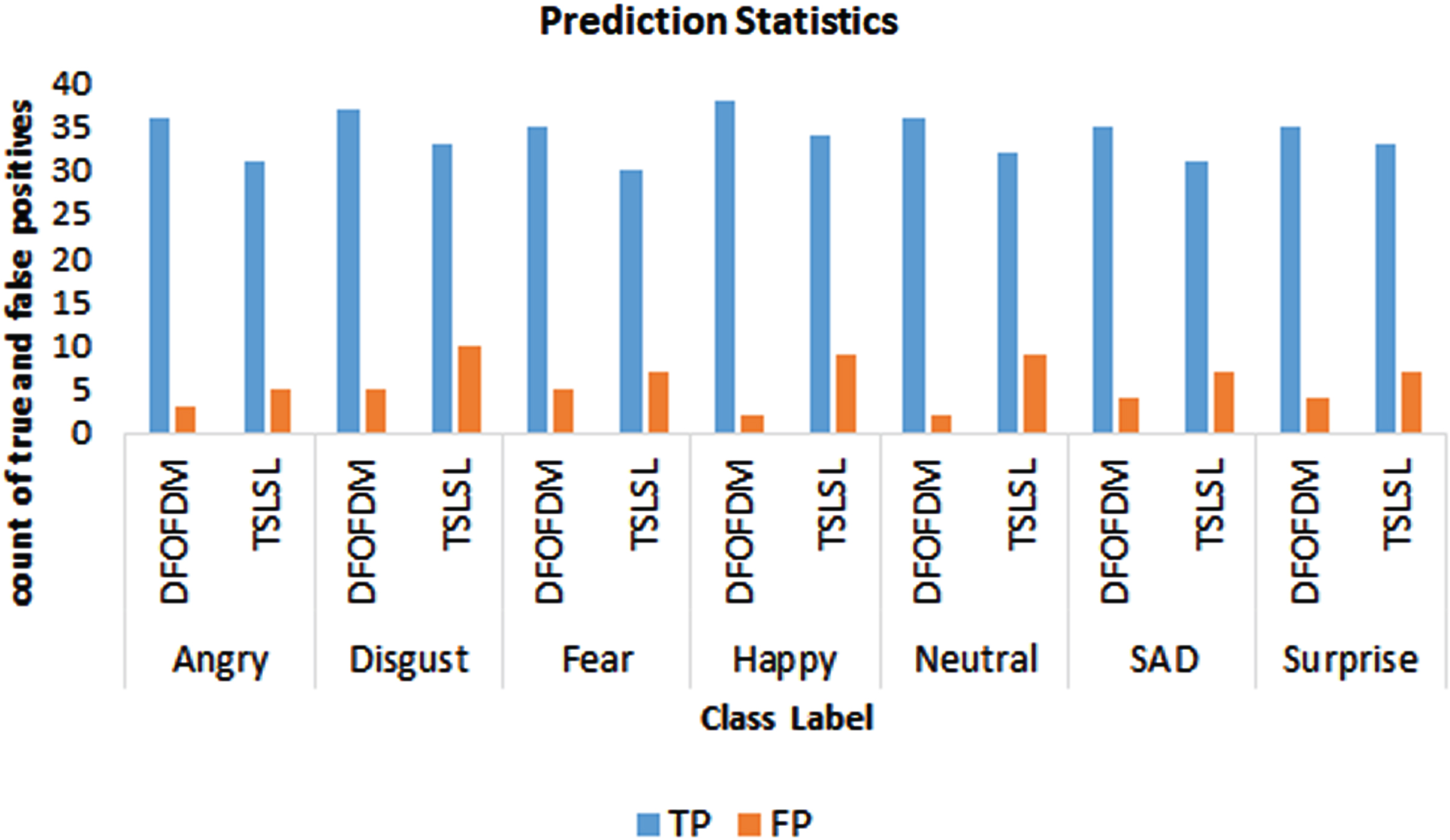
TP and FP statistics for both DFOFDM and TSLSL.

For instance, for the ‘Angry’ label, the DFOFDM model demonstrates a higher TP rate (36/40 = 90%) and a lower FP rate (5/39 =∼12.82%) as compared to the TSLSL model which has a TP rate of 31/40 = 77.5% and an FP rate of 5/36 =∼13.89%. This pattern of superior performance by DFOFDM in terms of higher TP and lower FP rates extends across all labels, indicating its overall enhanced performance in emotion recognition from speech signals.

Top of Form

The performance of the suggested model DFOFDM, as indicated by the precision, recall, and F-score metrics derived from the confusion matrix, is displayed in Table 6. The model achieved impressive true positive rates (precision) exceeding 92% for the labels “Angry”, “Happy”, and “Neutral”. For “Disgust”, “Fear”, “Sad”, and “Surprise” labels, the precision fell between a still respectable range of 87% and 90%. In terms of recall, which measures the model’s ability to identify all relevant instances, the DFOFDM exhibited values ranging from 90% to 95% for the labels “Angry”, “Disgust”, “Happy”, and “Neutral”. For the remaining labels, “Fear”, “Sad”, and “Surprise”, recall values were slightly lower, between 87% and 90%. The F-score, a metric combining precision and recall, mirrored these results, with “Angry” at 91%, “Disgust” at 90%, “Fear” at 87%, “Happy” at 95%, “Neutral” at 92%, “Sad” at 89.7%, and “Surprise” at 89.7%.

Table 6

Statistics of the independent metrics discovered from the confusion matrix of the DFOFDM

Label	TP	FP	Precision	Recall/ sensitivity/ accuracy	F-SCORE
Angry	36	3	0.9231	0.9	0.9114
Disgust	37	5	0.881	0.925	0.9025
Fear	35	5	0.875	0.875	0.875
Happy	38	2	0.95	0.95	0.95
Neutral+	36	2	0.9474	0.9	0.9231
Sad	35	4	0.8974	0.8974	0.8974
Surprise	35	4	0.8974	0.8974	0.8974

On the other hand, the performance statistics of a contemporary model, TSLSL, are presented in Table 7. This table provides “precision, recall, and F-Score” values for each label: “Angry” (86.11% precision, 77.5% recall, 81.58% F-Score), “Disgust” (76.74% precision, 82.5% recall, 79.52% F-Score), “Fear” (81.08% precision, 75% recall, 77.92% F-Score), “Happy” (79.07% precision, 85% recall, 81.93% F-Score), “Neutral” (78.05% precision, 80% recall, 79.01% F-Score), “Sad” (81.58% precision, 79.49% recall, 80.52% F-Score), and “Surprise” (82.5% precision, 84.62% recall, 83.55% F-Score). Notably, these metrics are markedly lower than those obtained with the proposed DFOFDM model, underscoring DFOFDM’s superior performance in emotion recognition from speech signals.

Table 7

Statistics of the independent metrics discovered from the confusion matrix of the TSLSL

Label	TP	FP	Precision	RC/ sensitivity/ accuracy	F-SCORE
Angry	31	5	0.8611	0.775	0.8158
Disgust	33	10	0.7674	0.825	0.7952
Fear	30	7	0.8108	0.75	0.7792
Happy	34	9	0.7907	0.85	0.8193
Neutral	32	9	0.7805	0.8	0.7901
Sad	31	7	0.8158	0.7949	0.8052
Surprise	33	7	0.825	0.8462	0.8355

Figure 4: This figure provides a visual comparison of the precision achieved by the DFOFDM and TSLSL models for different emotion labels: “Angry, Disgust, Fear, Happy, Neutral, Sad, and Surprise”. Precision is measured as the ratio of “true positives (TP)” to the sum of TP and “false positives (FP)”. Each label is associated with two bars - one for DFOFDM and the other for TSLSL.

Fig. 4

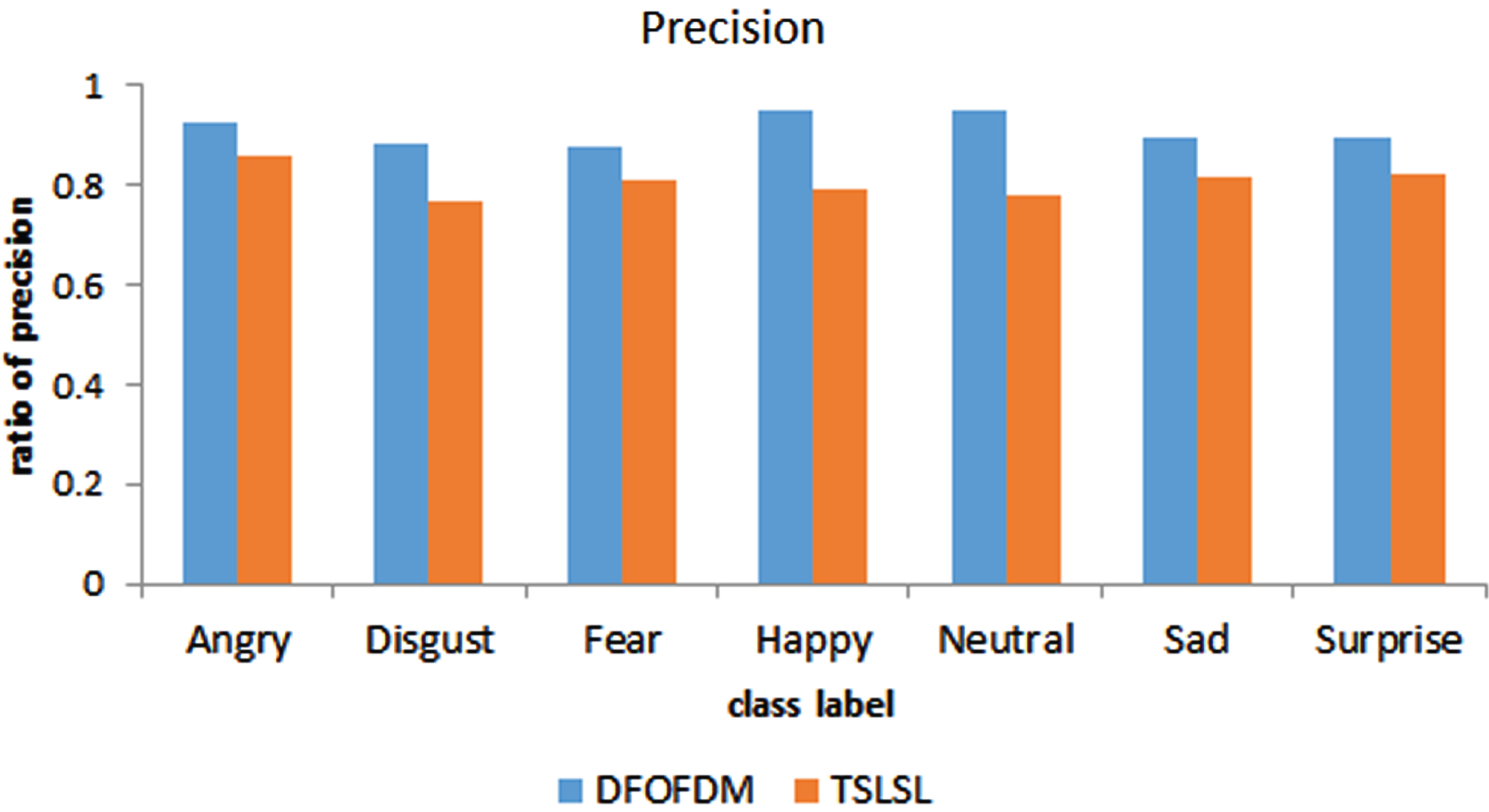
Measured precision of DFOFDM as well as TSLSL for diverse labels.

For example, for the ‘Angry’ label, DFOFDM achieves a precision rate of 36/39 =∼92.31%, outperforming the TSLSL model, which scores a precision rate of 31/36 =∼86.11%. This pattern of superior precision performance by the DFOFDM model is consistent across all emotion labels. It is evident from this figure that DFOFDM provides a more accurate classification of the different emotions compared to the TSLSL model, thereby enhancing the overall effectiveness of speech emotion recognition.

Figure 5: This figure provides a detailed comparison between the sensitivity (also known as recall) of the DFOFDM and TSLSL models across various emotion labels: “Angry, Disgust, Fear, Happy, Neutral, Sad, and Surprise”. Sensitivity is calculated as the ratio of “true positives (TP)” to the sum of true positives and “false negatives (FN)”. In this figure, each label is represented with two bars, one indicating the sensitivity of the DFOFDM model and the other showing the sensitivity of the TSLSL model.

Fig. 5

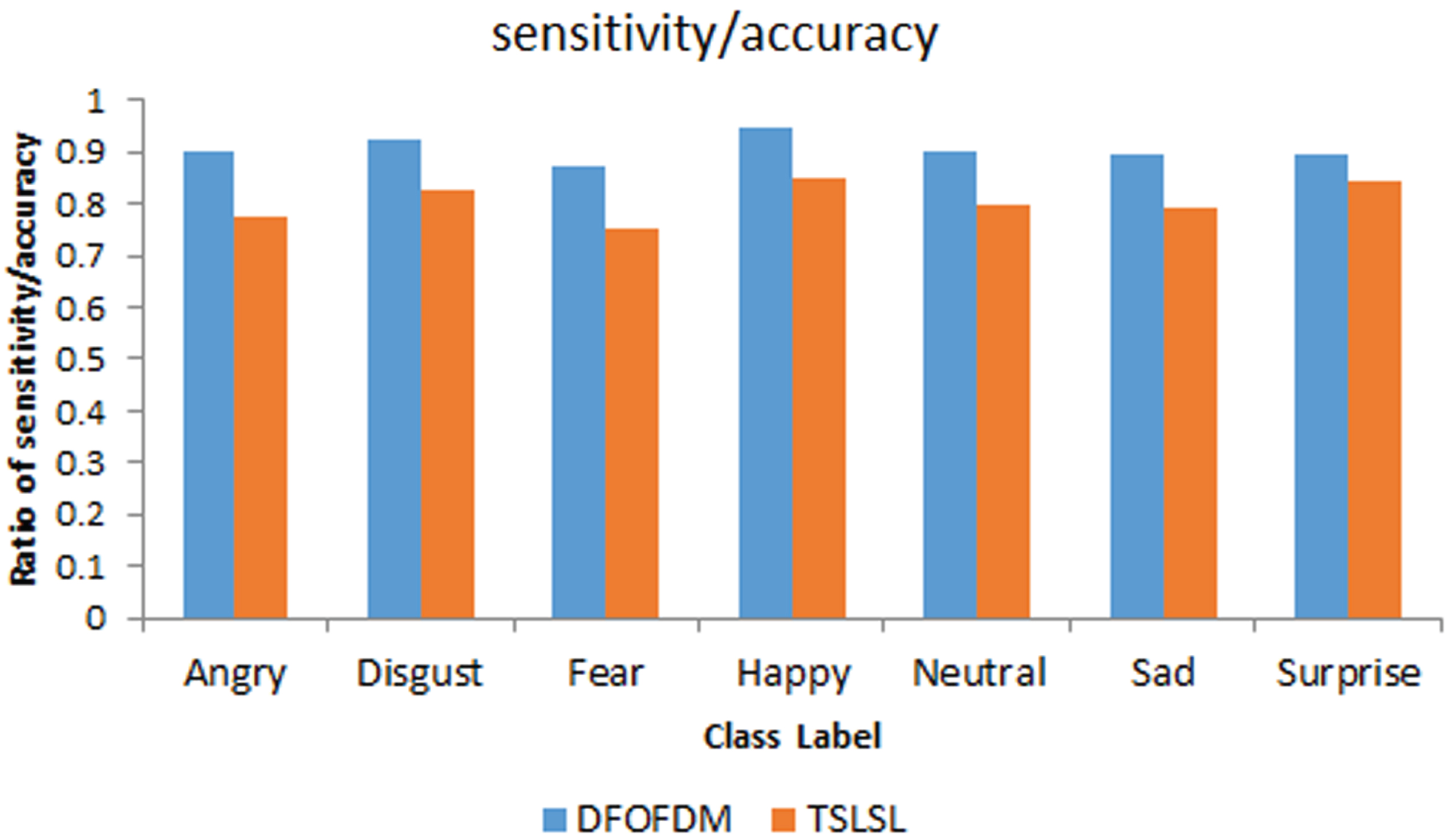
Measured sensitivity of DFOFDM as well as TSLSL for diverse labels.

For instance, for the ‘Angry’ label, DFOFDM presents a sensitivity rate of 36/40 = 90%, which is higher than the TSLSL model’s sensitivity rate of 31/40 =∼77.5%. This trend of DFOFDM outperforming the TSLSL model in terms of sensitivity is observed consistently across all emotion labels. This figure clearly demonstrates that DFOFDM is more effective in correctly identifying true instances of each emotion, thereby boosting the overall performance of the speech emotion recognition system.

Figure 6 shows a correlation between F-score and several types of emotional expression for both the proposed DFOFDM and the currently used TLSL models. The F-Score is the harmonic mean of the measures of accuracy and recall. In comparison to the current TSLSL technique, the F-Score of the proposed DFOFDM approach is higher for each category of emotions (Fig. 6).

Fig. 6

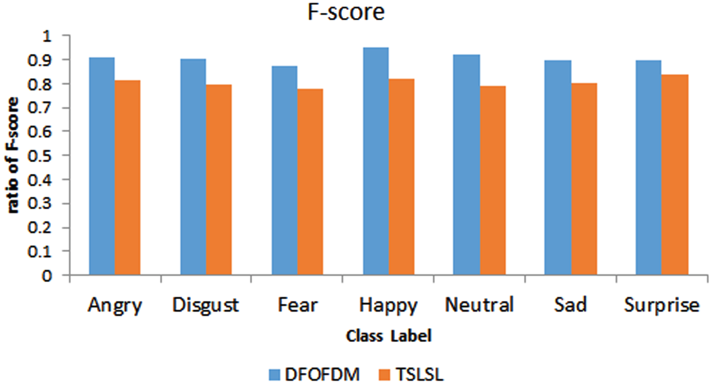
Measured F-score of DFOFDM as well as TSLSL for diverse labels.

A multi-label classifier’s total performance may be determined by calculating its “weighted-precision, weighted-recall, and weighted f-score”. Multi-label classifier labels (positively treats) do not correspond to each other (negative part). In the context of multi-label classification, these values of the metrics “PPV (positive predictive value)”, “TPR (true positive rate)”, f-score, as well as decision accuracy will allow for scaling the performance of the classifier (not the label).

Table 8 presents the statistics for dependent metrics, which are derived from the precision, sensitivity, and F-score values for each label “(Angry, Disgust, Fear, Happy, Neutral, Sad, and Surprise)” of the DFOFDM model. The “Weighted Precision, Weighted Recall, and Weighted F-Score” are evaluated for each label to give a comprehensive understanding of the model’s performance across multiple measures. The table reveals that the values are generally above 34%, demonstrating a robust performance of the DFOFDM model across different labels. The highest values are observed for the “Happy” label, suggesting optimal emotion recognition in this category.

Table 8

Statistics of the dependent metrics discovered from the precision, sensitivity, as well as f-score values of DFOFDM

Label	Angry	Disgust	Fear	Happy	Neutral	Sad	Surprise
Weighted Precision	36.924	35.24	35	38	37.896	34.9986	34.9986
Weighted Recall	36	37	35	38	36	34.9986	34.9986
Weighted F-Score	36.456	36.1	35	38	36.924	34.9986	34.9986

Table 9 displays the statistics for the dependent metrics derived from the precision, sensitivity, and F-score values for each label “(Angry, Disgust, Fear, Happy, Neutral, Sad, and Surprise)” of the TSLSL model. The “Weighted Precision, Weighted Recall, and Weighted F-Score” provide a multi-faceted understanding of the model’s performance for each emotion label. The values primarily range from the low 30% to mid-30%, indicating a decent performance by the TSLSL model across different labels. Nevertheless, these figures are slightly lower than those of the DFOFDM model (as seen in Table 8), suggesting that DFOFDM might have superior overall performance in emotion recognition from speech signals.

Table 9

Statistics of the dependent metrics discovered from the precision, sensitivity, as well as f-score values of TSLSL

Label	Angry	Disgust	Fear	Happy	Neutral	Sad	Surprise
Weighted Precision	34.444	30.696	32.432	31.628	31.22	31.8162	32.175
Weighted Recall	31	33	30	34	32	31.0011	33.0018
Weighted F-Score	32.632	31.808	31.168	32.772	31.604	31.4028	32.5845

Weighted-precision, Weighted-F-score, as well as weighted-recall data for the proposed technique DFOFDM and the Current method TSLSL are shown in Tables 8 and 9, respectively. The cross-validation statistics have been weighted based on the total input records for each of the labels and the recall, f-score, as well as accuracyobserved for that label. As the independent metrics “accuracy”, “recall”, and “f-score” have an effect on the final values of these metrics, the current model TSLSL has scaled down in comparison to the suggested model DFOFDM.

Find the micro values (classification level) recall, precision, as well as f-measure from the “weighted-precision”, “weighted-recall”, and “weighted f-score” of each emotion category. These estimates of performance parameters at the micro level shall look like this. The empirical probability of each metric (precision, recall, and f-score) was calculated by observing the ratio of the total number of test records to the sum of all labels. Table 10 shows the results of a statistical analysis of classifier performance.

Table 10

Micro-precision, micro-F-score, as well as micro-recall of the DFOFDM and TSLSL

	Micro-precision	Micro-recall	Micro F-score	Prediction Accuracy
DFOFDM	0.9103	0.9065	0.9082	0.9083
TSLSL	0.8072	0.8058	0.8057	0.8062

Table 10 presents a comparative analysis of the micro-level metrics of the two models, DFOFDM and TSLSL. The metrics include “micro-precision”, “micro-recall”, “micro F-score”, and “prediction accuracy”. These micro-level metrics offer an aggregate measure of the models’ overall performance, not segregating into different emotion labels.

For the DFOFDM model, the “micro-precision, micro-recall, micro F-score, and prediction accuracy” values are around 0.91, indicating a high level of overall precision, sensitivity, and accuracy in the emotion recognition task. These values suggest that the DFOFDM model has a strong performance in correctly predicting labels and minimizing false identifications.

In contrast, the TSLSL model demonstrates a lower overall performance, with “micro-precision, micro-recall, micro F-score, and prediction accuracy” values close to 0.81. Despite being lower than the DFOFDM model, these figures still suggest a solid performance. Nonetheless, when compared side by side, the DFOFDM model outperforms TSLSL in terms of these aggregate metrics.

The significance of the proposal DFOFDM has evinced underperformance metrics micro-precision (91.03%), micro-recall (90.65%), micro-F-score (90.82%), and decision accuracy (90.83%), which have compared to the corresponding micro-precision (80.72%), micro-recall (80.58%), as well as micro-F-score (80.57%), and decision accuracy (80.62%) of the counterpart TSLSL.

4.4 Analysis of computational complexity

This section, delves into the efficiency and scalability of our proposed method with regard to contemporary models, focusing on the “Complexity of Feature Optimization” and the “Complexity of Learning.” These in-depth analyses illuminate the computational trade-offs in feature selection, optimization, and the learning process, aiding in the method’s optimal deployment in diverse settings.

4.4.1 Complexity of feature optimization

Computational complexity refers to the computational resources needed to solve a problem. The computational complexities of Ant-Colony, GA, PSO, and NSGA II differ in nature due to their different methodologies, but they all generally have high computational complexity due to their iterative and explorative nature.

“Genetic Algorithms (GAs) [13]”: The computational complexity of GAs is usually high and it depends on the number of generations, the population size, and the length of the chromosome. This usually leads to a computational complexity of O (gnm), where g is length of a chromosome, m, and n, the total number of generations.

“Ant Colony Optimization (ACO) [13]”:The quantity of ants as well as the magnitude of the issue are the main determinants of ACO’s time complexity. The time complexity of the Travelling Salesman Problem is m (city sizes)(ant sizes) O (n² * m), where n (city sizes), O (n² * m) (city sizes) and m (ant sizes).

“Particle Swarm Optimisation (PSO) [16]” has a temporal complexity of O (n * m) for a fixed number of particles n as well as m for a fixed number of iterations. When there are extensive search areas involved or a lot of iterations are required to reach convergence, this might be high.

“NSGA II [15]”: The NSGA II’s computational complexity is primarily due to the sorting of the population into different fronts and the diversity calculation. The complexity of sorting in NSGA II is O (m * n²), where n is the size of the population and m is the number of objectives.

Fusion of the distribution diversity assessment measures: However, the combination of distribution diversity assessment tools such“Mann-Whitney U Test”, “Kolmogorov-Smirnov Test, and Dual tailed t-Test typically have much lower computational complexity. The Mann-Whitney U Test” has a time complexity of O (n log(n)) due to the need to sort the data, the Kolmogorov-Smirnov Test also has a complexity of O (n log(n)), and the t-Test has a complexity of O (n), where n is the number of data points. The fusion of these methods would likely maintain a complexity within the same order.

4.4.2 Complexity of learning

“Convolutional Neural Networks (CNNs) [20, 35]”: Complexities of computing of a CNN depends on the dimensions of the input data, the number of filters, filter dimensions, stride length, and the number of layers. Overall, the time complexity of a convolutional layer is O (nmlij), where n is the number of filters, m is the dimension of the filters, l is the dimension of the output feature maps, and i, j are the dimensions of the input.

“Support Vector Machines (SVMs) [22, 28]”: The time complexity of training an SVM is between O (n²) and O (n³), where n is the number of training examples, assuming a fixed number of features. The high computational complexity arises from the need to solve a quadratic programming problem.

“Deep Convolutional Neural Networks (DCNNs) [35]” with a rectangular kernel: Similar to a regular CNN, the computational complexity of a DCNN depends on various factors. However, as the network gets deeper, the complexity grows. The complexity of a convolutional layer with a rectangular kernel is also O (nmlij), with the same variable assignments as a CNN, but each variable could be significantly larger due to the depth and kernel shape.

Ensemble Softmax regression model [25]: The complexity of an Ensemble Softmax regression model is primarily influenced by the number of classifiers in the ensemble and the complexity of each classifier. If we assume that the complexity of each individual softmax regression is O (nm), When m is the number of classes and n is the number of features, the complexity for k classifiers would be O (kn * m).

Transfer linear subspace learning [37]: The computational complexity of Transfer linear subspace learning largely depends on the size and architecture of the pre-trained model, and the size of the new dataset. When the pre-trained model is large (e.g., a deep learning model like BERT or ResNet), the computational cost of training could be high. However, as these models are often fine-tuned, meaning only the final layers are updated while earlier layers are frozen, the computational cost is less than training the model from scratch.

“Cuckoo Search (CS)”: The computational complexity of CS is typically O (t * n), where t is the number of iterations or generations and n is the population size (number of solutions). However, this can increase depending on the complexity of the fitness function. The complexity of the fitness function derived in the proposed DFOFDM is O (L * nG * H * l), which is relatively low. Hence the overall computational complexity of DFOFDM is relatively low that compared to contemporary models.

5 Conclusion

In conclusion, the article has presented a detailed study on “Emotion Recognition from Speech Signals Using Digital Features Optimization by Diversity Measure Fusion” (DFOFDM), comparing its performance with a contemporary model known as TSLSL. Through rigorous testing and statistical analysis, the study finds that the DFOFDM model outperforms TSLSL in several key metrics such as precision, recall, and F-score, across diverse emotion labels, demonstrating its potential for practical applications in the area of emotion recognition. The DFOFDM model exhibited superior performance, yielding higher values for “precision, recall, and F-score”, across all the seven emotion labels considered: “angry, disgust, fear, happy, neutral, sad, and surprise”. Micro-level metrics, including “micro-precision, micro-recall, micro F-score, and prediction accuracy”, were also found to be superior in the DFOFDM model. This is a testament to the strength of the DFOFDM approach in managing the multi-label classification task, particularly in the challenging domain of emotion recognition from speech signals. However, this study does not suggest that the DFOFDM is a flawless model. While it shows promise, it also exhibits certain limitations that should be acknowledged. For instance, DFOFDM’s performance is highly dependent on the quality and variability of the speech signals used. Poor quality speech data or data with low variability can limit the model’s ability to discern between different emotional states accurately. Furthermore, the performance of DFOFDM can be influenced by the language and the cultural background of the speakers in the dataset, as well as by the speaker’s individual traits, such as their speech patterns and emotional expressivity. Therefore, the model might need to be fine-tuned and adapted for different languages, cultures, and individual traits to ensure robust and universal applicability. Looking ahead, future research should consider exploring these limitations and working towards their solutions. It would be beneficial to extend the application of the DFOFDM model to more diverse datasets, encompassing a variety of languages, cultures, and individual traits. Additionally, future studies could investigate ways to improve the model’s robustness to noise and variability in speech signals. Moreover, as technology continues to evolve, there will be opportunities to integrate the DFOFDM model with other emerging technologies such as deep learning and artificial intelligence. The fusion of these technologies could lead to further advancements in emotion recognition systems, making them even more accurate, reliable, and adaptable to real-world applications.