Sage Journals: Discover world-class research

Abstract

The Spiral Drawing Test (SDT) has become a prominent clinical marker for the early diagnosis of Parkinson’s Disorder (PD) by capturing tremor symptoms. The integration of AI algorithms into a PD diagnosis system has proven to be a breakthrough objective assessment that aids professionals in decision-making. However, there is a need for improvisation of the workflow architectures of AI models to optimize the diagnosis system by reducing the misdiagnosis rate. The proposed system presents PD prediction using a Spiral Drawing Test (SDT) image modality integrated with an Artificial Intelligence (AI) algorithm. The proposed study presents three hybrid workflow architectures formed by integrating three core layers: a data augmentation layer, Transfer Layer (TL)-based feature extraction layer, and Deep Learning (DL)-based classification layer. The results were analyzed by conducting 18 experiments based on the hyperparameter values and workflow architectures. The highest accuracy obtained by the proposed study is 98% for Hybrid Workflow Architecture II.

Keywords

Parkinson disorder transfer learning

1 Introduction

Problem Domain Definition: Parkinson Disorder (PD) is a neurological condition in which PD patients experience motor and non-motor symptoms. PD diagnosis at an early stage is vital to avoid the progression of the disorder. The most prominent motor manifestations are dysphonia, tremor, rigidity and slowness of movement known as bradykinesia. The non-motor manifestations are sleep problems and psychiatric problems mainly depression and bipolar disorder. PD affects largely the individuals above the age of 65.

1.1 Identification of problems

The problems identified in PD diagnosis system are:

There is no PD specific diagnosis system mapped with its stages.

Negligence of early symptoms of PD in the diagnosis phases.

Non usage of cost effective and noninvasive methods for PD diagnosis.

Subjective assessment is higher compared to objective assessment.

1.2 Possible solutions

The possible solutions to combat the identified problems are:

Development of non-invasive PD diagnosis system which is cost-effective and mapping the early symptoms of PD.

Amalgamation of AI to the non-invasive modalities for objective assessment based effective decision making in PD diagnosis which aids clinicians to make diagnosis in an efficient manner.

1.3 Motivation

The prevalence rate of Parkinson Disorder (PD) worldwide is 7-10 million approximately [1]. The early symptoms namely dysphonia and tremor if captured and diagnosed with the integration of non-invasive modalities, there is high possibility for delaying the progression of disorder.

Artificial Intelligence is the tremendously growing technology which is useful for many applications that covers high scale systems, middle scale systems and large scale systems. Machine Learning (ML) is the branch of AI and Deep Learning (DL) is the extended version of Artificial Neuron Network (ANN), a ML model. Transfer Learning (TL) is the advanced version of DL models which uses pre-trained models and transfers the model learning from one application to another specific application. AI algorithms are widely used in medical applications by integrating to the non-invasive modality [2].

The list of abbreviations used in this paper is specified in Table 1.

Table 1
List of Abbreviations

SI.No Acronyms Abbreviations

1 PD Parkinson Disorder

2 HS Healthy Subject

3 SDT Spiral Drawing Test

4 AI Artificial Intelligence

5 TL Transfer Learning

6 LR Logistic Regression

7 RFC Random Forest Classifier

8 CNN Convolutional Neural Network

9 ROC Receiver Operating Characteristics

10 ML Machine Learning

11 KNN K Nearest Neighbor

12 SVC Support Vector Classification

13 CC-Net Continuous Convolutional Neural Network

14 DL Deep Learning

15 LMC Leap Motion Controller

16 ResNet Residual Network

17 AdaBoost Adaptive Boosting

18 SVM Support Vector Machine

19 LSTM Long Short-Term Memory

20 DenseNet Deep Convolutional Network

21 HWA-I Hybrid Workflow Architecture-I

22 HWA-II Hybrid Workflow Architecture-II

23 HWA-III Hybrid Workflow Architecture-III

SI.No	Acronyms	Abbreviations
1	PD	Parkinson Disorder
2	HS	Healthy Subject
3	SDT	Spiral Drawing Test
4	AI	Artificial Intelligence
5	TL	Transfer Learning
6	LR	Logistic Regression
7	RFC	Random Forest Classifier
8	CNN	Convolutional Neural Network
9	ROC	Receiver Operating Characteristics
10	ML	Machine Learning
11	KNN	K Nearest Neighbor
12	SVC	Support Vector Classification
13	CC-Net	Continuous Convolutional Neural Network
14	DL	Deep Learning
15	LMC	Leap Motion Controller
16	ResNet	Residual Network
17	AdaBoost	Adaptive Boosting
18	SVM	Support Vector Machine
19	LSTM	Long Short-Term Memory
20	DenseNet	Deep Convolutional Network
21	HWA-I	Hybrid Workflow Architecture-I
22	HWA-II	Hybrid Workflow Architecture-II
23	HWA-III	Hybrid Workflow Architecture-III

1.4 Organization of the paper

The remaining of the paper is organized as follows –section 2 discusses the related works which focuses on presenting the methods, pros and cons of the existing system, section 3 presents the research methodologies which focuses on the detailed explanation of all the components present in the proposed workflow architectures, section 4 presents the results analysis which provides the insights and inferences acquired from analyzing and interpreting the results and section 5 concludes the paper.

1.5 Contributions of the paper

Architecture: The design and implementation of three hybrid workflow architectures formed by amalgamation of three core layers: data augmentation layer, Transfer Learning (TL) based feature extraction layer and Deep Learning (DL) based classification layer.

Customized Classification Layer: The novel classification layer is designed separately and the fully connected classification layer of pre-trained model is not used.

Hyperparameter Based Experiments: The conduction of experiments is based on hyperparameters and total number of experiments conducted are 18.

2 Related works

The related works is presented in two main categories:

1) Survey based on PD diagnosis using Handwritten and Sketch Drawings Image Modality

2) Survey based on Different Deep Learning and Transfer Learning Methods

2.1 Survey based on PD diagnosis using hand-written and sketch drawings image modality

Sabyasachi Chakraborty et al [2], presents a multistage classifier network architecture for the diagnosis of Parkinson Disorder (PD) based on spiral and wave drawings image dataset. The multistage classifier consists of two convolutional networks for generation of probabilities and prediction based on spiral and wave drawings respectively and it also consists of two meta classifiers namely Logistic Regression (LR) and Random Forest Classifier (RFC) which is an ensemble that combines the probabilities generated by two convolutional networks and provides the final prediction. The advantage of the multistage classifier is that the ensemble layer paves ways for integrated analysis of two Convolutional Neural Network (CNN) which provides robustness in prediction. The disadvantage of the system is that the data size is of less amount to train deep learning models and to arrive at conclusions. The accuracy obtained for the multistage classifier is 93.3%. Marta San Luciano et al [3] provides a digitized spiral drawing data acquisition and statistical analysis of the procured data. The methods used for data acquisition are generation of coordinates corresponding to pressure, the derivation of indices corresponding to kinematics of data and Receiver Operating Characteristic (ROC) analysis. The advantage of the study is that it provides a strong proof of the impact of derivation of indices from digitized spiral images in differentiation of PD from healthy subjects. The disadvantage of the study is that it does not provide proof that digitized spiral drawing data modality is effective biomarker specialized for PD diagnosis. Megha Kamble et al [4] contributes a spiral drawing image modality-based PD prediction by combining the feature engineering technique and Machine Learning (ML) algorithm. The feature engineering technique focuses on generation of kinematic features and spatiotemporal features from the digitized spiral drawing images. The ML algorithms considered are K Nearest Neighbor (KNN), Logistic Regression, Random Forest Classifier (RFC) and Support Vector Classifier (SVC). The advantage of the system is the generation of new kinematic features in the feature engineering process. The disadvantage of the system is that the data is in imbalanced form. The procured accuracy of the system is 91.6%. Sarah Fan et al [5] presents a Convolutional Neural Network (CNN) for early diagnosis of Parkinson Disorder (PD) based on spiral drawings, wave drawings and meander drawings dataset. The CNN model consists of five layers namely convolutional layers, pooling layers, drop out layers, dense layers and flattened layers with each layer consisting of two sub layers. The study confirms from the results that spiral drawings-based CNN model outperforms other drawings dataset CNN for proper discrimination of PD subject from healthy subject. The advantage of the study is that the finding of best modality for PD prediction by comparing with all combinations of data modalities. The disadvantage of the system is the lack of exploration in Transfer Learning (TL) models and multi stage CNN models. Manuel Gil-Martín et al [6] provides a PD diagnosis system by integrating CNN model to the digitized spiral drawings dataset. The CNN model consists of the feature extraction part wherein convolutional layers are incorporated and classification part wherein fully connected layers are incorporated. The CNN model provides an accuracy of 96.5%. The advantage of the system is the inclusion of Fourier transform spectrum as input to the CNN model for better prediction. The disadvantage of the system is the lack of augmentation in data to increase data size and data dynamics. Continuous Convolutional Neural Network (CC-Net) is proposed and implemented in paper [7] which performs classification of PD and healthy subjects based on spiral drawings images. The advantage of the system is the use of fewer pooling layers in order to maintain the quality of the extracted features as more pooling layers may lead to change of important features in the image data. The disadvantage of the system is that the accuracy obtained by the system is 89.3%, further optimization of hyperparameters and architecture is essential to improve the performance of the system. Elli Valla et al [8] presents the PD diagnosis system by providing novel features based on tremor and also by incorporation of feature selection techniques and ensemble-based classifiers for classification of PD patients and healthy subjects. The advantage of the system is that extraction of tremor related features for classification as it acts as a clear indicator. The disadvantage of the system is the small sample size as Machine Learning and Deep Learning (DL) models require large samples with variations for proper classification. Iqra Kamran et al [9] presents the deep Transfer Learning (TL) models for PD assessment based on handwritten data images. The advantage of the system is the incorporation of augmentation techniques to increase the sample size which eventually aids in improving the performance of the model, thereby allowing the system to produce an accuracy of 99.22%. The future scope of the system is the procurement of complex task dataset integrated with appropriate clinical features which provides diversity in data and helps in enhancement of the model learning and performance. C. Kotsavasiloglou et al [10] presents a Machine Learning (ML) model for prediction of PD based on simple line drawings. The system obtained an accuracy of 91%. The advantage of the system is the experimental set up designed properly with appropriate measurements and protocols. The limitation of the system is that it lacks simple line drawings data with respect to non-PD subjects who have tremor issues which helps to draw conclusions that the simple line drawings image modality is a specific diagnostic marker for PD. Moises Diaz et al [11] presents a PD diagnosis system based on handwritten images modality and a Transfer Learning (TL) model for efficiency feature extraction integrated with the Convolutional Neural Network (CNN) framework for initial prediction. The final prediction is provided by the ensemble classifiers. The advantage of the system is the use of TL model for feature extraction as it is computationally efficient, thereby reducing the time complexity. The disadvantage of the system is the lack of inclusion of ensemble selection mechanism which allows the classifiers to be included for final prediction, as it plays a major role in the authenticity of the overall accuracy of the system. Shoujiang Xu et al [12] presents an ensemble method for PD prediction based on the handwritten image’s dataset. The ensemble architecture is formed based on the fusion of six Random Forest (RF) classifiers and Principal Component Analysis (PCA). The advantage of the system is the incorporation of RF classifiers to the ensemble as it is easy to implement and has fewer parameters. The spatial parameters are only focused in the study which is considered to be the limitation which can be solved by combining spatial and temporal parameters. Machine Learning (ML) methods are incorporated in paper [13] for classification of Healthy Subjects (HS) and Parkinson Disorder (PD) subjects based on pressure features. The ML methods which are incorporated are Adaptive Boosting (AdaBoost) classifier, K Nearest Neighbor (KNN) and Support Vector Machines (SVM). The advantage of the system is the handwriting analysis with eight different tasks which provides robustness in the system for arriving at conclusions appropriate to PD diagnosis. The future focus of the system is the use of the standardized data collection protocols with different scenarios and variations. A novel method is proposed in paper [14] based on the motion points derived from Leap Motion Controller (LMC) is used for differentiation of tremors among Parkinson Disorder (PD) patients and other disorders. The Convolutional Neural Network (CNN) - Long Short-Term Memory (LSTM) is used as the prediction model. The advantage of the system is the novel incorporation of tremor differentiation based on LMC for diagnosis which aids clinicians from not making misdiagnosis decisions. The future scope of the system is the incorporation of a monitoring or tracking system regularly for patients, thereby providing a telemonitoring system which helps the patients and the clinicians. C.D. Rios-Urrego et al [15] presents the handwriting analysis and evaluation system based on features namely geometrical features, kinematic features and non-linear features for PD diagnosis. The advantage of the system is the integration of three features which helps in effective PD prediction. The future focus of the system is to perform the longitudinal study implementation. The short summary of the survey based on PD diagnosis system using Handwriting and Sketch Drawings Image Modalities are:

The highest accuracy (99.9%) is obtained in the research conducted by Elli Valla et al, however ensemble-based feature selection technique is used for accurate prediction, the sample size is small and hybrid based augmentation is not employed for incrementing sample size as higher sample size is crucial for ML and DL models to provide reliable prediction.

It is inferred from the results of the research in the literature that the transfer learning, deep learning models provide higher accuracy for PD prediction compared to Machine Learning (ML) models for image based modality.

2.2 Survey based on different deep learning and transfer learning methods

Gao Huang et al [16] presents Transfer Learning methods namely DenseNets abbreviated as Deep Convolutional Network with four versions. The four versions of DenseNets are DenseNet-121, DenseNet-169, DenseNet-201 and DenseNet-264. The main principle behind the working of DenseNet is that there is a feed forward manner connection between each layer to all other layers. The advantages of DenseNet architecture are the reduction of the problem of vanishing gradient, enhances the feature propagation by strengthening, it has reduced the number of parameters and allows for reuse of features. The matching of feature sizes is performed by Dense-Net, a densely connected convolutional network architecture for providing maximum information flow between the layers of the network by direct connection. Kaiming He et al [17] presents the ResNet abbreviated as Residual Nets. The prominent versions of ResNets are ResNet -20, ResNet -32, ResNet -44, ResNet-110 and ResNet -1202.The advantage of using ResNets is that the training becomes easier and it solves the problem of degradation in an efficient way by using the residual frameworks mapping rather than using unreferenced mapping. Olaf Ronneberger et al [18] presents a U-Net Transfer learning method which consists of two paths namely the contracting path and the expansive path. The contracting path is responsible for down sampling and the expansive path is responsible for up sampling. The contracting path which down samples leads to doubling the feature channels and the expansive path which up-samples results to the outcome that halves the feature channels. The main application of U-Net is segmentation of biomedical images. Mingxing Tan et al [19] presents a TL method based on Convolutional Neural Network (CNN) namely EfficientNet. The main methodology behind the EfficientNet model is to scale up the CNN models by using the compound coefficient. The advantage of the EfficientNet model is the improvement in model performance significantly by scaling through a balanced network which consists of balanced width, depth and resolution. Andrew Howard et al [20] presents a MobileNet V3 model of two versions namely MobileNetV3 - Large and MobileNetV3 - Small which is useful for mobile devices-based computer vision applications. The MobileNetV3 architecture leverages network search and design techniques.

The short summary of the survey based on different Deep Learning (DL) and Transfer Learning (TL) models:

DenseNet are efficient method for feature extraction process for image-based modality.

ResNet models computationally feasible as it makes the training process easier.

U-Net models plays a prominent in segmentation process of images.

EfficientNet model is used for scaling CNN and it is efficient at improving the performance.

MobileNet V3 model is mainly used for mobile devices-based applications.

2.3 Research gaps

From the literature survey, the following research gaps related to Artificial Intelligence (AI) based PD diagnosis system has been identified and presented in Table 2. The Artificial Intelligence (AI) models used in the PD diagnosis system uses only default models which is not specific to PD SDT data. The methodological research gap present in the PD diagnosis system is that there is lack of use of hybrid data augmentation technique which is prominent to increase the SDT image data size without losing quality. The existing system didn’t use large data or if large data is incorporated, the data is not increased based on novel hybrid data augmentation techniques. The empirical research gap present in the PD diagnosis system there is lack of combinations or lack of experiments conducted in the existing to test the methods used in PD diagnosis system. The practical knowledge research gap present in the PD diagnosis system is that there is lack of exploration of hyperparameters of AI algorithms.

Table 2 presents the detailed summary of the literature survey and Table 3 presents the research gaps.

Table 2
Summary of the Literature Survey

Authors,Years Origin of Study Samples Information Methods Conclusions

Sabyasachi Chakraborty et al [1], 2020 South Korea Repository: Kaggle Data: Spiral Drawings, Wave Drawings,Total Subjects: 55, Healthy Subjects: 28, PD Subjects: 27 Muti-Stage Classifier: Two Convolutional Neural Networks (CNN) + Two Meta Classifiers (Logistic Regression, Random Forest) + Average Voting Accuracy: 93.3%

Marta San Luciano et al [2], 2016 United States (US) Data: Digitized Spiral Drawings Subjects: 288, Healthy Subjects: 150, PD Subjects: 138 Linear Mixed Effect Adjusted Models Sensitivity: 0.86, Specificity:0.81

Megha Kamble et al [3], 2021 India Repository: UCI, Data: Spiral Drawings, Subjects: 40, Healthy Subjects: 15, PD Subjects: 25 Logistic Regression, Random Forest Classifier, Support Vector Classifier, K Nearest Neighbor (KNN) Accuracy: 91.6%

Sarah Fan et al [4], 2022 United States (US) Repository: HandPD, Kaggle Data: Spiral, Meander, Wave, Subjects for HandPD data: 92 (18: Healthy, 74: PD Subjects), Subjects for Kaggle data:72 (36: Healthy, 36: PD Subjects) Convolutional Neural Network (CNN)- 2 Convolutional Layers + 2 Max - Pooling Layers, 2 Dropout Layers, 2 Dense Layers Accuracy:85%

Sarah Fan et al [4], 2022 United States (US) Repository: HandPD, Kaggle Data: Spiral, Meander, Wave, Subjects for HandPD data: 92 (18: Healthy, 74: PD Subjects), Subjects for Kaggle data:72 (36: Healthy, 36: PD Subjects) Convolutional Neural Network (CNN)- 2 Convolutional Layers + 2 Max - Pooling Layers, 2 Dropout Layers, 2 Dense Layers Accuracy:85%

Manuel Gil-Martín et al [5] Spain Data: Digitized Spiral Drawings Subjects: 77, Healthy Subjects: 15, PD Subjects: 62 Convolutional Neural Network: Convolutional Layers + Max Pooling Layers for feature extraction + Fully Connected Layer for classification Accuracy:96.5%

Zhu Li [6] China Repository: HandPD, Data: Spiral, Subjects: 126, Healthy Subjects: 43, PD Subjects: 43 Continuous Convolutional Network (CC-Net) Accuracy:89.3%

Elli Valla et al [7] Estonia Repository: DraWritePD, PaHaW Data: Spiral Drawings, Subjects: 75, Healthy Subjects: 38, PD Subjects: 37 Adaboost Decision Tree, K Nearest Neighbor (KNN), Logistic Regression, Ran-dom Forest and Support Vector Machine (SVM) Accuracy:84.33%

Ira Kamran et al [8] Saudi Arabia Repository: PaHaW + HandPD + NewHandPD + Parkinson’s Drawings, Data: Spiral, Circle, Meander, Wave, Subjects: 1534, Healthy Subjects: 561, PD Subjects: 973 AlexNet, GoogleNet, VGG 16, VGG 19, Res-Net50, ResNet 101 Accuracy:99.22%

C.Kotsavasiloglou et al [9] Greece Data: Lines Subjects: 44, Healthy Subjects: 20, PD Subjects: 24 AdaBoost, Logistic Regression, Naive Bayes and Support Vector Machine (SVM) Accuracy:90.90%

Moises Diaz et al [10] Spain Repository: PaHaW Data: Spiral Drawings, Subjects: 72, Healthy Subjects: 36, PD Subjects: 36 Two Convolutional Neural Network for combining feature vectors + two classifiers (Support Vector Machine-SVM, Random Forest - RF) Accuracy: 86.67%

Shoujiang Xu et al [11] China Repository: NewHandPD Data: Circle, Meanders, Subjects: 66, Healthy Subjects: 35, PD Subjects: 31 Random Forest Classifier + Voting Accuracy:89.4%

Peter Drotár [12] Czech Republic Data: Handwriting Tasks Images Subjects: 75, Healthy Subjects: 37, PD Subjects: 38 Adaptive Boosting Classifier (AdaBoost), K- Nearest Neighbor (KNN) and Support Vector Machine (SVM) Accuracy: 81.3%

Ayse Betul Oktay [13] Turkey Data: Track Coordinates - Leap Motion Controller (LMC), Subjects: 40, PD Subjects: 23, Other Patient subjects: 17 Convolutional Long Short-Term Memory (LSTM) Accuracy:90%

C.D. Rios-Urrego [14] Colombia Data: Spiral Drawings Subjects: 130, Healthy Subjects: 85, PD Subjects: 45 Support Vector Ma-chine (SVM), K Nearest Neighbor (KNN) and Random Forest Accuracy:93.1%

Authors,Years	Origin of Study	Samples Information	Methods	Conclusions
Sabyasachi Chakraborty et al [1], 2020	South Korea	Repository: Kaggle Data: Spiral Drawings, Wave Drawings,Total Subjects: 55, Healthy Subjects: 28, PD Subjects: 27	Muti-Stage Classifier: Two Convolutional Neural Networks (CNN) + Two Meta Classifiers (Logistic Regression, Random Forest) + Average Voting	Accuracy: 93.3%
Marta San Luciano et al [2], 2016	United States (US)	Data: Digitized Spiral Drawings Subjects: 288, Healthy Subjects: 150, PD Subjects: 138	Linear Mixed Effect Adjusted Models	Sensitivity: 0.86, Specificity:0.81
Megha Kamble et al [3], 2021	India	Repository: UCI, Data: Spiral Drawings, Subjects: 40, Healthy Subjects: 15, PD Subjects: 25	Logistic Regression, Random Forest Classifier, Support Vector Classifier, K Nearest Neighbor (KNN)	Accuracy: 91.6%
Sarah Fan et al [4], 2022	United States (US)	Repository: HandPD, Kaggle Data: Spiral, Meander, Wave, Subjects for HandPD data: 92 (18: Healthy, 74: PD Subjects), Subjects for Kaggle data:72 (36: Healthy, 36: PD Subjects)	Convolutional Neural Network (CNN)- 2 Convolutional Layers + 2 Max - Pooling Layers, 2 Dropout Layers, 2 Dense Layers	Accuracy:85%
Sarah Fan et al [4], 2022	United States (US)	Repository: HandPD, Kaggle Data: Spiral, Meander, Wave, Subjects for HandPD data: 92 (18: Healthy, 74: PD Subjects), Subjects for Kaggle data:72 (36: Healthy, 36: PD Subjects)	Convolutional Neural Network (CNN)- 2 Convolutional Layers + 2 Max - Pooling Layers, 2 Dropout Layers, 2 Dense Layers	Accuracy:85%
Manuel Gil-Martín et al [5]	Spain	Data: Digitized Spiral Drawings Subjects: 77, Healthy Subjects: 15, PD Subjects: 62	Convolutional Neural Network: Convolutional Layers + Max Pooling Layers for feature extraction + Fully Connected Layer for classification	Accuracy:96.5%
Zhu Li [6]	China	Repository: HandPD, Data: Spiral, Subjects: 126, Healthy Subjects: 43, PD Subjects: 43	Continuous Convolutional Network (CC-Net)	Accuracy:89.3%
Elli Valla et al [7]	Estonia	Repository: DraWritePD, PaHaW Data: Spiral Drawings, Subjects: 75, Healthy Subjects: 38, PD Subjects: 37	Adaboost Decision Tree, K Nearest Neighbor (KNN), Logistic Regression, Ran-dom Forest and Support Vector Machine (SVM)	Accuracy:84.33%
Ira Kamran et al [8]	Saudi Arabia	Repository: PaHaW + HandPD + NewHandPD + Parkinson’s Drawings, Data: Spiral, Circle, Meander, Wave, Subjects: 1534, Healthy Subjects: 561, PD Subjects: 973	AlexNet, GoogleNet, VGG 16, VGG 19, Res-Net50, ResNet 101	Accuracy:99.22%
C.Kotsavasiloglou et al [9]	Greece	Data: Lines Subjects: 44, Healthy Subjects: 20, PD Subjects: 24	AdaBoost, Logistic Regression, Naive Bayes and Support Vector Machine (SVM)	Accuracy:90.90%
Moises Diaz et al [10]	Spain	Repository: PaHaW Data: Spiral Drawings, Subjects: 72, Healthy Subjects: 36, PD Subjects: 36	Two Convolutional Neural Network for combining feature vectors + two classifiers (Support Vector Machine-SVM, Random Forest - RF)	Accuracy: 86.67%
Shoujiang Xu et al [11]	China	Repository: NewHandPD Data: Circle, Meanders, Subjects: 66, Healthy Subjects: 35, PD Subjects: 31	Random Forest Classifier + Voting	Accuracy:89.4%
Peter Drotár [12]	Czech Republic	Data: Handwriting Tasks Images Subjects: 75, Healthy Subjects: 37, PD Subjects: 38	Adaptive Boosting Classifier (AdaBoost), K- Nearest Neighbor (KNN) and Support Vector Machine (SVM)	Accuracy: 81.3%
Ayse Betul Oktay [13]	Turkey	Data: Track Coordinates - Leap Motion Controller (LMC), Subjects: 40, PD Subjects: 23, Other Patient subjects: 17	Convolutional Long Short-Term Memory (LSTM)	Accuracy:90%
C.D. Rios-Urrego [14]	Colombia	Data: Spiral Drawings Subjects: 130, Healthy Subjects: 85, PD Subjects: 45	Support Vector Ma-chine (SVM), K Nearest Neighbor (KNN) and Random Forest	Accuracy:93.1%

Table 3

Research Gaps

RESEARCH GAP CHARACTERISTICS	RESEARCH GAPS IDENTIFIED
Methodological Research Gap	There is a lack of hybrid data augmentation design and implementation in recent studies. There is a presence of standard data augmentation design and implementation by the existing system rather than hybrid data augmentation.
Empirical Research Gap	The experiments conducted by the existing systems from which results are procured, shows that there is a lack of different combinations of experimental parameters. (Examples: epochs and batch size with respect to the Deep Learning (DL) algorithms).
Practical Knowledge - Research Gap	The field of architecture’s hyperparameters and data augmentation parameters are less focused or explored. There are very few studies which focus on hyperparameters tuning and conduction of experiments for hyperparameters tuning.

3 Research methodologies

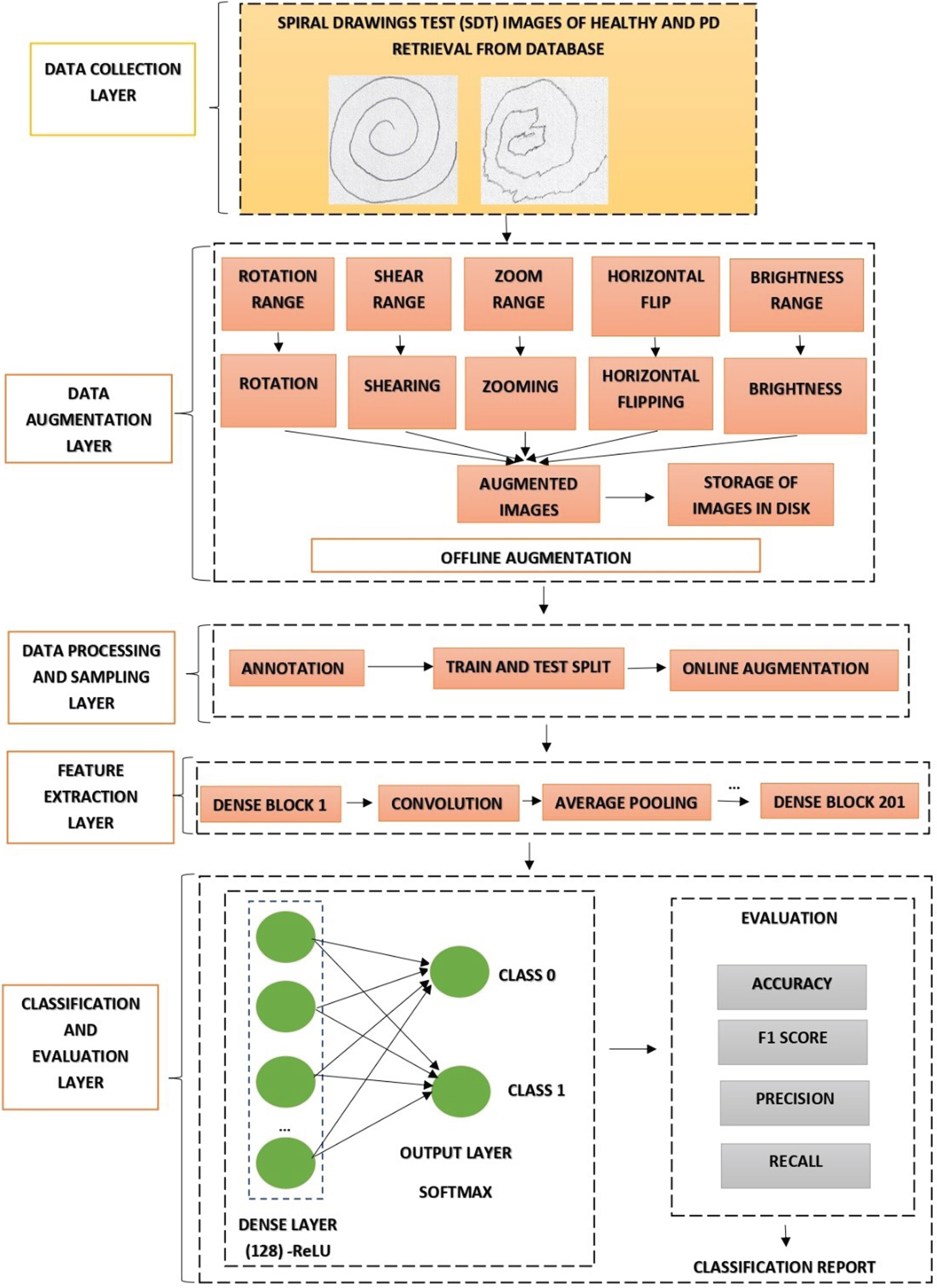
The proposed work presents three workflow architectures which is constructed by modifying with different combinations of three important aspects namely online data augmentation, offline data augmentation, hybrid data augmentation (offline + online) integrated with prominent layers. The integrated prominent layers are feature extraction layer, classification and evaluation layer. Figure 2 presents the hybrid data augmentation (offline +online). In Hybrid Workflow Architecture -I, the workflow architecture -I is constructed under five prominent layers. The five prominent layers are data collection layer, data processing and sampling layer with online augmentation, feature ex-traction layer classification and evaluation layer. In Hybrid Workflow Architecture –II the workflow architecture -II is constructed under five prominent layers. The five prominent layers are data collection layer, data augmentation layer, data processing and sampling layer without online augmentation, feature extraction layer, classification and evaluation layer. In Hybrid Workflow Architecture –III, the workflow Architecture -III is constructed under five prominent layers. The five prominent layers are data collection layer, data augmentation layer, data processing and sampling layer with online data augmentation layer, feature extraction layer, classification and evaluation layer. The novelty is presented in the data augmentation layer, it integrates offline and online data augmentation producing a hybrid data augmentation process.

3.1 Data collection layer

The Spiral Drawing Test (SDT) image dataset is retrieved from the Kaggle repository [20]. The total number of image samples present in the retrieved dataset is 102.The retrieved dataset consists of two main directories namely training and testing. The training directory consists of two sub-directories namely healthy and Parkinson. The testing directory consists of two sub-directories namely healthy and Parkinson. Table 4 presents the factual details of the samples present in the data. Figure 1 present the sample image from the dataset of one healthy and one Parkinson subject.

Table 4
Number of Samples

Directory Sub directory Number of Images Samples Total Samples

Training Healthy 36 72

Parkinson 36

Testing Healthy 15 30

Parkinson 15

Directory	Sub directory	Number of Images Samples	Total Samples
Training	Healthy	36	72
	Parkinson	36
Testing	Healthy	15	30
	Parkinson	15

Fig. 1

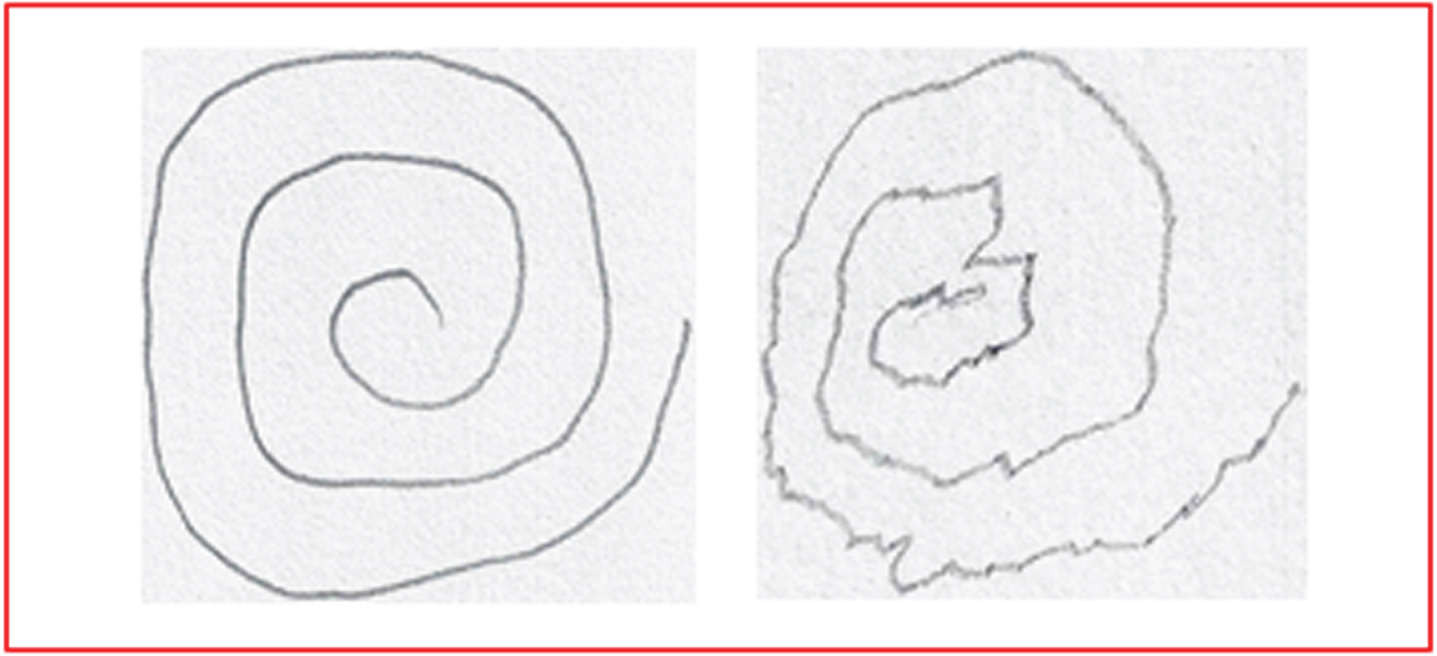
Sample Images of Healthy (Left) and Parkinson (Right).

3.2 Data augmentation layer

Three forms of data augmentation procedures in incorporated in this study. Hybrid Workflow Architecture –I (HWA-I) incorporates online data augmentation. Hybrid Workflow Architecture –II (HWA-II) incorporates offline data augmentation and Hybrid Workflow Architecture –III (HWA-III) incorporates online and offline data augmentation.

3.2.1 Online data augmentation

The online data augmentation is the real-time data augmentation and it is the default option for AI models. The main operation of augmentation is performed in random basis and the augmented data is not stored in the disk or cloud. The workflow of online data augmentation:

Step 1: Load the input images

Step 2: Perform the operation of random augmentation.

Step 3: Train the AI model directly with augmented images.

3.2.2 Offline data augmentation

The offline data augmentation is the generation and storage of augmented images. This type of augmentation is mostly preferred as it gives the opportunity to store and view augmented images which eventually provides a validation about the quality of the augmented image by the human end manually.

Step 1: Load the input images

Step 2: Generate and store augmented image using dataset generator function.

Step 3: Load the augmented images

Step 4: Train the model using the data in Step 3.

3.2.3 Hybrid data augmentation

The integration of offline and online data augmentation is known as hybrid data augmentation.

Step 1: Load the input images

Step 2: Generate and store the augmented images using data generator function

Step 3: Load the augmented images

Step 4: Perform the operation of random online augmentation on data procured in step 3

Step 5: Train the AI model directly with augmented images.

3.3 Data processing and sampling layer

Data Processing and Sampling Layer consists of two prominent processes namely annotation and training-testing split. Annotation is the process of labelling the images based on the class labels. The class labels correspond to 0 and 1 which indicates healthy and Parkinson subjects respectively. Training and Testing split is the process of dividing the data into training and testing samples for training and evaluating the model. The ratio of training and testing sample followed is 80: 20.

3.4 Feature extraction layer

The feature extraction is the vital layer and for robust feature extraction process, DenseNet 201, a Transfer Learning (TL) method is incorporated in the proposed system by only utilizing the feature extraction layers and not utilizing the classification layer. The Keras framework is used to incorporate DenseNet 201for feature extraction and the fully connected layer (include-top) parameter in DenseNet 201 keras package is set to “False” as the novel classification layer is customized separately in the proposed system architecture and the pre-built classification layer in the pretrained model is not used for proposed system architecture. The DenseNet 201 is a Convolutional Neural Network (CNN) based pre-trained model with 201 deep layers and it consists of dense blocks, convolution and pooling layers. The dense blocks are preceded by a convolution layer with 7 x 7 convolution size and a max pooling layer with 3 x 3 kernel size.

3.4.1 Dense blocks

It is used for down sampling which transforms the size of feature maps. The output after applying filter or any computation to an image is known as feature maps.

3.4.2 Transition Layers

The transition layer is present be-tween two dense blocks. The Batch Normalization (BN), convolution and pooling layers are collectively known as transition layers. The convolution is the process of extracting information from image and producing a feature map by applying a filter which is known as kernel. The convolution layers of kernel size 1 x 1 used in the transition layers which is succeeded by each dense block. The pooling operation is used for dimensionality reduction of feature maps procured after convolution operation. The pooling operation reduces the dimensions of the feature maps by applying average pooling technique which provides the prominent features by averaging the pixel value in the region of feature maps. The average pooling layer of kernel size 2 x 2 is used in the transition layer which is succeeded by each dense block.

The objective function of DenseNet 201 is mathematically defined as: $x_{l} = H_{l} ([x_{1}, x_{2}, \dots \dots, x_{l} - 1])$ (1) Where,

x_l is the output of the lth layer.

[x₁,x₂,……,x_l - 1] is the concatenation of feature maps of each layer.

H_l(.) is the composite function which performs the core functions and non-linear transformation namely the Batch Normalization (BN), Rectified Linear Units (ReLU), Pooling and Convolution layers.

3.5 Classification and evaluation layer

The classification layer consists of 124 dense neurons which is activated using the activation function Rectified Linear Unit (ReLu). The activation functions are used to introduce non- linearity. The output layer consists of two neurons with SoftMax function. The mathematical representation of ReLu is: $ReLU = {\begin{matrix} Z & Z > 0 . \\ 0 & Z < = 0 . \end{matrix}$

Where z is the integer and ReLU activation function returns the maximum integer, the simple formula of ReLU is: $f (Z) = \max (0, z)$ (2) The mathematical representation of Softmax function is:

$σ (Z_{i}) = (\frac{e^{Z_{i}}}{\sum_{j} e^{Z_{j}}}) j = 1, . . ., n$ (3) Where,

sigma is the Softmax

z_i is the input vector

e^Z_i is the standard exponential function of input vector

k is the number of classes in the multi-class classifier

e^Z_j is the standard exponential function of output vector

The evaluation layer evaluates the trained model with testing data using the metrics namely Accuracy, Precision, F1 Score and Recall. The metrics are provided based on the four prominent values namely True Positive (TP), True Negative (TN), False Positive (FN) and False Negative (FN). TP corresponds to the values of correctly predicted positive classes. TN corresponds to the values of correctly predicted negative classes. FP corresponds to the value of misclassified positive classes. FN corresponds to the value of misclassified negative classes. $Accuracy = (TP + TN) / (TP + TN + FP + FN)$ (4) $Precision = TP / (TP + FP)$ (5) $F 1 Score = TP / (TP + FN)$ (6)

$\begin{matrix} Recall = \\ (2 * Precision * Recall) / (Precision + Recall) \end{matrix}$ (7)

Fig. 2

Hybrid Workflow Architecture of the Proposed System

3.6 Algorithm

Table 5 presents the notations and its functionality which used in the construction of algorithm.

3.6.1 Algorithm(Hybrid Workflow Architecture -I)

Input< -Spiral Drawing Test (SDT) Images Dataset Output< -Classification Report

Step: 1 Import the necessary packages

Step: 2 Load the training and test set directories from the source path file(Path) to the directory named (Image_Directory) Image_Directory< -Path

Step: 3 List all the files in the directories

Step: 4 Annotate the Image Files with Class_Labels (0,1):

Image_Directory + = Class_Labels

Step: 5 Split the data into training and testing samples using train_test_split function and store it in four variables –Image_Train_X (holds training data –features), Image_Train_Y(holds training data- labels), Image_Test_X(holds testing data –features) and Image_Test_Y (holds testing data- labels)

Image_Train_X, Image_Train_Y, Image_Test_X, Image_Test_Y < -train_test_split (Image_directory,

Class_Labels, test_size= 0.2, random_state = False)

Table 5
Notations and its Functionality

Notations Functionality

Image_Directory A variable which holds the path where the images are stored.

Class_Labels A variable which holds the values of the label corresponding to each instance present in the data. The values of the label are (0,1). 0 specifies the instances corresponding to healthy subject and 1 specifies the instances corresponding to Parkinson Disorder (PD).

train_test_split() An inbuilt function provided by a python programming language-based library named Scikit. This function splits the samples present in the directory as training and testing data samples wherein training samples is used for AI model training and testing samples is used for testing the trained AI model.

test_size Parameter with single real numerical values present inside the train_test_split function which indicates the size of the test samples for splitting. It is set as 0.2 in this study which indicates 20% of the complete is considered as testing sample and remaining is considered as training sample.

random_state Parameter with Boolean value present inside train_test_split which is a control parameter involved in shuffling of data while splitting. In this study random_state is set to FALSE which means shuffling is not done.

ImageDataGenerator() An inbuilt method provided by the python programming language based library named Keras. This method is used for augmenting data with certain parameters namely horizontal_flip, vertical_flip, Rotation_Image, zoom_range, width_shift_range, height_shift_range, shear_range, fill_mode.

horizontal_flip This parameter is used in ImageDataGenerator() function for augmentation of images by flipping the images in horizontal manner which eventually introduces variations in images. It is a Boolean value-based parameter; therefore, it is set to True in this study.

Vertical_flip This parameter is used in ImageDataGenerator () function for augmentation of images by flipping the images in vertical manner which eventually introduces variations in images. It is a Boolean value-based parameter; therefore, it is set to True in this study.

Rotation_Image This parameter is used in ImageDataGenerator () function for augmentation of images by random rotation of images. The value of Rotation_Image is set to 20 which corresponds to the degree to which the image to be rotated.

Zoom_range This parameter is used in ImageDataGenerator () function for augmentation of images by performing random zooming operation. The Zoom_range value is set to 0.

width_shift_range This parameter is used in ImageDataGenerator () function for augmentation of images by performing shifting operation with respect to width. The value of width is set to 0.2

height_shift_range This parameter is used in ImageDataGenerator () function for augmentation of images by performing shifting operation with respect to width. The value of height is set to 0.3

Shear_range This parameter is used in ImageDataGenerator () function for augmentation of images for rectifying the errors based on perception angles in an image. The value of shear_range is set to 0.1.

fill_mode This parameter is used in ImageDataGenerator () function for augmentation of images by filling the empty spaces obtained after incorporating shifting operation.

Data_Generator_online The variable which holds the ImageDataGenerator () function and its results.

DenseNet201() The function is for feature extraction process. DenseNet201() extracts the prominent features from the image. Dense-Net201() is densely connected convolutional networks.

input_shape This parameter of DenseNet201() function is used to specify the input shape of the DenseNet201(). This parameter is specified as tuple with three values which corresponds to channel, width and height. The value of input_shape set in this study is (100,100,3).

include_top This parameter of DenseNet201() function is used to specify the fully connected layer for classification purpose. It is a Boolean value and it is set to False in this study as customized classification layer is used and the classification layer of DenseNet201() is not used.

weights This parameter of DenseNet201() function is used to specify wights for inputs of each layer. The value of weights is set to ImageNet which denotes the weights obtained for Dense-Net201() after training with ImageNet database.

pooling This parameter of DenseNet201() function is used to obtain the prominent features from the output obtained after the convolution process.

Pretrained_FE_Model The variable which holds the DenseNet201() function and stores the results obtained from DenseNet201() function.

Dense () This function is used for classification. It is the customized classification layer with 124 neurons(computation units).

activation This parameter of Dense () is used to introduce non-linearity in the layers of Dense model.

OutputLayer The final output layer which produces the classification output after Softmax activation operation.

Compile() The entire model workflow is compiled and the training is performed with evaluation using this compile () function.

Optimizer The optimizer parameter is used in compile() function for ensuring the difference between the predicted and actual value.

Loss The metric to evaluate the model, this parameter is present in the compile() function.

Metrics The metrics parameter holds the accuracy value and this parameter is part of compile () function.

Classification_model This variable holds the entire AI model workflow with final inputs and output.

Notations	Functionality
Image_Directory	A variable which holds the path where the images are stored.
Class_Labels	A variable which holds the values of the label corresponding to each instance present in the data. The values of the label are (0,1). 0 specifies the instances corresponding to healthy subject and 1 specifies the instances corresponding to Parkinson Disorder (PD).
train_test_split()	An inbuilt function provided by a python programming language-based library named Scikit. This function splits the samples present in the directory as training and testing data samples wherein training samples is used for AI model training and testing samples is used for testing the trained AI model.
test_size	Parameter with single real numerical values present inside the train_test_split function which indicates the size of the test samples for splitting. It is set as 0.2 in this study which indicates 20% of the complete is considered as testing sample and remaining is considered as training sample.
random_state	Parameter with Boolean value present inside train_test_split which is a control parameter involved in shuffling of data while splitting. In this study random_state is set to FALSE which means shuffling is not done.
ImageDataGenerator()	An inbuilt method provided by the python programming language based library named Keras. This method is used for augmenting data with certain parameters namely horizontal_flip, vertical_flip, Rotation_Image, zoom_range, width_shift_range, height_shift_range, shear_range, fill_mode.
horizontal_flip	This parameter is used in ImageDataGenerator() function for augmentation of images by flipping the images in horizontal manner which eventually introduces variations in images. It is a Boolean value-based parameter; therefore, it is set to True in this study.
Vertical_flip	This parameter is used in ImageDataGenerator () function for augmentation of images by flipping the images in vertical manner which eventually introduces variations in images. It is a Boolean value-based parameter; therefore, it is set to True in this study.
Rotation_Image	This parameter is used in ImageDataGenerator () function for augmentation of images by random rotation of images. The value of Rotation_Image is set to 20 which corresponds to the degree to which the image to be rotated.
Zoom_range	This parameter is used in ImageDataGenerator () function for augmentation of images by performing random zooming operation. The Zoom_range value is set to 0.
width_shift_range	This parameter is used in ImageDataGenerator () function for augmentation of images by performing shifting operation with respect to width. The value of width is set to 0.2
height_shift_range	This parameter is used in ImageDataGenerator () function for augmentation of images by performing shifting operation with respect to width. The value of height is set to 0.3
Shear_range	This parameter is used in ImageDataGenerator () function for augmentation of images for rectifying the errors based on perception angles in an image. The value of shear_range is set to 0.1.
fill_mode	This parameter is used in ImageDataGenerator () function for augmentation of images by filling the empty spaces obtained after incorporating shifting operation.
Data_Generator_online	The variable which holds the ImageDataGenerator () function and its results.
DenseNet201()	The function is for feature extraction process. DenseNet201() extracts the prominent features from the image. Dense-Net201() is densely connected convolutional networks.
input_shape	This parameter of DenseNet201() function is used to specify the input shape of the DenseNet201(). This parameter is specified as tuple with three values which corresponds to channel, width and height. The value of input_shape set in this study is (100,100,3).
include_top	This parameter of DenseNet201() function is used to specify the fully connected layer for classification purpose. It is a Boolean value and it is set to False in this study as customized classification layer is used and the classification layer of DenseNet201() is not used.
weights	This parameter of DenseNet201() function is used to specify wights for inputs of each layer. The value of weights is set to ImageNet which denotes the weights obtained for Dense-Net201() after training with ImageNet database.
pooling	This parameter of DenseNet201() function is used to obtain the prominent features from the output obtained after the convolution process.
Pretrained_FE_Model	The variable which holds the DenseNet201() function and stores the results obtained from DenseNet201() function.
Dense ()	This function is used for classification. It is the customized classification layer with 124 neurons(computation units).
activation	This parameter of Dense () is used to introduce non-linearity in the layers of Dense model.
OutputLayer	The final output layer which produces the classification output after Softmax activation operation.
Compile()	The entire model workflow is compiled and the training is performed with evaluation using this compile () function.
Optimizer	The optimizer parameter is used in compile() function for ensuring the difference between the predicted and actual value.
Loss	The metric to evaluate the model, this parameter is present in the compile() function.
Metrics	The metrics parameter holds the accuracy value and this parameter is part of compile () function.
Classification_model	This variable holds the entire AI model workflow with final inputs and output.

Step: 6 Augmenting the data using online augmentation method named as ImageDataGenerator() with appropriate parameters and stores the augmented data (increased data) in the variable named

Data_Generator_Online

Data_Generator_Online < - ImageDataGenerator (horizontal_flip&Tmacr;rue, Vertical_Flip&Tmacr;rue, Rotation_Image = 20, zoom_range = 0, width_shift_range = 0.2, height_shift_range = 0.3, shear_range =0.1, fill_mode = “nearest”)

Step: 7 Extracting the important features from the image using the DenseNet201 pre-trained model method with appropriate parameters and by setting the include_top = False (Performs only extraction and no classification) and store the extracted features in the variable named Pre-trained_FE_Model.

Pretrained_FE_Model< - DenseNet201(input_shape= (100,100,3), include_top=False, weights= ‘ImageNet’, pooling = ‘avg’)

Pretrained_FE_Model< - False

Step: 8 Perform classification using the customized Deep Learning (DL) model.

Step 8.1 Feed the input (features extracted –stored in variable named –Pre-trained_FE_Model.input) to the input layer variable named as “Input”. Input< - Pre-trained_FE_Model.input.

Step 8.2 Add hidden layer with the variable named Layer using Dense neurons (computational unit) along with the activation function Rectified Linear Unit (ReLU) and the output from the input layer (multiplying with weights to the “Input”) which is stored with the variable Pretrained_FE_Model.output

Layer< - Dense (128, activation = ‘relu’) (Pretrained_FE_Model.output)

Step 8.3 Add output layer with the variable named OutputLayer using 2 Dense neurons along with the softmax activation function.

OutputLayer < - Dense (2, activation = ‘softmax’) (Layer)

Step 8.4 Fit the Model and store the trained model in the variable named Classification_Model and evaluate the model by compiling with the evaluation parameters namely adam optimizer, catergorical_crossentropy loss function and accuracy metric

Classification_Model< - Model (inputs = Input, outputs = OutputLayer)

Classification_Model.compile (optimizer = ‘adam’, loss = ‘categorical_crossentropy’, metrics = [‘accuracy’])

3.6.2 Algorithm (Hybrid Workflow Architecture -II)

Input< - Spiral Drawing Test (SDT) Images Dataset

Output< - Classification Report

Step: 1 Import the necessary packages

Step: 2 Load the training and test set directories from the source path file (Path) to the directory named (Image_Directory)

Image_Directory < - Path

Step: 3 List all the files in the directories

Step: 4 Augmenting the images using offline augmentation using the source files in the directories.

Image< - load_img(path)

Input_Image< - img_to_array (Image)

Input_Image< - Input_Image. reshape ((1,) +

Input_Image_array. shape)

Data_Generator < - ImageDataGenerator (rotation_range = 40, shear_range = 0.1, zoom_range = 0.1, horizontal_flip = True, brightness_range = (0.5, 1.5))

Image_Sample_Count = 0

For Image_Batch in Data_Generator.flow(Input_Image, batch_size = 1, save_to_dir = path, save_prefix = name,save_format = ‘jpeg’)

Image_Sample_Count + = 1

If Image_Sample_Count >50:

Then Break

Step: 5 Store the Augmented Images in Disk

Step: 6 Load the training and test set directories from the source path file (Path) to the directory named (Image_Directory)

Image_Directory < - Path

Step: 7 List all the files in the directories

Step: 8 Annotate the Image Files with Class_Labels (0,1):

Image_Directory + = Class_Labels

Step: 9 Split the data into training and testing samples using train_test_split function and store it in four variables –Image_Train_X (holds training data –features),Image_Train_Y (holds training data- labels), Image_Test_X(holds testing data –features) and Image_Test_Y (holds testing data-labels)

Image_Train_X, Image_Train_Y, Image_Test_X, Image_Test_Y < - train_test_split (Image_directory, Class_Labels,test_size= 0.2,random_state = False)

Step: 10 Extracting the important features from the image using the DenseNet201 pre-trained model method with appropriate parameters and by setting the include_top = False (Performs only extraction and no classification) and store the extracted features in the variable named Pretrained_FE_Model.

Pretrained_FE_Model < - DenseNet201(input_shape= (100,100,3), include_top=False, weights= ‘ImageNet’, pooling = ‘avg’)

Pretrained_FE_Model< - False

Step: 11 Perform classification using the customized Deep Learning (DL) model. Step: 11.1 Feed the input (features extracted –stored in variable named –Pretrained_FE_Model.input) to the input layer variable named as “Input”. Input < - Pretrained_FE_Model.input

Step 11.2 Add hidden layer with the variable named Layer using Dense neurons (computational unit) along with the activation function Rectified Linear Unit (ReLU) and the output from the input layer (multiplying with weights to the “Input”) which is stored with the variable Pretrained_FE_Model.output Layer< - Dense (128, activation = ‘relu’) (Pretrained_FE_Model.output)

Step: 11.3 Add output layer with the variable named OutputLayer using 2 Dense neurons along with the softmax activation function. OutputLayer< - Dense (2, activation = ‘softmax’) (Layer)

Step: 11.4 Fit the Model and store the trained model in the variable named Classification_Model and evaluate the model by compiling with the evaluation parameters namely adam optimizer, catergorical_crossentropy loss function and accuracy metric. Classification_Model < - Model (inputs = Input, outputs = OutputLayer)

Classification_Model.compile (optimizer = ‘adam’, loss =‘categorical_crossentropy’, metrics = [‘accuracy’])

3.6.3 Algorithm (Hybrid Workflow Architecture -III)

Input< - Spiral Drawing Test (SDT) Images Dataset

Output< - Classification Report

Step: 1 Import the necessary packages

Step: 2 Load the training and test set directories from the source path file (Path) to the directory named (Image_Directory)

Image_Directory < - Path

Step: 3 List all the files in the directories

Step: 4 Augmenting the images using offline augmentation using the source files in the directories.

Image < - load_img(path)

Input_Image < - img_to_array (Image)

Input_Image < - Input_Image. reshape ((1,) + Input_Image_array.shape)

Data_Generator < - ImageDataGenerator (rotation_range = 40, shear_range = 0.1, zoom_range = 0.1,horizontal_flip = True, brightness_range = (0.5, 1.5))

Image_Sample_Count = 0

For Image_Batch in Data_Generator.flow(Input_Image, batch_size = 1, save_to_dir = path, save_prefix = name,save_format = ‘jpeg’)

Image_Sample_Count + = 1

If Image_Sample_Count >50:

Then Break

Step: 5 Store the Augmented Images in Disk

Step: 6 Load the training and test set directories from the source path file (Path) to the directory named (Image_Directory)

Image_Directory < - Path Step: 7 List all the files in the directories

Step: 8 Annotate the Image Files with Class_Labels (0,1):

Image_Directory + = Class_Labels

Step: 9 Split the data into training and testing samples using train_test_split function and store it in four variables –Image_Train_X (holds training data –features),

Image_Train_Y(holds training data- labels),

Image_Test_X(holds testing data –features) and

Image_Test_Y (holds testing data- labels)

Image_Train_X, Image_Train_Y, Image_Test_X, Image_Test_Y < -train_test_split (Image_directory,

Class_Labels,test_size= 0.2, random_state = False)

Step: 10 Augmenting the data using online augmentation method named as ImageDataGenerator()

with appropriate parameters and stores the augmented data (increased data)

in the variable named Data_Generator_Online

Data_Generator_Online < - ImageDataGenerator (horizontal_flip= True, Vertical_Flip = True, Rotation_Image = 20, zoom_range = 0, width_shift_range = 0.2, height_shift_range = 0.3, shear_range =0.1, fill_mode = “nearest”)

Step: 11 Extracting the important features from the image using the DenseNet201 pre-trained model method with appropriate parameters and by setting the include_top = False (Performs only extraction and no classification) and store the extracted features in the variable named Pretrained_FE_Model.

Pretrained_FE_Model < - DenseNet201(input_shape= (100,100,3), include_top=False, weights= ‘ImageNet’, pooling = ‘avg’)

Pretrained_FE_Model< - False

Step: 12 Perform classification using the customized Deep Learning (DL) model.

Step: 12.1 Feed the input (features extracted –stored in variable named –Pretrained_FE_Model.input) to the input layer variable named as “Input”. Input < - Pretrained_FE_Model.input

Step: 12.2 Add hidden layer with the variable named Layer using Dense neurons (computational unit) along with the activation function Rectified Linear Unit (ReLU) and the output from the input layer (multiplying with weights to the “Input”) which is stored with the variable Pretrained_FE_Model.output Layer < - Dense (128, activation = ‘relu’)

(Pretrained_FE_Model.output)

Step: 12.3 Add output layer with the variable named OutputLayer using 2 Dense neurons along with the softmax activation function.

OutputLayer< - Dense (2, activation = ‘softmax’) (Layer)

Step: 12.4 Fit the Model and store the trained model in the variable named Classification_Model and evaluate the model by compiling with the evaluation parameters namely adam optimizer, catergorical_crossentropy loss function and accuracy metric

Classification_Model < - Model (inputs = Input, outputs = OutputLayer)

Classification_Model.compile (optimizer = ‘adam’, loss= ’categorical_crossentropy’, metrics = [‘accuracy’])

4 Result analysis

4.1 Macro average result analysis

Table 6 presents the Macro Average of Precision, Recall and F1 score values of six experiments for each Hybrid Workflow Architectures.

Inferences from Table 6:

i. Hybrid Workflow Architecture- I(HWA-I): The highest Macro Average Precision value is 0.93 in experiment 2, highest Macro Average Recall Value is 0.94 in experiment 2 and the highest Macro Average F1 Score is 0.93.

ii. Hybrid Workflow Architecture –II (HWA-II): The highest Macro Average Precision value is 0.98 in all experiments; highest Macro Average Recall Value is 0.98 in all experiments and the highest Macro Average F1 Score is 0.98.

iii.Hybrid Workflow Architecture-III (HWA-III): The highest Macro Average Precision Value is 0.97 in experiment 6, highest Macro Average Recall Value is 0.97 in experiment 6 and the highest Macro Average F1 Score is 0.97.

Table 6
Macro Average –Precision, Recall, F 1 score

Architecture EXP_NO Precision Macro-Average Recall Macro Average F1 Score Macro Average

Hybrid Workflow Architecture-I (HWA-I) 1 0.79 0.81 0.80

2 0.93 0.94 0.93

3 0.86 0.86 0.86

4 0.88 0.89 0.87

5 0.88 0.89 0.87

6 0.88 0.89 0.87

Hybrid Workflow Architecture-II (HWA-II) 1 0.98 0.98 0.98

2 0.98 0.98 0.98

3 0.98 0.98 0.98

4 0.98 0.98 0.98

5 0.98 0.89 0.98

6 0.98 0.98 0.98

Hybrid Workflow Architecture-III (HWA-III) 1 0.95 0.95 0.95

2 0.95 0.95 0.95

3 0.94 0.94 0.94

4 0.94 0.94 0.94

5 0.95 0.95 0.94

6 0.97 0.97 0.97

Architecture	EXP_NO	Precision Macro-Average	Recall Macro Average	F1 Score Macro Average
Hybrid Workflow Architecture-I (HWA-I)	1	0.79	0.81	0.80
	2	0.93	0.94	0.93
	3	0.86	0.86	0.86
	4	0.88	0.89	0.87
	5	0.88	0.89	0.87
	6	0.88	0.89	0.87
Hybrid Workflow Architecture-II (HWA-II)	1	0.98	0.98	0.98
	2	0.98	0.98	0.98
	3	0.98	0.98	0.98
	4	0.98	0.98	0.98
	5	0.98	0.89	0.98
	6	0.98	0.98	0.98
Hybrid Workflow Architecture-III (HWA-III)	1	0.95	0.95	0.95
	2	0.95	0.95	0.95
	3	0.94	0.94	0.94
	4	0.94	0.94	0.94
	5	0.95	0.95	0.94
	6	0.97	0.97	0.97

4.2 Weighted average results analysis

Table 7 presents the Weighted Average of Precision, Recall and F1 score values of six experiments for each Work-flow Architectures.

Inferences from Table 7:

Table 7
Weighted Average –Precision, Recall, F 1 score

Architecture EXP_NO Precision Weighted-Average Recall Weighted Average F1 Score Weighted Average

Hybrid Workflow Architecture-I (HWA-I) 1 0.81 0.80 0.80

2 0.87 0.87 0.87

3 0.87 0.87 0.87

4 0.87 0.87 0.87

5 0.87 0.87 0.87

6 0.90 0.89 0.87

Hybrid Workflow Architecture-II (HWA-II) 1 0.98 0.98 0.98

2 0.98 0.98 0.98

3 0.98 0.98 0.98

4 0.98 0.98 0.98

5 0.98 0.89 0.98

6 0.98 0.98 0.98

Hybrid Workflow Architecture-III (HWA-III) 1 0.95 0.95 0.95

2 0.95 0.95 0.95

3 0.94 0.94 0.94

4 0.94 0.94 0.94

5 0.95 0.94 0.94

6 0.97 0.97 0.97

Architecture	EXP_NO	Precision Weighted-Average	Recall Weighted Average	F1 Score Weighted Average
Hybrid Workflow Architecture-I (HWA-I)	1	0.81	0.80	0.80
	2	0.87	0.87	0.87
	3	0.87	0.87	0.87
	4	0.87	0.87	0.87
	5	0.87	0.87	0.87
	6	0.90	0.89	0.87
Hybrid Workflow Architecture-II (HWA-II)	1	0.98	0.98	0.98
	2	0.98	0.98	0.98
	3	0.98	0.98	0.98
	4	0.98	0.98	0.98
	5	0.98	0.89	0.98
	6	0.98	0.98	0.98
Hybrid Workflow Architecture-III (HWA-III)	1	0.95	0.95	0.95
	2	0.95	0.95	0.95
	3	0.94	0.94	0.94
	4	0.94	0.94	0.94
	5	0.95	0.94	0.94
	6	0.97	0.97	0.97

i. Hybrid Workflow Architecture- I(HWA-I): The highest Weighted Average Precision value is 0.94 in experiment 2, highest Weighted Average Recall Value is 0.93 in experiment 2 and the highest Weighted Average F1 Score is 0.93.

ii. Hybrid Workflow Architecture –II (HWA-II): The highest Weighted Average Precision value is 0.98 in all experiments; highest Weighted Average Recall Value is 0.98 in all experiments and the highest Weighted Average F1 Score is 0.98.

iii. Hybrid Workflow Architecture-III (HWA-III): The highest Weighted Average Precision Value is 0.97 in experiment 6, high-est Weighted Average Recall Value is 0.97 in experiment 6 and the highest Weighted Average F1 Score is 0.97.

4.3 Accuracy and loss value results analysis

Table 8 presents the accuracy values of six experiments for each Workflow Architectures (WA).

Inferences from Table 8:

i. Hybrid Workflow Architecture- I (HWA-I): The highest accuracy 0.93 is obtained in experiment 2 with hyperparameters epochs=50 and batch size=64.

ii. Hybrid Workflow Architecture-II (HWA-II): The highest accuracy 0.98 is obtained in all six experiments with all possible hyperparameters value.

iii.Hybrid Workflow Architecture-III(HWA-III): The highest accuracy 0.97 is obtained in experiment 6.

Table 8
Accuracy of Eighteen Experiments

Architecture EXP.NO Conditions Accuracy

Epochs Batch Size

Hybrid Workflow Architecture-I (HWA-I) 1 50 32 0.80

2 50 64 0.93

3 50 128 0.87

4 100 32 0.87

5 100 64 0.87

6 100 128 0.87

Hybrid Workflow Architecture-II (HWA-II) 7 50 32 0.98

8 50 64 0.98

9 50 128 0.98

10 100 32 0.98

11 100 64 0.98

12 100 128 0.98

Hybrid Workflow Architecture-III (HWA-III) 13 50 32 0.95

14 50 64 0.95

15 50 128 0.94

16 100 32 0.94

17 100 64 0.94

18 100 128 0.97

Architecture	EXP.NO	Conditions	Accuracy
Hybrid Workflow Architecture-I (HWA-I)	1	50	32	0.80
	2	50	64	0.93
	3	50	128	0.87
	4	100	32	0.87
	5	100	64	0.87
	6	100	128	0.87
Hybrid Workflow Architecture-II (HWA-II)	7	50	32	0.98
	8	50	64	0.98
	9	50	128	0.98
	10	100	32	0.98
	11	100	64	0.98
	12	100	128	0.98
Hybrid Workflow Architecture-III (HWA-III)	13	50	32	0.95
	14	50	64	0.95
	15	50	128	0.94
	16	100	32	0.94
	17	100	64	0.94
	18	100	128	0.97

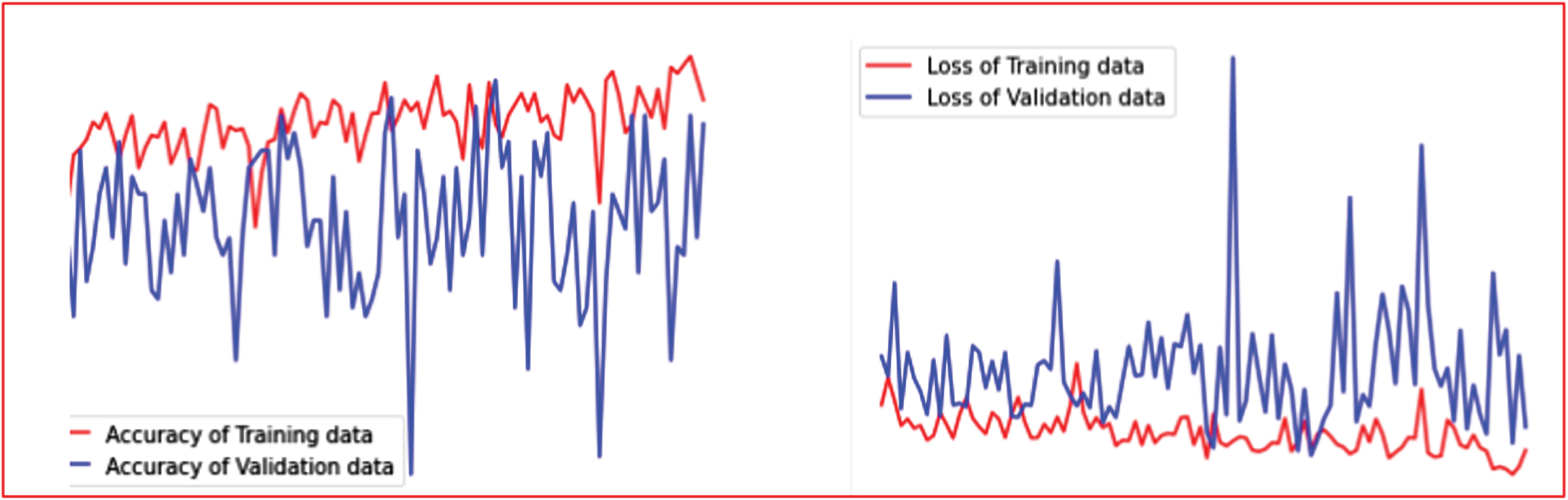
Figure 3 presents the accuracy and loss graph of the best result for Hybrid Workflow Architecture (HWA-I). The accuracy graph depicts that the training accuracy is higher than the testing accuracy. The main reason for possible overfitting in this HWA-I is the data augmentation layer which incorporates online data augmentation method with less data images.

Fig. 3

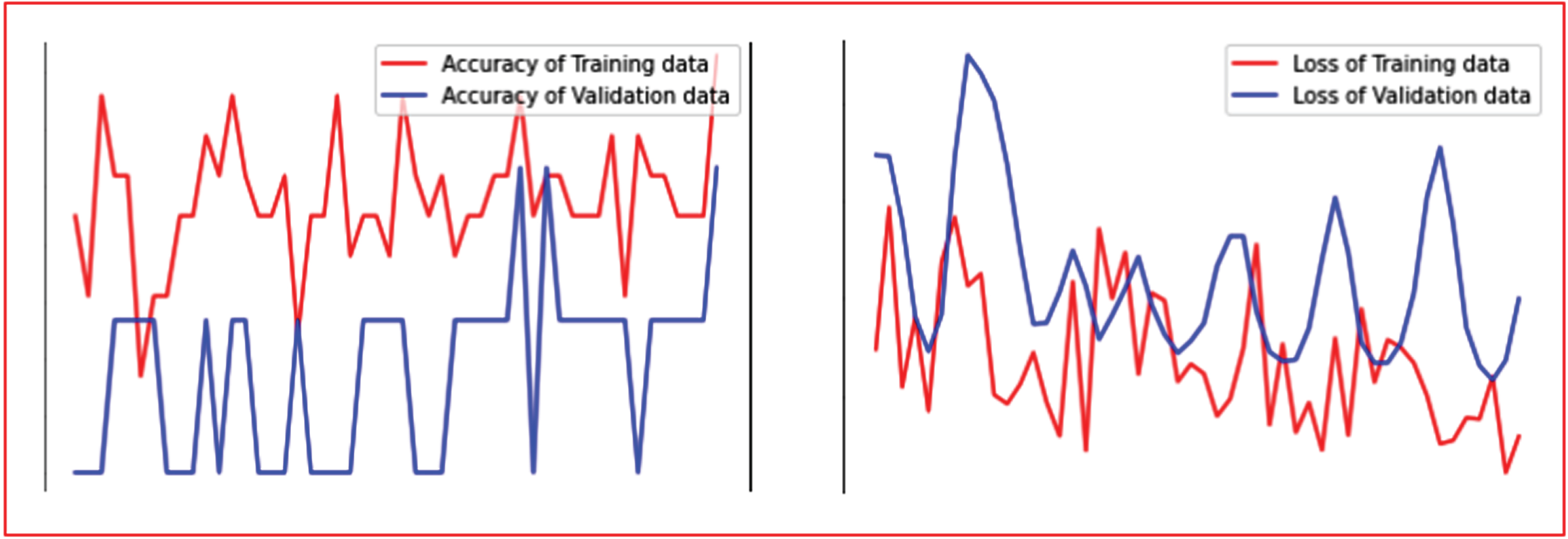
Accuracy and Loss Graph (Best Results) of Hybrid Workflow Architecture-I.

Figure 4 presents the accuracy and loss graph of the best result for Hybrid Workflow Architecture (HWA-II). The accuracy graph depicts that the training accuracy is higher than the testing accuracy. The main reason for possible overfitting is the data being slight bias due to offline data augmentation procedure.

Fig. 4

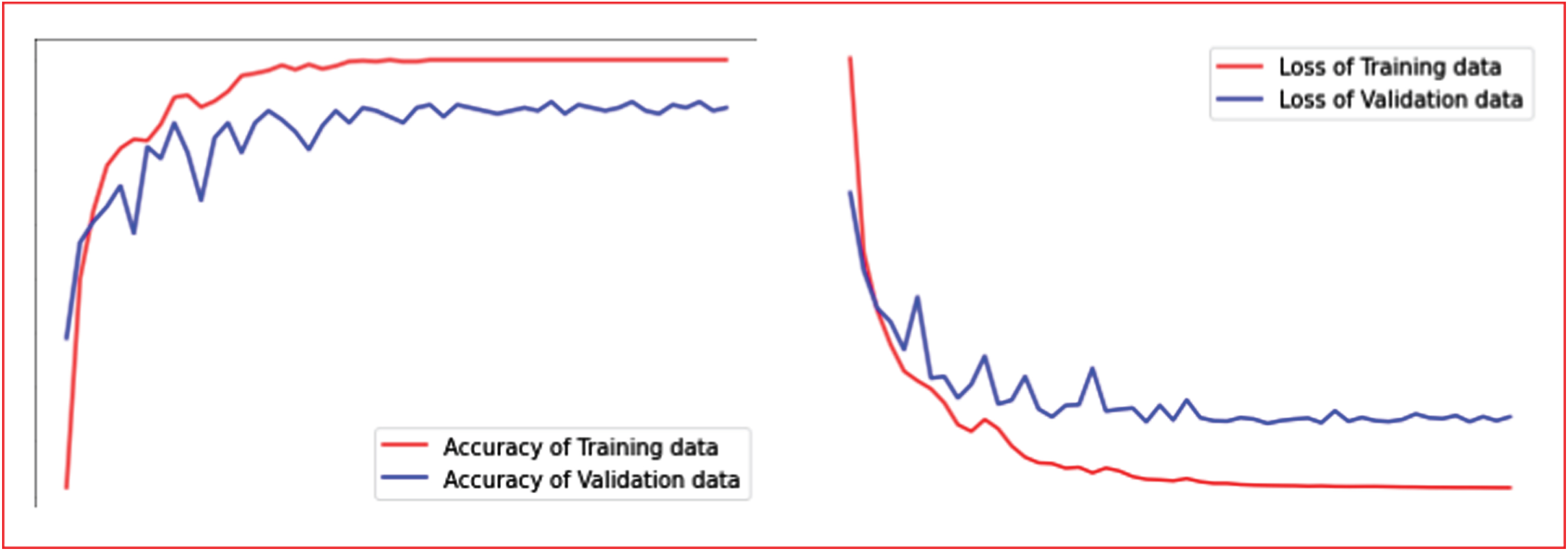
Accuracy and Loss Graph (Best Results) of Hybrid Workflow Architecture-II.

Figure 5 presents the accuracy and loss graph of the best result of Hybrid Workflow Architecture-III (HWA-III). The accuracy of training and testing graph is balanced in all epochs which clearly indicates that the model is well trained with the novel hybrid data augmentation procedure-based data and the accuracy is reliable.

Fig. 5

Accuracy and Loss Graph (Best Results) of Hybrid Workflow Architecture-III.

4.4 Main findings and inferences

a) Accuracy Metric Analysis: This metric provides the overall performance of model since it provides the value based on the total number of classes present in the dataset which corresponds to healthy and PD. The highest accuracy of 98% is provided by HWA-II. Therefore, the workflow followed in this architecture is more reliable in discriminating the healthy subject and PD. The most important core layer of the HWA-II architecture is the offline data augmentation layer which augments data and stores data offline which increased the data size and also the quality of the AI model performance with respect to discriminating healthy and PD with high number of corrected prediction due to offline data loading.

b) Precision, Recall and F1 score Marco and Weighted Analysis:The highest value is obtained by HWA-II and the second highest value is obtained by HWA-III. The highest precision value indicates the model capacity to predict positive instances (PD subjects). The HWA-II is able to perform accurate positive prediction (PD subjects’ prediction) as per the precision value obtained in Macro and weighted analysis. The recall metric corresponds to the model’s ability to detect positive samples and it is perfectly done by HWA-II and HWA-III. The misdiagnosis rate is less in HWA-II compared to HWA-I and HWA-III and the misdiagnosis rate is less in HWA-II compared to HWA-III.

c) The empirical results of this study reveal a key finding that offline augmentation process in HWA-II or offline augmentation process integrated with online augmentation process in HWA-III provides a reliable rate of discrimination between healthy and PD subjects and reduces the misdiagnosis rate.

d) The main reason of reliable results is that the proposed study has provided three different Hybrid Workflow Architectures for PD diagnosis based on SDT with reliable accuracy combination of core layers are designed in such a way that: i. The data is of good quantity by introducing the data augmentation layers with three different combinations.

ii. Inputs to the classification model with good variance and less redundant which has been made possible by incorporating TL based feature extraction process.

iii. The outputs to be prediction with reliability which is made possible by incorporating customized classification layer with carefully choosing of activation functions.

e) From the results it is well recommended that SDT can be used as a modality for PD prediction with the proposed Hybrid Workflow Architectures (HWA).

4.5 Pros analysis

a) The construction of workflow architectures in hybrid manner provides high reliability and robustness as the proposed system attempted in developing three hybrid workflow architecture which makes this study progressive and stands out in novelty when compared to existing system.

b) The hyperparameter experimental setup for empirical study to analyze results provides an effective validation method as hyperparameter is the prominent parameter value for the AI model for convergence to decision making (i.e., final PD prediction).

4.6 Limitation analysis

a) The proposed system provides good results in PD prediction based on SDT image modality, but single modality cannot provide enough validation when compared to the multiple modality-based PD prediction. The lack of multiple modality incorporation for PD prediction is one of the limitations.

b) The classification between PD and healthy subject is focused in the proposed study and the study is restricted to tremor symptom of PD and there is a high need to develop model which distinguishes between the tremor symptom of PD and other tremor symptom in order to have a specialized system for PD diagnosis.

5 Conclusion

A diagnosis system for Parkinson’s Disorder (PD) requires the identification of clinical markers at a low or no misdiagnosis rate. The proposed system reduced the research gaps found in the literature survey by implementing three hybrid workflow architectures. The key contribution and novelty of the proposed system are the implementation of three hybrid workflow architectures integrated with hyperparameter experimentation. The proposed system provided the highest accuracy (98%), Macro Precision (0.98), Macro F1 score (0.98), Macro Recall (0.98), Weighted Precision (0.98), Macro F1 score (0.98), and Weighted Re-call (0.98). Analysis of the results shows that the proposed system is reliable for PD diagnosis. It can be concluded that the Spiral Drawing Test (SDT) is an efficient clinical marker for the early diagnosis of PD integrated with an AI system. The limitation of the proposed work is the lack of integration of multiple modalities for creation of robust model. Future work will leverage various Transfer Learning (TL) methods for the feature extraction process with acquisition of multi-modality data.

References

Pringsheim

, Jette

, Frolkis

and Steeves

T.D.

, Theprevalence of Parkinson’s disease: a systematic review andmeta-analysis, Mov Disord 29(13) (2014), 1583–90 10.1002/mds.25945. Epub 2014 Jun 28. PMID: 24976103

Chakraborty

, Aich Jong-Seong-Sim

, Han

, Park

, Kim

H.-C.

Parkinson’s Disease Detection from Spiral and Wave Drawings using Convolutional Neural Networks: A Multistage Classifier Approach, 22nd International Conference on Advanced Communication Technology (ICACT), Phoenix Park, Korea (South), 2020, pp. 298–303, doi: 10.23919/ICACT48636.2020.9061497.

San Luciano

, Wang

, Ortega

R.A.

, Yu

, Boschung

and Soto-Valencia

, Digitized Spiral Drawing: A Possible Biomarker forEarly Parkinson’s Disease,, PLoS ONE 11(10), e0162799.

Megha Kamble , Prashant Shrivastava , Megha Jain , Digitized spiraldrawing classification for Parkinson’s disease diagnosis, Measurement: Sensors 16 (2021), 100047. ISSN 2665-9174, https://doi.org/10.1016/j.measen.2021.1000478

Sarah Fan

et al. Early Detection of Parkinson’s Disease Using Machine Learning and Convolutional Neural Networks from Drawing Movements, Computer Science & Information Tech-nology (CS & IT) pp. 291-301.

Gil-Martín

, Montero

J.M.

and San-Segundo

, Parkinson’sDisease Detection from Drawing Movements Using Convolutional, Electronics 8 (2019), 907. https://doi.org/10.3390/electronics8080907

Zhu Li , Jiayu Yang , Yanwen Wang , Miao Cai , Xiaoli Liu , Kang Lu , Early diagnosis of Parkinson’s disease using Continuous ConvolutionNetwork: Handwriting recognition based on off-line hand drawingwithout template, Journal of Biomedical Informatics 130(2022) (1040), 104085. ISSN15320464 https://doi.org/10.1016/j.jbi.2022.104085

Elli Valla , Sven Nõmm , Kadri Medijainen , Pille Taba , AaroToomela Tremor-related feature engineering for machine learningbased Parkinson’s disease diagnostics, Biomedical SignalPro-cessing and Control 75 (2022), 103551, ISSN 1746-8094 https://doi.org/10.1016/j.bspc.2022.103551

Iqra Kamran , Saeeda Naz , Imran Razzak , Muhammad Imran , Handwriting dynamics assessment using deep neural network for earlyidentification of Parkinson’s disease, Future GenerationComputer Systems 117 (2021), 234–244. ISSN 0167-739X.

10.

Kotsavasiloglou

, Kostikis

, Hristu-Varsakelis

and Arnaoutoglou

, Machine learning-based classification of simpledrawing movements in Parkinson’s disease, Biomedical SignalProcessing and Control 31 (2017), 174–180. ISSN 1746 8094.

11.

Moises Diaz , Miguel Angel Ferrer , Donato Impedovo , Giuseppe Pirlo , Gennaro Ves-sio , Dynamically enhanced static handwritingrepresentation for Parkinson’s disease detection, PatternRecognition Letters 128 (2019), 204–210. ISSN 0167-8655.

12.

Shoujiang Xu , Zhigeng Pan , A novel ensemble of random forest forassisting diagnosis of Parkinson’s disease on small handwrittendynamics dataset, International Journal of Medical Informatics 144 (2020), 104283. ISSN1386-5056.

13.

Peter Drotár , Jiří Mekyska , Irena Rektorová , LuciaMasarová , Zdeněk Smékal , Marcos Faundez-Zanuy, , Evaluation of handwriting kinematics and pressure for differentialdiagnosis of Parkinson’s disease, Artificial Intelligence inMedicine 67 (2016), 39–46, ISSN 0933-3657. https://doi.org/10.1016/j.artmed.2016.01.004.

14.

Ayse Betul Oktay , Abdulkadir Kocer Differential diagnosis ofParkinson and essential tremor with convolutional LSTM networks, Biomedical Signal Processing and Control 56 (2020), 101683, ISSN 1746-8094.

15.

s-Bonilla

, Nöth

, Lopera

and Orozco-ArroyaveAnalysis

J.R.

, evaluation of handwriting in patients with Parkinson’sdisease using kinematic, geometrical, and non-linear features, Computer Methods and Programs in Bio-medicine 173 (2019), 43–52, ISSN 0169-2607.

16.

Gao Huang , Zhuang Liu , Kilian Weinberger

Densely Connected Convolutional Networks, CoRR, 2016, http://arxiv.org/abs/1608.06993

17.

Kaiming He , Xiangyu Zhang , Shaoqing Ren , Jian Sun Deep Residual Learning for Image Recognition, CoRR, 2015.

18.

Olaf Ronneberger , Philipp , Thom-as Brox U-Net: Convolutional Networks for Bio-medical Image Segmentation, CoRR, 2015, arXiv.

19.

Andrew Howard , et al. Searching for MobileNetV3, CoRR, 2019.

20.

Mingxing Tan , Quoc Le

EfficientNet: Rethinking Model Scaling for Convolutional Neural Networks, http://arxiv.org/abs/1905.11946, 2019.

21.

Zham

, Kumar

D.K.

, Dabnichki

, Poosa-padi Arjunan

and Raghav

, Distinguishing Different Stages of Parkin-son’s DiseaseUsing Composite Index of Speed and Pen-Pressure of Sketching aSpiral, Front. Neurol. 8, 435. doi: 10.3389/fneur.2017.00435.

Early diagnosis of Parkinson disorder based on spiral drawing image modalities using hybrid transfer learning architecture

Abstract

Keywords

1 Introduction

1.1 Identification of problems

1.2 Possible solutions

1.3 Motivation

1.5 Contributions of the paper

2 Related works

2.1 Survey based on PD diagnosis using hand-written and sketch drawings image modality

2.2 Survey based on different deep learning and transfer learning methods

2.3 Research gaps

3.1 Data collection layer

Table 4 Number of Samples Directory Sub directory Number of Images Samples Total Samples Training Healthy 36 72 Parkinson 36 Testing Healthy 15 30 Parkinson 15

3.2.1 Online data augmentation

3.2.2 Offline data augmentation

3.2.3 Hybrid data augmentation

3.3 Data processing and sampling layer

3.4 Feature extraction layer

3.4.1 Dense blocks

3.4.2 Transition Layers

3.6.1 Algorithm(Hybrid Workflow Architecture -I)

3.6.3 Algorithm (Hybrid Workflow Architecture -III)

4 Result analysis

4.1 Macro average result analysis

4.5 Pros analysis

4.6 Limitation analysis

5 Conclusion

References

Table 4
Number of Samples

Directory Sub directory Number of Images Samples Total Samples

Training Healthy 36 72

Parkinson 36

Testing Healthy 15 30

Parkinson 15