The numerical solution of fuzzy singular Lyapunov matrix equations

Abstract

Fuzzy singular Lyapunov matrix equations have many applications, but feasible numerical methods to solve them are absent. In this paper, we propose an efficient numerical method for fuzzy singular Lyapunov matrix equations, where A is crisp and semi-stable. In our method, we transform fuzzy singular Lyapunov matrix equation into two crisp Lyapunov matrix equations. Then we solve the least squares solutions of the two crisp Lyapunov matrix equations, respectively. The existence of fuzzy solution is also considered. At last, two small examples are presented to illustrate the validate of the method and two large scale examples that the existing method fails to slove are presented to show the efficiency of the method.

1 Introduction

The singular Lyapunov matrix equation is of the form $\mathit{AX}+{\mathit{XA}}^T=C,$(1) where A = (a _ij ) ∈ R^n×n is semi-stable or Lyapunov stable. A matrix is called stable if the real parts of its eigenvalues are negative; It is called semi-stable if the real parts of most of its eigenvalues are negative with few semi-simple exceptions at zero; It is called Lyapunov stable if real parts of its eigenvalues are non-positive. The Lyapunov matrix equation is widely used in cybernetics, signal processing, dynamical systems and the hydrodynamic stability ([2, 26]). Semi-stable matrix has great effects on the analysis of autonomous systems, matrix second-order systems and switched systems ([4, 22]). With kronecker product, (1) is equivalent to (I ⊗ A + A ⊗ I) Vec (X) = Vec (C) , where Vec (X) is a vector obtained by stacking columns of X. So (1) is singular, if A is semi-stable or Lyapunov stable. Just like the connection between Lyapunov matrix equation with optimal stable control, semistable Lyapunov matrix equation arise from optimal semistable control theory for linear and nonlinear dynamical system ([19, 23]). Semistable Lyapunov matrix equations also appear in chemical reaction system, compartmental systems ([17]), isospectral matrix dynamical systems, and dynamical network systems. They cover a broad spectrum of applications including cooperative control of unmanned air vehicles, autonomous underwater vehicles, distributed sensor networks, air and ground transportation systems, swarms of air and space vehicle formations, and congestion control in communication networks ([16, 18]).

In practical applications, the information we received may fuzzy. So we may obtain fuzzy matrix equations when we use fuzzy numbers as a tool for modeling. With a fuzzy matrix $\tilde{C}$ replacing C in (1), we have a fuzzy singular Lyapunov matrix equation(FSLME): $A\tilde{X}+\tilde{X}{A}^T=\tilde{C},$(2) where $\tilde{X}$ is an unknown fuzzy matrix. Solution of a fuzzy linear system is very different from the crisp one. If the solution method is based on the interval arithmetic, we obtain the classic solution. If the solution method is based on the extension principle, we obtain the extension solution ([5]). The classic solution may not exist, but extension solution always exists ([1]). In [13], an extended method for fuzzy linear equations is proposed, a 2n × 2n crisp linear equations is needed to solve in this method. In [29], Fourier transformation is applied to this method, so solving two n × n crisp linear equations instead of one 2n × 2n crisp linear equations is enough. This method makes solving large scale fuzzy linear system much eaiser. In [12], a different approach to solve fuzzy linear equations is proposed. In this method, three n × n crisp linear equations are needed to solve. In [24], an improvement is done to the method. This improvement need to solve the same two n × n crisp linear equations as ones in [29].

Some numerical methods of solving fuzzy matrix equation come from the methods of solving fuzzy linear equations. These methods ([15, 27]) are constructed by using Kronecker product to convert fuzzy linear matrix equations to fuzzy linear equations. And the fuzzy linear equations is solved by the methods in [12, 29-32]. We call this method as kronecker method in this paper. Kronecker method can solve nonsingular and singular fuzzy matrix equations, but it is infeasible to solve large scale equations because it enlarge the scale of equations very much. There are also some methods ([33, 34]) can deal with singular fuzzy matrix equation AX = B without enlarging the dimension of equations, where A is a crisp matrix, X and B are fuzzy matrices. But these methods can not be applied to solve singular fuzzy Lyapunov matrix eqution. Thus, the existing method to solve fuzzy singular matrix equations is the kronecker method. The other methods of solving fuzzy matrix equation come from the combination of numerical methods of crisp matrix equation and fuzzy arithmetic ([20]). This kind of methods can keep scale of equations unchanged, so they are more efficicent. But since there are very few literature about singular crisp Lyapunov matrix equations, as we known, there are not any efficient methods for singular fuzzy Lyapunov matrix equations. In [11], authors proposed a numerical method to solve large scale unstable crisp Lyapunov matrix equation. So the motivation of this paper is to propose an efficient numerical method for singular fuzzy Lyapunov matrix equation by combining the method in [11] with the idea in [20]. Moreover, conditions of fuzzy solution existence are also studied. As we will see in the part of numerical test, this method is efficient when solving large scale equations.

We assume throughout that the coefficient matrix is a crisp semi-stable or Lyapunov stable. Our technique path is as follows. Firstly, the fuzzy singular Lyapunov matrix equation is transformed into two crisp singular Lyapunov matrix equations without enlarging their scales by using the idea in [20]. Then we employ the approach in [11] to numerically solve the least squares solutions of two crisp singular Lyapunov matrix equations. Finally, the fuzzy solution of the original equation is composed. Moreover, both singular consistent and inconsistent cases are discussed. In the case of the consistent singular system, we only need to solve the least squares solutions of two crisp equations, respectively. In the case of inconsistent singular system, we need to do a projection to get rid of the inconsistent part first, and then to solve the projected equation.

The rest part of this paper is organized as follows. In Section 2, some useful preliminaries are presented. In Section 3, the extension method is derived. In Section 4, the implement details of the extension method are presented. In Section 5, several examples, including large scale examples, are presented.

2 Preliminaries

In this section, some preliminaries are presented. The further detail of these preliminaries can be found in [8, 27].

Definition 2.1. A fuzzy number can be defined by its membership function u : R ↦ [0, 1] which satisfies following requirements:

u is an upper semi-continuous function on R,

u (r) =0 outside some interval [a, d],

for a, b, c, d ∈ R with a ≤ b ≤ c ≤ d satisfies

u (r) is a monotonic increasing function on [a, b],

u (r) is a monotonic decreasing function on [c, d],

u (r) =1, ∀ x ∈ [b, c].

According to Definition 2.1, we can represent a fuzzy number in the following form:

$\tilde{u}\left(r\right)=\{\begin{array}{cc}{u}_L\left(r\right),\hfill & r\in [a,b];\hfill \\ 1,\hfill & r\in [b,c];\hfill \\ u_R\left(r\right),\hfill & r\in [c,d];\hfill \\ 0,\hfill & \text{elsewhere}.\hfill \end{array}$(3) where u _L  : [a, b] ↦ [0, 1] and u _R  : [c, d] ↦ [0, 1] are the left and right membership function of the fuzzy number u, respectively. All fuzzy numbers can be expressed by the formula (3), and an another way to define fuzzy numbers is introduced below.

Definition 2.2. A fuzzy number can be presented by a pair of functions $\left(\underset{\_}{u}\right(r),\overline{u}(r\left)\right)$ , r ∈ [0, 1] which satisfy the following requirements:

$\underset{\_}{u}\left(r\right)$ is a bounded continuous non-decreasing function over [0, 1],

$\overline{u}\left(r\right)$ is a bounded continuous non-increasing function over [0, 1],

$\underset{\_}{u}\left(r\right)\le \overline{u}\left(r\right),\forall r\in [0,1]$ .

Moreover, we call $\underset{\_}{u}\left(r\right)$ (or $\overline{u}\left(r\right)$ ) the pair-left (or pair-right) function. When $\underset{\_}{u}\left(r\right)=\overline{u}\left(r\right),\forall r\in [0,1]$ , the fuzzy number is a crisp number. For example, 2 can be writted as (2, 2). According to Definition 2.2, a trapezoidal fuzzy number can be presented with u (x₀, y₀, α, β) in the form which is similar to (3):

$u\left(r\right)=\{\begin{array}{cc}\frac{1}{\alpha }(x-x_0+\alpha ),\hfill & r\in [x_0-\alpha ,x_0];\hfill \\ 1,\hfill & r\in [x_0,y_0];\hfill \\ \frac{1}{\beta }(y_0-x+\beta ),\hfill & r\in [y_0,y_0+\beta ];\hfill \\ 0,\hfill & \text{elsewhere}.\hfill \end{array}$(4) This form corresponds to $\underset{\_}{u}\left(r\right)=x_0-\alpha +\alpha r$ and $\overline{u}\left(r\right)=y_0+\beta -\beta r$ . When x₀ = y₀, it is a triangular fuzzy number.

The arithmetic operations of fuzzy numbers $\tilde{u}\left(r\right)=\left(\underset{\_}{u}\right(r),\overline{u}(r\left)\right)$ , $\tilde{v}\left(r\right)=\left(\underset{\_}{v}\right(r),\overline{v}(r\left)\right)$ and a real number k are the following:

$\tilde{u}\left(r\right)=\tilde{v}\left(r\right)$ if and only if $\underset{\_}{u}\left(r\right)=\underset{\_}{v}\left(r\right)$ and $\overline{u}\left(r\right)=\overline{v}\left(r\right),\forall r\in [0,1]$ ;

$\tilde{u}\left(r\right)+\tilde{v}\left(r\right)=\left(\underset{\_}{u}\right(r)+\underset{\_}{v}(r),\overline{u}(r)+\overline{v}(r\left)\right),0\le r\le 1$ ;

$k\tilde{u}\left(r\right)=\{\begin{array}{cc}\left(k\underset{\_}{u}\right(r),k\overline{u}(r\left)\right),\hfill & \mathrm{if}k\ge 0\hfill \\ \left(k\overline{u}\right(r),k\underset{\_}{u}(r\left)\right),\hfill & \mathrm{if}k<0\hfill \end{array},0\le r\le 1$ .

(2) can be transformed into the following fuzzy linear equation by using Kronecker product ([25]): $L(·)\mathcal{X}=\mathcal{C}.$ where $L(·)=I\otimes A+A\otimes I,\mathcal{X}=\mathit{Vec}\left(X\right),\mathcal{C}=\mathit{Vec}\left(C\right)$ . When A is stable, the Lyapunov operator L (·) is nonsingular, the unique solution of a large scale stable Lyapunov matrix equation can be obtained on the basis of EXTALG algorithm in [20].

3 The extension method

Let $A^{+}=(a_{\mathit{ij}}^{+}{)}_{n\times n}$ and $A^{-}=(a_{\mathit{ij}}^{-}{)}_{n\times n}$ satisfy:

$\{\begin{array}{c}{a}_{\mathit{ij}}>0⟶a_{\mathit{ij}}^{+}=a_{\mathit{ij}},a_{\mathit{ij}}^{-}=0,\hfill \\ a_{\mathit{ij}}<0⟶a_{\mathit{ij}}^{+}=0,a_{\mathit{ij}}^{-}=-a_{\mathit{ij}}.\hfill \end{array}$

So (A ^T ) ⁺ = (A⁺)  ^T , (A ^T ) ^- = (A^-)  ^T . Let $\tilde{X}=(\underset{\_}{X},\overline{X}),$ where $\underset{\_}{X}=({\underset{\_}{x}}_{\mathit{ij}}{)}_{n\times n}$ and $\overline{X}=({\overline{x}}_{\mathit{ij}}{)}_{n\times n}.$ According to [20], (2) can be transformed into a crisp Lyapunov matrix equation with the scale of (2n × 2n) as follow: $\mathit{SY}+{\mathit{YS}}^T=G,$(5) where $S=\left(\begin{array}{cc}\hfill A^{+}\hfill & \hfill -A^{-}\hfill \\ \hfill -A^{-}\hfill & \hfill A^{+}\hfill \end{array}\right),Y=\left(\begin{array}{cc}\hfill \underset{\_}{X}\hfill & \hfill \overline{X}\hfill \\ \hfill \overline{X}\hfill & \hfill \underset{\_}{X}\hfill \end{array}\right)$ , and $G=\left(\begin{array}{cc}\hfill \underset{\_}{C}\hfill & \hfill \overline{C}\hfill \\ \hfill \overline{C}\hfill & \hfill \underset{\_}{C}\hfill \end{array}\right).$

With several elementary transformations, we have

$\begin{array}{ccc}\hfill S& \hfill =\hfill & \left(\begin{array}{cc}\hfill A^{+}\hfill & \hfill -A^{-}\hfill \\ \hfill -A^{-}\hfill & \hfill A^{+}\hfill \end{array}\right)\hfill \\ \hfill & \hfill ⟶\hfill & \left(\begin{array}{cc}\hfill A^{+}\hfill & \hfill -A^{-}\hfill \\ \hfill A^{+}-A^{-}\hfill & \hfill A^{+}-A^{-}\hfill \end{array}\right)\hfill \\ \hfill & \hfill =\hfill & \left(\begin{array}{cc}\hfill A^{+}\hfill & \hfill -A^{-}\hfill \\ \hfill A\hfill & \hfill A\hfill \end{array}\right)\hfill \\ \hfill & \hfill ⟶\hfill & \left(\begin{array}{cc}\hfill A^{+}+A^{-}\hfill & \hfill -A^{-}\hfill \\ \hfill 0\hfill & \hfill A\hfill \end{array}\right)\hfill \\ \hfill & \hfill =\hfill & \left(\begin{array}{cc}\hfill \left|A\right|\hfill & \hfill -A^{-}\hfill \\ \hfill 0\hfill & \hfill A\hfill \end{array}\right).\hfill \end{array}$

Let (λ, x) be an eigenpair of A. With the fact of |λ||X| = |AX| ≤ |A||X|, S is semi-stable or Lyapunov stable if A is semi-stable or Lyapunov stable, respectively. Thus, (5) is not a stable Lyapunov matrix equation.

Then we discuss the existence of the fuzzy solution of (2). By (5), we can easily find that $A^{+}\underset{\_}{X}-A^{-}\overline{X}+\underset{\_}{X}(A^{+}{)}^T-\overline{X}(A^{-}{)}^T=\underset{\_}{C},$(6) $-A^{-}\underset{\_}{X}+A^{+}\overline{X}+\overline{X}(A^{+}{)}^T-\underset{\_}{X}(A^{-}{)}^T=\overline{C}.$(7)

Let (7) minus (6), we have

$\begin{array}{ccc}\hfill \overline{C}-\underset{\_}{C}& \hfill =\hfill & A^{+}(\overline{X}-\underset{\_}{X})+A^{-}(\overline{X}-\underset{\_}{X})\hfill \\ \hfill & \hfill \hfill & +(\overline{X}-\underset{\_}{X})(A^{+}{)}^T+(\overline{X}-\underset{\_}{X}\left)\right(A^{-}{)}^T\hfill \\ \hfill & \hfill =\hfill & (A^{+}+A^{-})(\overline{X}-\underset{\_}{X})\hfill \\ \hfill & \hfill \hfill & +(\overline{X}-\underset{\_}{X})\left(\right(A^{+}{)}^T+\left(A^{-}{)}^T\right).\hfill \end{array}$(8)

Let $\Delta C=\overline{C}-\underset{\_}{C},\Delta X=\overline{X}-\underset{\_}{X}$ , so (8) can be written as the following Lyaunov matrix equation: $\left|A\right|\Delta X+\Delta X|A{|}^T=\Delta C.$(9)

Applying the Kronecker product to (9), we can obtain that $(I_n\otimes |A|+|A|\otimes I_n)\mathit{Vec}\left(\Delta X\right)=\mathit{Vec}\left(\Delta C\right).$(10)

It is clear that the solution of (10) is unique if (I _n  ⊗ |A| + |A| ⊗ I _n ) is nonsingular. However, we should note that |A| may singular.

Proposition 3.1. For an arbitrary fuzzy matrix $\tilde{C}$ , the solution or the least squares solution of (2) is a fuzzy matrix if and only if A is a diagonal matrix.

Proof. Supposed that the matrix A is a semi-stable matrix with rank r, we know that the necessary and sufficient condition for the existence of the solution or the least squares solution of the matrix equations (2) is (I ⊗ |A| + |A| ⊗ I) ⁺ ≥ 0. Then we need to show that (I ⊗ |A| + |A| ⊗ I) ⁺ ≥ 0 if and only if A is a diagonal matrix.

Firstly supposed (I ⊗ |A| + |A| ⊗ I) ⁺ ≥ 0 holds, so that we can obtain the equation (I ⊗ |A| + |A| ⊗ I) ⁺ = P (I ⊗ |A| + |A| ⊗ I)  ^T according to Theorem 1 in [9], where P is a diagonal matrix with positive diagonal elements.

we know $(I_n\otimes |A|+|A|\otimes I_n{)}^{+}(I_n\otimes \left|A\right|+\left|A\right|\otimes I_n)=\left(\begin{array}{cc}{I}_{\mathit{nr}}& \\ & 0\end{array}\right),$ so the following equation can be obtained: $P(I_n\otimes |A|+|A|\otimes I_n{)}^T(I_n\otimes \left|A\right|+\left|A\right|\otimes I_n)=\left(\begin{array}{cc}{I}_{\mathit{nr}}& \\ & 0\end{array}\right).$(11) Then (11) can be transformed to $\begin{array}{ccc}\hfill & \hfill \hfill & P(I_n\otimes |A{|}^T+|A{|}^T\otimes I_n)(I_n\otimes |A|+|A|\otimes I_n)\hfill \\ \hfill & \hfill =\hfill & \left(\begin{array}{cc}{I}_{\mathit{nr}}& \\ & 0\end{array}\right).\hfill \end{array}$(12) (12) also can be expressed in the following equation: $\begin{array}{ccc}\hfill & \hfill \hfill & \left(\right|A{|}^T\left|A\right|)\otimes I_n+|A{|}^T\otimes \left|A\right|)\hfill \\ \hfill & \hfill +\hfill & \left|A\right|\otimes |A{|}^T+I_n\otimes (\left|A{|}^T\right|A\left|\right)\hfill \\ \hfill & \hfill =\hfill & P^{-1}\left(\begin{array}{cc}{I}_{\mathit{nr}}& \\ & 0\end{array}\right).\hfill \end{array}$ Obviously, A must be a diagonal matrix.

Next we prove (I ⊗ |A| + |A| ⊗ I) ⁺ ≥ 0 is established when A is a diagonal matrix.

Let $A=\left(\begin{array}{cccccc}{d}_1& & & & & \\ & \ddots & & & & \\ & & d_r& & & \\ & & & 0& & \\ & & & & \ddots & \\ & & & & & 0\end{array}\right),$ so we have $(I_n\otimes |A|+|A|\otimes I_n{)}^{+}=\left(\begin{array}{cc}D& \\ & 0\end{array}\right),$ where $D=\mathit{diag}\left(\frac{1}{\left|d_i\right|+\left|d_j\right|}\right)(i,j=1,2,\cdots ,r)$ . Therefore (I _n  ⊗ |A| + |A| ⊗ I _n ) ⁺ ≥ 0 holds.□

Let’s consider the extension method in singular case further.

We perform elementary matrix transformation to the both sides of (5) being $\begin{array}{ccc}\hfill & \hfill \hfill & \left(\begin{array}{cc}\hfill I_n\hfill & \hfill I_n\hfill \\ \hfill 0\hfill & \hfill I_n\hfill \end{array}\right)\left(\begin{array}{cc}\hfill A^{+}\hfill & \hfill -A^{-}\hfill \\ \hfill -A^{-}\hfill & \hfill A^{+}\hfill \end{array}\right)\left(\begin{array}{cc}\hfill I_n\hfill & \hfill -I_n\hfill \\ \hfill 0\hfill & \hfill I_n\hfill \end{array}\right)\hfill \\ \hfill & \hfill \hfill & \left(\begin{array}{cc}\hfill I_n\hfill & \hfill I_n\hfill \\ \hfill 0\hfill & \hfill I_n\hfill \end{array}\right)\left(\begin{array}{cc}\hfill \underset{\_}{X}\hfill & \hfill \overline{X}\hfill \\ \hfill \overline{X}\hfill & \hfill \underset{\_}{X}\hfill \end{array}\right)\left(\begin{array}{cc}\hfill I_n\hfill & \hfill -I_n\hfill \\ \hfill 0\hfill & \hfill I_n\hfill \end{array}\right)\hfill \\ \hfill & \hfill =\hfill & \left(\begin{array}{cc}\hfill A^{+}-A^{-}\hfill & \hfill 0\hfill \\ \hfill -A^{-}\hfill & \hfill A^{+}+A^{-}\hfill \end{array}\right)\left(\begin{array}{cc}\hfill \underset{\_}{X}+\overline{X}\hfill & \hfill 0\hfill \\ \hfill \overline{X}\hfill & \hfill \underset{\_}{X}-\overline{X}\hfill \end{array}\right),\hfill \end{array}$ $\begin{array}{ccc}\hfill & \hfill \hfill & \left(\begin{array}{cc}\hfill I_n\hfill & \hfill I_n\hfill \\ \hfill 0\hfill & \hfill I_n\hfill \end{array}\right)\left(\begin{array}{cc}\hfill \underset{\_}{X}\hfill & \hfill \overline{X}\hfill \\ \hfill \overline{X}\hfill & \hfill \underset{\_}{X}\hfill \end{array}\right)\left(\begin{array}{cc}\hfill I_n\hfill & \hfill -I_n\hfill \\ \hfill 0\hfill & \hfill I_n\hfill \end{array}\right)\hfill \\ \hfill & \hfill \hfill & \left(\begin{array}{cc}\hfill I_n\hfill & \hfill I_n\hfill \\ \hfill 0\hfill & \hfill I_n\hfill \end{array}\right)\left(\begin{array}{cc}\hfill (A^{+}{)}^T\hfill & \hfill -(A^{-}{)}^T\hfill \\ \hfill -(A^{-}{)}^T\hfill & \hfill (A^{+}{)}^T\hfill \end{array}\right)\left(\begin{array}{cc}\hfill I_n\hfill & \hfill -I_n\hfill \\ \hfill 0\hfill & \hfill I_n\hfill \end{array}\right)\hfill \\ \hfill & \hfill =\hfill & \left(\begin{array}{cc}\hfill \underset{\_}{X}+\overline{X}\hfill & \hfill 0\hfill \\ \hfill \overline{X}\hfill & \hfill \underset{\_}{X}-\overline{X}\hfill \end{array}\right)\hfill \\ \hfill & \hfill \hfill & \left(\begin{array}{cc}\hfill (A^{+}{)}^T-(A^{-}{)}^T\hfill & \hfill 0\hfill \\ \hfill -(A^{-}{)}^T\hfill & \hfill (A^{+}{)}^T+(A^{-}{)}^T\hfill \end{array}\right),\hfill \end{array}$ $\left(\begin{array}{cc}\hfill I_n\hfill & \hfill I_n\hfill \\ \hfill 0\hfill & \hfill I_n\hfill \end{array}\right)\left(\begin{array}{cc}\hfill \underset{\_}{C}\hfill & \hfill \overline{C}\hfill \\ \hfill \overline{C}\hfill & \hfill \underset{\_}{C}\hfill \end{array}\right)\left(\begin{array}{cc}\hfill I_n\hfill & \hfill -I_n\hfill \\ \hfill 0\hfill & \hfill I_n\hfill \end{array}\right)=\left(\begin{array}{cc}\hfill \underset{\_}{C}+\overline{C}\hfill & \hfill 0\hfill \\ \hfill \overline{C}\hfill & \hfill \underset{\_}{C}-\overline{C}\hfill \end{array}\right).$

So we can obtain the following form: $\begin{array}{ccc}\hfill & \hfill \hfill & \left(\begin{array}{cc}\hfill A^{+}-A^{-}\hfill & \hfill 0\hfill \\ \hfill -A^{-}\hfill & \hfill A^{+}+A^{-}\hfill \end{array}\right)\left(\begin{array}{cc}\hfill \underset{\_}{X}+\overline{X}\hfill & \hfill 0\hfill \\ \hfill \overline{X}\hfill & \hfill \underset{\_}{X}-\overline{X}\hfill \end{array}\right)\hfill \\ \hfill & \hfill +\hfill & \left(\begin{array}{cc}\hfill \underset{\_}{X}+\overline{X}\hfill & \hfill 0\hfill \\ \hfill \overline{X}\hfill & \hfill \underset{\_}{X}-\overline{X}\hfill \end{array}\right)\hfill \\ \hfill & \hfill \hfill & \left(\begin{array}{cc}\hfill (A^{+}{)}^T-(A^{-}{)}^T\hfill & \hfill 0\hfill \\ \hfill -(A^{-}{)}^T\hfill & \hfill (A^{+}{)}^T+(A^{-}{)}^T\hfill \end{array}\right)\hfill \\ \hfill & \hfill =\hfill & \left(\begin{array}{cc}\hfill \underset{\_}{C}+\overline{C}\hfill & \hfill 0\hfill \\ \hfill \overline{C}\hfill & \hfill \underset{\_}{C}-\overline{C}\hfill \end{array}\right).\hfill \end{array}$(13)

We have the following equation by simplifying (13) further: $\begin{array}{ccc}\hfill & \hfill \hfill & \left(\begin{array}{cc}\hfill A^{+}-A^{-}\hfill & \hfill 0\hfill \\ \hfill 0\hfill & \hfill A^{+}+A^{-}\hfill \end{array}\right)\left(\begin{array}{cc}\hfill \underset{\_}{X}+\overline{X}\hfill & \hfill 0\hfill \\ \hfill 0\hfill & \hfill \underset{\_}{X}-\overline{X}\hfill \end{array}\right)\hfill \\ \hfill & \hfill +\hfill & \left(\begin{array}{cc}\hfill \underset{\_}{X}+\overline{X}\hfill & \hfill 0\hfill \\ \hfill 0\hfill & \hfill \underset{\_}{X}-\overline{X}\hfill \end{array}\right)\hfill \\ \hfill & \hfill \hfill & \left(\begin{array}{cc}\hfill (A^{+}{)}^T-(A^{-}{)}^T\hfill & \hfill 0\hfill \\ \hfill 0\hfill & \hfill (A^{+}{)}^T+(A^{-}{)}^T\hfill \end{array}\right)\hfill \\ \hfill & \hfill =\hfill & \left(\begin{array}{cc}\hfill \underset{\_}{C}+\overline{C}\hfill & \hfill 0\hfill \\ \hfill 0\hfill & \hfill \underset{\_}{C}-\overline{C}\hfill \end{array}\right).\hfill \end{array}$(14)

Let $X_1=\underset{\_}{X}+\overline{X},X_2=\underset{\_}{X}-\overline{X},C_1=\underset{\_}{C}+\overline{C}$ , and $C_2=\underset{\_}{C}-\overline{C}$ . So (14) has a equivalent form:

$\begin{array}{ccc}\hfill & \hfill \hfill & \left(\begin{array}{cc}\hfill A\hfill & \hfill 0\hfill \\ \hfill 0\hfill & \hfill \left|A\right|\hfill \end{array}\right)\left(\begin{array}{cc}\hfill X_1\hfill & \hfill 0\hfill \\ \hfill 0\hfill & \hfill X_2\hfill \end{array}\right)\hfill \\ \hfill & \hfill +\hfill & \left(\begin{array}{cc}\hfill X_1\hfill & \hfill 0\hfill \\ \hfill 0\hfill & \hfill X_2\hfill \end{array}\right)\left(\begin{array}{cc}\hfill A^T\hfill & \hfill 0\hfill \\ \hfill 0\hfill & \hfill |A{|}^T\hfill \end{array}\right)\hfill \\ \hfill & \hfill =\hfill & \left(\begin{array}{cc}\hfill C_1\hfill & \hfill 0\hfill \\ \hfill 0\hfill & \hfill C_2\hfill \end{array}\right).\hfill \end{array}$(15)

It indicates that we can solve (5) by solving following two crisp singular Lyapunov matrix equations whose scale is not enlarged: ${\mathit{AX}}_1+X_1{A}^T=C_1$(16) $\left|A\right|X_2+X_2|A{|}^T=C_2.$(17) Based on (16) and (17), we have the following theorem.

Theorem 3.2. Fuzzy matrix $\tilde{X}=(\frac{X_1+X_2}{2},\frac{X_1-X_2}{2})$ is the least squares fuzzy solution of (2) where X₁ and X₂ is the least squares solutions of (16) and (17), respectively.

Proof. The residual of Equation (15) is denoted by $\tilde{R}$ . According to (15), We can obtain that $\begin{array}{ccc}\hfill \left|\right|\tilde{R}|{|}_F^2& \hfill =\hfill & ||\left(\begin{array}{cc}\hfill A\hfill & \hfill 0\hfill \\ \hfill 0\hfill & \hfill \left|A\right|\hfill \end{array}\right)\left(\begin{array}{cc}\hfill X_1\hfill & \hfill 0\hfill \\ \hfill 0\hfill & \hfill X_2\hfill \end{array}\right)\hfill \\ \hfill & \hfill +\hfill & {\left(\begin{array}{cc}\hfill X_1\hfill & \hfill 0\hfill \\ \hfill 0\hfill & \hfill X_2\hfill \end{array}\right)\left(\begin{array}{cc}\hfill A^T\hfill & \hfill 0\hfill \\ \hfill 0\hfill & \hfill |A{|}^T\hfill \end{array}\right)-\left(\begin{array}{cc}\hfill C_1\hfill & \hfill 0\hfill \\ \hfill 0\hfill & \hfill C_2\hfill \end{array}\right)||}_F^2\hfill \\ \hfill & \hfill =\hfill & {\left|\left|\begin{array}{cc}\hfill {\mathit{AX}}_1+X_1{A}^T-C_1\hfill & \hfill 0\hfill \\ \hfill 0\hfill & \hfill \left|A\right|X_2+X_2|A{|}^T-C_2\hfill \end{array}\right|\right|}_F^2\hfill \\ \hfill & \hfill =\hfill & \left|\right|{\mathit{AX}}_1+X_1{A}^T-C_1|{|}_F^2\hfill \\ \hfill & \hfill +\hfill & \left|\right|\left|A\right|X_2+X_2|A{|}^T-C_2|{|}_F^2\hfill \end{array}$ Clearly, we have $\begin{array}{ccc}\hfill & \hfill \hfill & \left|\right|\tilde{R}|{|}_F\hfill \\ \hfill & \hfill =\hfill & \sqrt{\left|\right|{\mathit{AX}}_1+X_1{A}^T-C_1|{|}_F^2+|\left|\right|A|X_2+X_2|A{|}^T-C_2|{|}_F^2}.\hfill \end{array}$ Thus the corresponding norm $\left|\right|\tilde{R}|{|}_F$ is the residual norm of (15). So it is the residual of (2). Therefore, if X₁ and X₂ are the least squares solution of (16) and (17), respectively, and $\tilde{X}=(\frac{X_1+X_2}{2},\frac{X_1-X_2}{2})$ is a fuzzy matrix, $\tilde{X}$ is the least squares solution of FSLME.□

4 Implementation of extension method

Obviously, the key point of extension method is how to solve singular Lyapunov matrix equations effectively. The method in [11] can be applied here. Let $A=P\left[\begin{array}{cc}\hfill \Omega \hfill & \hfill A_{12}\hfill \\ \hfill 0\hfill & \hfill A_{22}\hfill \end{array}\right]P^T,$(18) where P = [P₁, P₂] is an unitary matrix with the columns of P₁ spanning the null space of A. Obviously, Ω is a matrix corresponding to the unstable eigenvalues of A.

Let $X^{\prime }=P^T\mathit{XP}=\left[\begin{array}{cc}\hfill X_{11}\hfill & \hfill X_{12}\hfill \\ \hfill X_{12}^T\hfill & \hfill X_{22}\hfill \end{array}\right]$ and $H=P^T\mathit{CP}=\left[\begin{array}{cc}\hfill H_{11}\hfill & \hfill H_{12}\hfill \\ \hfill H_{12}^T\hfill & \hfill H_{22}\hfill \end{array}\right],$ where X₁₁, X₂₂, H₁₁, H₂₂ are symmetrical.

Then pre- and post-multiply (1) by P ^T and P, respectively, we can obtain that $\left[\begin{array}{cc}\hfill \Omega \hfill & \hfill A_{12}\hfill \\ \hfill 0\hfill & \hfill A_{22}\hfill \end{array}\right]X^{\prime }+X^{\prime }\left[\begin{array}{cc}\hfill {\Omega }^T\hfill & \hfill 0\hfill \\ \hfill A_{12}^T\hfill & \hfill A_{22}^T\hfill \end{array}\right]-\left[\begin{array}{cc}\hfill H_{11}\hfill & \hfill H_{12}\hfill \\ \hfill H_{12}^T\hfill & \hfill H_{22}\hfill \end{array}\right]=0.$(19)

We extend (19) into the following consistent system of three equations: $\Omega X_{11}+X_{11}{\Omega }^T+A_{12}{X}_{12}^T+X_{12}{A}_{12}^T-H_{11}=0,$(20) $\Omega X_{12}+X_{12}{A}_{22}^T+A_{12}{X}_{22}^T-H_{12}=0,$(21) $A_{22}{X}_{22}+X_{22}{A}_{22}^T-H_{22}=0.$(22)

We can obtain the least norm solution by solving (21), (20) and (19) in turn. We should note (19) is the only singular one.

When the equation is inconsistent, its inconsistent part as follow: $\mathcal{I}=\mathit{trace}\left(Q^T\mathit{CQ}\right)·{\mathit{QQ}}^T,$(23) where Q is a unitary matrix generated by eigenvectors of zero eigenvalues or purely imaginary eigenvalues.

Therefore we can solve the consistent singular Lyapunov matrix equation $\mathit{AX}+{\mathit{XA}}^T=C-\mathcal{I}$ to obtain the least squares solutions by using the following algorithm.

Algorithm 1 SLME Algorithm
1. Compute $\mathcal{I}$ in (23).
2. Compute a matrix P1 is formed by a basis of null space of A.
3. Compute P = [P1, P2] with orthonormal columns.
4. Compute $\Omega =P_1^T{\mathit{AP}}_1,A_{12}=P_1^T{\mathit{AP}}_2,A_{22}=P_2^T{\mathit{AP}}_2,$ and .
5. Compute three equations according to the singular consistent Lyapunov matrix equation $\mathit{AX}+{\mathit{XA}}^T=C-\mathcal{I}$ .
6. Solve the Lyapunov matrix equation (22) for X22.
7. Solve the Sylvester equation (21) for X12.
8. Solve (20) for X11 of minimum Frobenius norm.
9. Compute $X=P\left(\begin{array}{cc}{X}_{11}& X_{12}\\ X_{12}^T& X_{22}\end{array}\right)P^T.$

Based on the algorithm 1, we have the following numerical methods for FSLME.

Algorithm 2 MNLS Algorithm1. Compute $\left|A\right|=A^{+}+A^{-},C_1=\underset{\_}{C}+\overline{C}$ and $C_2=\underset{\_}{C}-\overline{C}.$

2. Solve two crisp Lyapunov matrix equations AX1 + X1A T  = C1 and |A|X2 + X2|A| T  = C2 parallel by using SLME algorithm.

3. Compute $\underset{\_}{X}=\frac{X_1+X_2}{2}$ and $\overline{X}=\frac{X_1-X_2}{2}.$

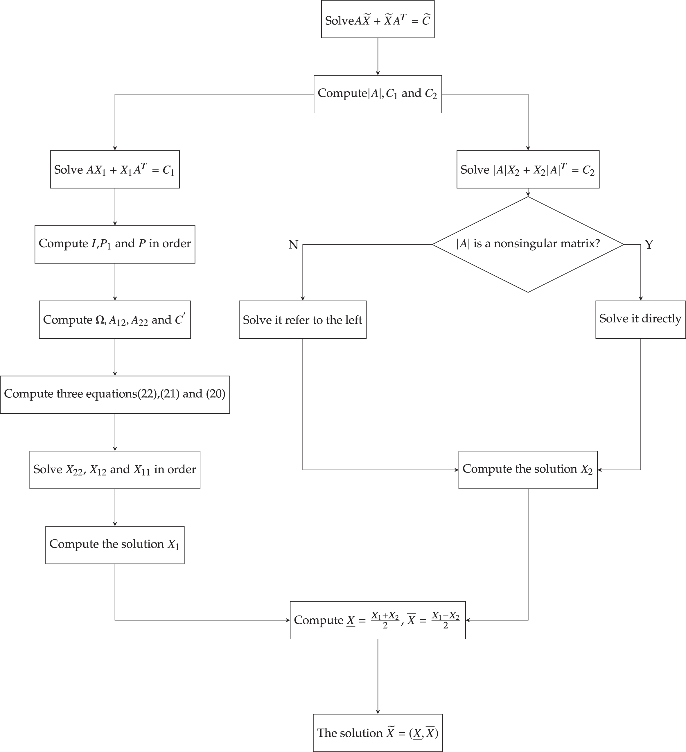
The Fig. 1 presents the process of solving the fuzzy matrix equation.

Fig. 1

The flow chart of solving the fuzzy singular Lyapunov matrix equation (2).

5 Examples

As a consequence of the discussion in the previous paragraph, we present four examples to illustrate the validate and the efficiency of our method. Two of them are small dimension examples. And one of them is singular consistent, the other one is singular inconsistent. The other two examples are large scale. All of the following examples are runned in the MATLAB (R2018b) environment. The hardware environment used in the experiment includes the system model of 90KSCTO1WW of Lenovo computer, the machine configuration is Intel(R) Core(TM) i5-10500 CPU@3.10GHz(12CPUs)

 3.1GHz, 16GB memory.

Example 1. Considering a fuzzy singular consistent Lyapunov matrix equation $A\tilde{X}+\tilde{X}{A}^T=\tilde{C},$ where $A=\left(\begin{array}{cccc}\hfill 2\hfill & \hfill -1\hfill & \hfill 2\hfill & \hfill 4\hfill \\ \hfill 4\hfill & \hfill -2\hfill & \hfill 5\hfill & \hfill 5\hfill \\ \hfill -10\hfill & \hfill 5\hfill & \hfill -12\hfill & \hfill -15\hfill \\ \hfill 8\hfill & \hfill -4\hfill & \hfill 10\hfill & \hfill 11\hfill \end{array}\right)$ with eigenvalues 0, i, - i, and -1,

and $\tilde{C}=({\tilde{C}}_1,{\tilde{C}}_2)$ , where ${\tilde{C}}_1=\left(\begin{array}{cc}\hfill (30+30r,84-24r)\hfill & \hfill (33+57r,126-36r)\hfill \\ \hfill (33+57r,126-36r)\hfill & \hfill (34+90r,166-42r)\hfill \\ \hfill (-191+76r,-20-95r)\hfill & \hfill (-207+91r,39-155r)\hfill \\ \hfill (66+75r,202-61r)\hfill & \hfill (58+117r,246-71r)\hfill \\ \hfill \hfill & \hfill \hfill \end{array}\right)$ and $\begin{array}{cc}\hfill & {\tilde{C}}_2=\hfill \\ \hfill & \left(\begin{array}{cc}\hfill (-191+76r,-20-95r)\hfill & \hfill (66+75r,202-61r)\hfill \\ \hfill (-207+91r,39-155r)\hfill & \hfill (58+117r,246-71r)\hfill \\ \hfill (-434+178r,-84-172r)\hfill & \hfill (-163+138r,107-132r)\hfill \\ \hfill (-163+138r,107-132r)\hfill & \hfill (98+96r,304-110r)\hfill \\ \hfill \hfill & \hfill \hfill \end{array}\right).\hfill \end{array}$

According to MNLS algorithm, we compute |A|, C₁ and C₂ as follows:

$\left|A\right|=A^{+}+A^{-}=\left(\begin{array}{cccc}\hfill 2\hfill & \hfill 1\hfill & \hfill 2\hfill & \hfill 4\hfill \\ \hfill 4\hfill & \hfill 2\hfill & \hfill 5\hfill & \hfill 5\hfill \\ \hfill 10\hfill & \hfill 5\hfill & \hfill 12\hfill & \hfill 15\hfill \\ \hfill 8\hfill & \hfill 4\hfill & \hfill 10\hfill & \hfill 11\hfill \end{array}\right),$ $\begin{array}{ccc}\hfill {\mathit{C}}_1& \hfill =\hfill & \underset{\_}{C}+\overline{C}\hfill \\ \hfill & \hfill =\hfill & \left(\begin{array}{cccc}114+6r& 159+21r& -211-19r& 268+14r\\ 159+21r& 200+48r& -168-64r& 304+46r\\ -211-19r& -168-64r& -518+6r& -56+6r\\ 268+14r& 304+46r& -56+6r& 402-14r\end{array}\right)\hfill \end{array}$ and $\begin{array}{ccc}\hfill & \hfill C_2\hfill & =\underset{\_}{C}-\overline{C}\hfill \\ \hfill & \hfill =\hfill & \left(\begin{array}{cccc}-54+54r& -93+93r& -171+171r& -136+136r\\ -93+93r& -132+132r& -246+246r& -188+188r\\ -171171r& -246+246r& -350+350r& -270+270r\\ -136+136r& -188+188r& -270+270r& -206+206r\end{array}\right).\hfill \end{array}$

Solving the original fuzzy equation is equivalent to solve the following two Lyapunov matrix equations $\begin{array}{cc}\hfill & {\mathit{AX}}_1+X_1{A}^T-C_1=0\mathit{and}\hfill \\ \hfill & \left|A\right|X_2+X_2|A{|}^T-C_2=0,\hfill \end{array}$ where |A| is semi-stable with one zero eigenvalue.

According to algorithm 1, we have the solutions and the residual norm of the two equations as the following, respectively: $\begin{array}{ccc}\hfill X_1& \hfill =\hfill & (\begin{array}{cc}\hfill 4.3037+0.2382r\hfill & \hfill 2.5501+0.8356r\hfill \\ \hfill 2.5501+0.8356r\hfill & \hfill -3.6260-0.8952r\hfill \\ \hfill 9.9809+1.4531r\hfill & \hfill 8.2548+1.8867r\hfill \\ \hfill 7.7452+0.1133r\hfill & \hfill 8.2548+1.8867r\hfill \\ \hfill \hfill & \hfill \hfill \end{array}\hfill \\ \hfill & \hfill \hfill & \begin{array}{cc}\hfill 9.9809+1.4531r\hfill & \hfill 7.7452+0.1133r\hfill \\ \hfill 8.2548+1.8867r\hfill & \hfill 8.2548+1.8867r\hfill \\ \hfill 8.2738+0.4336r\hfill & \hfill 6.7452-0.8867r\hfill \\ \hfill 6.7452-0.8867r\hfill & \hfill 9.5095+0.7734r\hfill \\ \hfill \hfill & \hfill \hfill \end{array}),\hfill \end{array}$ $\begin{array}{ccc}\hfill {\mathit{X}}_2& \hfill =\hfill & (\begin{array}{cc}\hfill -3.0400+3.0400r\hfill & \hfill -2.9200+2.9200r\hfill \\ \hfill -2.9200+2.9200r\hfill & \hfill -2.1600+2.1600r\hfill \\ \hfill -5.0000+5.0000r\hfill & \hfill -4.0000+4.0000r\hfill \\ \hfill -2.0000+2.0000r\hfill & \hfill -6.0000+6.0000r\hfill \\ \hfill \hfill & \hfill \hfill \end{array}\hfill \\ \hfill & \hfill \hfill & \begin{array}{cc}\hfill -5.0000+5.0000r\hfill & \hfill -2.0000+2.0000r\hfill \\ \hfill -4.0000+4.0000r\hfill & \hfill -6.0000+6.0000r\hfill \\ \hfill -5.0000+5.0000r\hfill & \hfill -3.0000+3.0000r\hfill \\ \hfill -3.0000+3.0000r\hfill & \hfill -3.0000+3.0000r\hfill \\ \hfill \hfill & \hfill \hfill \end{array}),\hfill \end{array}$ $\left|\right|R_1|{|}_F=1.7530e-12$ and $\left|\right|R_2|{|}_F=4.1236e-13.$

So the least norm fuzzy solution of the example is decided by $\begin{array}{ccc}\hfill \underset{\_}{X}& \hfill =\hfill & \frac{1}{2}(X_1+X_2)\hfill \\ \hfill & \hfill =\hfill & (\begin{array}{cc}\hfill 0.6318+1.6391r\hfill & \hfill -0.1850+1.8778r\hfill \\ \hfill -0.1850+1.8778r\hfill & \hfill -2.8930+0.6324r\hfill \\ \hfill 2.4905+3.2266r\hfill & \hfill 2.1274+2.9434r\hfill \\ \hfill 2.8726+1.0566r\hfill & \hfill 1.1274+3.9434r\hfill \end{array}\hfill \\ \hfill & \hfill \hfill & \begin{array}{cc}\hfill 2.4905+3.2266r\hfill & \hfill 2.8726+1.0566r\hfill \\ \hfill 2.1274+2.9434r\hfill & \hfill 1.1274+3.9434r\hfill \\ \hfill 1.6369+2.7168r\hfill & \hfill 1.8726+1.0566r\hfill \\ \hfill 1.8726+1.0566r\hfill & \hfill 3.2548+1.8867r\hfill \end{array})\hfill \end{array}$ and $\begin{array}{ccc}\hfill \overline{X}& \hfill =\hfill & \frac{1}{2}(X_1-X_2)\hfill \\ \hfill & \hfill =\hfill & (\begin{array}{cc}\hfill 3.6718-1.4009r\hfill & \hfill 2.7350-1.0422r\hfill \\ \hfill 2.7350-1.0422r\hfill & \hfill -0.7330-1.5276r\hfill \\ \hfill 7.4905-1.7734r\hfill & \hfill 6.1274-1.0566r\hfill \\ \hfill 4.8726-0.9434r\hfill & \hfill 7.1274-2.0566r\hfill \end{array}\hfill \\ \hfill & \hfill \hfill & \begin{array}{cc}\hfill 7.4905-1.7734r\hfill & \hfill 4.8726-0.9434r\hfill \\ \hfill 6.1274-1.0566r\hfill & \hfill 7.1274-2.0566r\hfill \\ \hfill 6.6369-2.2832r\hfill & \hfill 4.8726-1.9434r\hfill \\ \hfill 4.8726-1.9434r\hfill & \hfill 6.2548-1.1133r\hfill \end{array}).\hfill \end{array}$

Obviously, it shows $\overline{X}\ge \underset{\_}{X},r\in [0,1].$

Example 1 gives a specific process to solve a fuzzy singular consistent system with a zero eigenvalue and a pair of pure imaginary eigenvalues. It shows we can obtain its least norm fuzzy solution by using MNLS algorithm.

Example 2. Considering a fuzzy singular inconsistent Lyapunov matrix equation $A\tilde{X}+\tilde{X}{A}^T=\tilde{C},$ where $A=\left(\begin{array}{cccc}\hfill 0\hfill & \hfill -1\hfill & \hfill 2\hfill & \hfill 1\hfill \\ \hfill 1\hfill & \hfill 0\hfill & \hfill 4\hfill & \hfill 1\hfill \\ \hfill -2\hfill & \hfill -4\hfill & \hfill 0\hfill & \hfill -1\hfill \\ \hfill 0\hfill & \hfill 0\hfill & \hfill 0\hfill & \hfill -2\hfill \end{array}\right),$ its eigenvalues are 0, 4.5826i, - 4.5826i and -2, and $\tilde{C}=({\tilde{C}}_1,{\tilde{C}}_2)$ , where $\begin{array}{cc}\hfill & {\tilde{C}}_1=\hfill \\ \hfill & \left(\begin{array}{cc}\hfill (8+16r,38-14r)\hfill & \hfill (18+26r,59-15r)\hfill \\ \hfill (18+26r,59-15r)\hfill & \hfill (22+36r,72-14r)\hfill \\ \hfill (-27+15r,10-22r)\hfill & \hfill (-12+26r,36-22r)\hfill \\ \hfill (-10+8r,9-11r)\hfill & \hfill (11r,29-18r)\hfill \end{array}\right)\hfill \end{array}$ and $\begin{array}{cc}\hfill & {\tilde{C}}_2=\hfill \\ \hfill & \left(\begin{array}{cc}\hfill (-27+15r,10-22r)\hfill & \hfill (-10+8r,9-11r)\hfill \\ \hfill (-12+26r,36-22r)\hfill & \hfill (11r,29-18r)\hfill \\ \hfill (-76+18r,-18-40r)\hfill & \hfill (-45+16r,-8-21r)\hfill \\ \hfill (-45+16r,-8-21r)\hfill & \hfill (-6+6r,6-6r)\hfill \end{array}\right).\hfill \end{array}$

According to MNLS algorithm, we compute |A|, C₁ and C₂ as follows: $\left|A\right|=A^{+}+A^{-}=\left(\begin{array}{cccc}\hfill 0\hfill & \hfill 1\hfill & \hfill 2\hfill & \hfill 1\hfill \\ \hfill 1\hfill & \hfill 0\hfill & \hfill 4\hfill & \hfill 1\hfill \\ \hfill 2\hfill & \hfill 4\hfill & \hfill 0\hfill & \hfill 1\hfill \\ \hfill 0\hfill & \hfill 0\hfill & \hfill 0\hfill & \hfill 2\hfill \end{array}\right),$ $\begin{array}{cc}\hfill & C_1=\underset{\_}{C}+\overline{C}=\hfill \\ \hfill & \left(\begin{array}{cccc}46+2r& 77+11r& -17-7r& -1-3r\\ 77+11r& 94+22r& 24+4r& 29-7r\\ -17-7r& 24+4r& -94-22r& -53-5r\\ -1-3r& 29-7r& -53-5r& 0\end{array}\right)\hfill \end{array}$ and $\begin{array}{cc}\hfill & C_2=\underset{\_}{C}-\overline{C}\hfill \\ \hfill & =\left(\begin{array}{cccc}-30+30r& -41+41r& -37+37r& -19+19r\\ -41+41r& -50+50r& -48+48r& -29+29r\\ -37+37r& -48+48r& -58+58r& -37+37r\\ -19+19r& -29+29r& -37+37r& -12+12r\end{array}\right).\hfill \end{array}$

According to the extension method, we need to solve the following two equations $\begin{array}{cc}\hfill & {\mathit{AX}}_1+X_1{A}^T-C_1=0\mathit{and}\left|A\right|X_2+X_2|A{|}^T\hfill \\ \hfill & -C_2=0,\hfill \end{array}$ where |A| is non-singular.

According to algorithm 1, after minus the inconsistent part, we obtain the solution of the singular consistent Lyapunov matrix equation and the residual norm is 7.7499e - 14. Moreover, we also can obtain the result that both the norm of AX₁ + X₁A ^T  - C₁ and $\mathcal{I}$ are 2.8829. So the numerical solutions of the two equations as the following, respectively: $\begin{array}{ccc}\hfill X_1& \hfill =\hfill & (\begin{array}{cc}\hfill 8.3535+1.3263r\hfill & \hfill 7.1279+1.5666r\hfill \\ \hfill 7.1279+1.5666r\hfill & \hfill 7.6087+1.1832r\hfill \\ \hfill 11.7261+1.3569r\hfill & \hfill 8.2853+1.8936r\hfill \\ \hfill 6.2924-0.1897r\hfill & \hfill 5.9265+1.7696r\hfill \end{array}\hfill \\ \hfill & \hfill \hfill & \begin{array}{cc}\hfill 11.7261+1.3569r\hfill & \hfill 6.2924-0.1897r\hfill \\ \hfill 8.2853+1.8936r\hfill & \hfill 5.9265+1.7696r\hfill \\ \hfill 10.6236+2.3920r\hfill & \hfill 8.6840-0.8129r\hfill \\ \hfill 8.6840-0.8129r\hfill & \hfill 0.0570+0.0063r\hfill \end{array})\hfill \end{array}$ and $X_2=\left(\begin{array}{cccc}-3+3r& -3+3r& -5+5r& -2+2r\\ -3+3r& -2+2r& -4+4r& -6+6r\\ -5+5r& -4+4r& -5+5r& -3+3r\\ -2+2r& -6+6r& -3+3r& -3+3r\\ \end{array}\right).$

So the least norm fuzzy solution of the example is decided by

$\begin{array}{ccc}\hfill \underset{\_}{X}& \hfill =\hfill & \frac{1}{2}(X_1+X_2)\hfill \\ \hfill & \hfill =\hfill & (\begin{array}{cc}\hfill 2.6768+2.1632r\hfill & \hfill 2.0640+2.2833r\hfill \\ \hfill 2.0640+2.2833r\hfill & \hfill 2.8043+1.5916r\hfill \\ \hfill 3.3631+3.1784r\hfill & \hfill 2.1427+2.9468r\hfill \\ \hfill 2.1462+0.9051r\hfill & \hfill -0.0367+3.8848r\hfill \end{array}\hfill \\ \hfill & \hfill \hfill & \begin{array}{cc}\hfill 3.3631+3.1784r\hfill & \hfill 2.1462+0.9051r\hfill \\ \hfill 2.1427+2.9468r\hfill & \hfill -0.0367+3.8848r\hfill \\ \hfill 2.8118+3.6960r\hfill & \hfill 2.8420+1.0936r\hfill \\ \hfill 2.8420+1.0936r\hfill & \hfill -1.4715+1.5032r\hfill \end{array})\hfill \end{array}$ and $\begin{array}{ccc}\hfill \overline{X}& \hfill =\hfill & \frac{1}{2}(X_1-X_2)\hfill \\ \hfill & \hfill =\hfill & (\begin{array}{cc}\hfill 5.6768-0.8368r\hfill & \hfill 5.0640-0.7167r\hfill \\ \hfill 5.0640-0.7167r\hfill & \hfill 4.8043-0.4084r\hfill \\ \hfill 8.3631-1.8216r\hfill & \hfill 6.1427-1.0532r\hfill \\ \hfill 4.1462-1.0949r\hfill & \hfill 5.9633-2.1152r\hfill \end{array}\hfill \\ \hfill & \hfill \hfill & \begin{array}{cc}\hfill 8.3631-1.8216r\hfill & \hfill 4.1462-1.0949r\hfill \\ \hfill 6.1427-1.0532r\hfill & \hfill 5.9633-2.1152r\hfill \\ \hfill 7.8118-1.3040r\hfill & \hfill 5.8420-1.9064r\hfill \\ \hfill 5.8420-1.9064r\hfill & \hfill 1.5285-1.4968r\hfill \end{array}).\hfill \end{array}$

Obviously, it shows $\overline{X}\ge \underset{\_}{X},r\in [0,1].$

Example 2 presents a specific process to solve a fuzzy singular inconsistent Lyaunov matrix equation with a zero eigenvalue and a pair of pure imaginary eigenvalues. This example is more difficult than example 1 because it need to compute the inconsistent part.

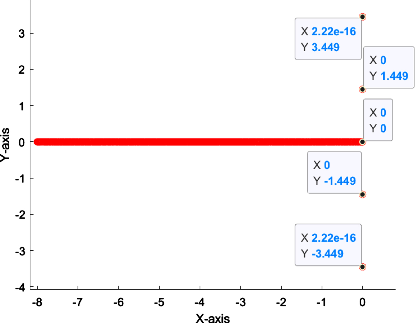
Example 3. We consider a fuzzy singular Lyapunov matrix equation, where A and $\tilde{C}$ are construced by the following steps:

$\Sigma =\left(\begin{array}{ccccc}0& 1& -1& 1& 0\\ -1& 0& -1& -1& 0\\ 1& 1& 0& -3& 0\\ -1& 1& 3& 0& 0\\ 0& 0& 0& 0& 0\end{array}\right)$ is a 5 × 5 matrix with eigenvalues 1.4495i, - 1.4495i, 3.4495i, - 3.4495i.

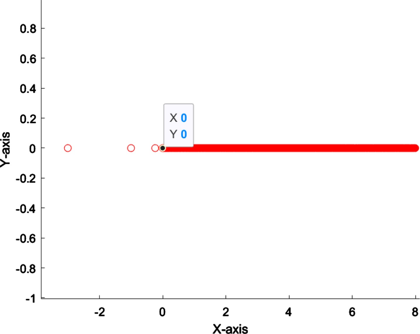
$\Delta =\left(\begin{array}{cccccc}-4& 1& & & & \\ 1& -4& 1& & & \\ & 1& -4& \ddots & & \\ & & \ddots & \ddots & \ddots & \\ & & & \ddots & -4& 1\\ & & & & 1& -4\end{array}\right)$ is a n × n tri-diagonal matrix whose diagonal entries are -4, whose entries above diagonal and below diagonal are both 1.

$A=\left(\begin{array}{cc}\Delta & \\ & \Sigma \end{array}\right)$ is a (n + 5) × (n + 5) square matrix.

Let $\underset{\_}{Y}=T_1+T_{2}r$ and $\overline{Y}=T_3-(T_3-T_1-T_2)r$ , where T₁ and T₂ is a random symmetric matrix with elements in [0, 5], T₃ is a random symetric matrix with elements in [10, 20].

$Y_1=\underset{\_}{Y}+\overline{Y}$ and $Y_2=\underset{\_}{Y}-\overline{Y}$ .

C₁ = AY₁ + Y₁A ^T and C₂ = |A|Y₂ + Y₂|A| ^T .

$\underset{\_}{C}=\frac{1}{2}(C_1+C_2)$ and $\overline{C}=\frac{1}{2}(C_1-C_2)$

Construt $\tilde{C}=(\underset{\_}{C},\overline{C})$ .

We present condition numbers of A and |A| in the Table 1. By the table, we can see A and |A| having almost the same condition numbers, and the condition numbers of A and |A| increase as n increases.

Table 1

The condition numbers versus n

n	The condition	The condition
	numbers of A	numbers of |A|
100	48.3742	48.3742
400	178.064	178.064
900	388.812	388.812
1600	680.617	680.617
2500	1053.48	1053.48
3600	1507.40	1507.40

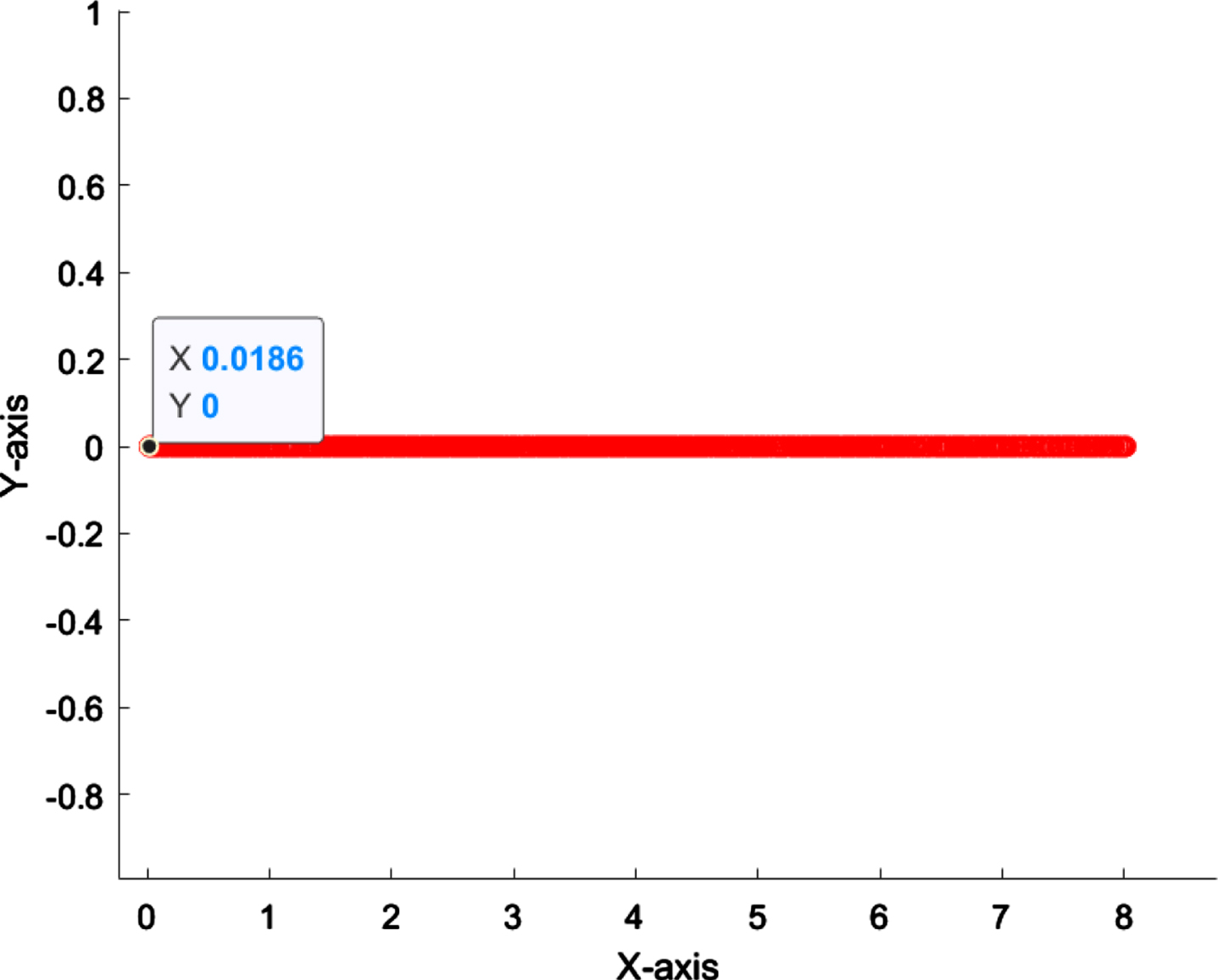
Table 2 presents the residual norm and CPU running time of solving matrix equations (16), (17) when n takes different values. By this table, solving (16) costs more time, because more eigenvalues of A close to zero. Please see Figs. 2 and 3 . We also find the kronecker method fails to solve this example when n ≥ 100 .

Fig. 2

The spectral distribution of A (n = 3600).

Fig. 3

The spectral distribution of |A| (n = 3600).

Table 2

Numerical results when n takes different values

n	||R1|| F	||R2|| F	(16) CPU time	(17) CPU time	The kronecker method
2	1.0380e-12	3.8878e-12	0.0037	0.0032	it costs 39 seconds and the residual norm is 3.3270e-11
3	2.4711e-12	6.3108e-12	0.0065	0.0067	it costs 1345 seconds and the residual norm is 7.4788e-10
100	5.4663e-11	7.2947e-11	0.3376	0.1861	it costs more than 1 hour and the residual norm is 5.7833e-09
400	3.6801e-10	4.1428e-10	4.6810	2.6938	out of memory
900	1.1522e-09	1.0449e-09	22.1239	12.4884	out of memory
1600	2.3946e-09	2.2830e-09	72.6816	41.7671	out of memory
2500	4.8409e-09	3.2166e-09	197.6176	145.3564	out of memory
3600	8.5196e-09	5.8851e-09	631.3729	346.6931	out of memory

The above numerical experiments can be implemented in parallel, so the total time for solving the fuzzy equation (2) is the CPU time for solving the equation (16).

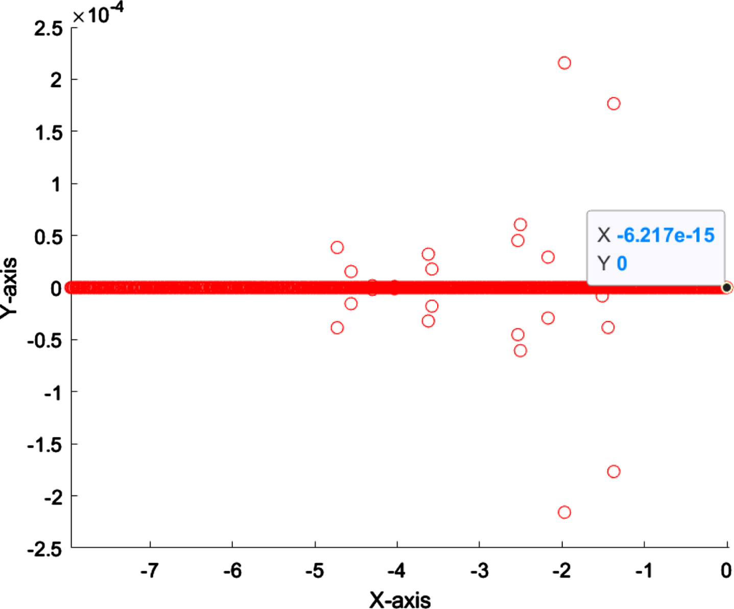
Example 4. Considering a fuzzy singular inconsistent Lyapunov matrix equation $A\tilde{X}+\tilde{X}{A}^T=\tilde{C}$ , where A and $\tilde{C}$ are constructed according to following steps:

We discretize $-\Delta u+\overrightarrow{a}\nabla u$ with Neumann boundary conditions to obtain the matrix A by using the finite element method with triangular elements and quadratic basis ([10]). It is well-known that A is semi-stable and dim $\left(\mathcal{N}\right(A\left)\right)$ =1. In this experiment, we chose A with n = 2601 and $\overrightarrow{a}=1$ in 1D.

Construct $\tilde{C}=(\underset{\_}{C},\overline{C})$ , where $\underset{\_}{C}=(T_1-T_3)+(T_2-T_4)r,$ $\overline{C}=-(T_1+T_2)-(T_3+T_4)r,$ where T₁ and T₂ are random symmetric matrices with elements in [5, 10], T₃ and T₄ are random symetric matrices with their elements in [0, 5].

The condition numbers of A and |A| are 2108.03 and 430.812, respectively. Figure 4 and 5 are the spectral distributions of A and |A|, respectively.

Fig. 4

The spectral distribution of A.

Fig. 5

The spectral distribution of |A|.

According to the spectral distribution of |A| shown above, we know |A| is a non-singular matrix. Tables 3 and 4 presents the numerical results of (16) and (17), respectively. The condition numbers of A and |A| are 2108.03 and 430.812, respectively.

Table 3

The numerical result of solving the matrix equation (16)

Number	||AX1 + X1A T  - C|| F	(16)CPU time	$\left|\right|\mathcal{I}|{|}_F$	||AX1 + X1A T  - C1|| F	The kronecker method
1	2.5051e-09	248.7264	0.0010	0.0010	out of memory
2	2.5064e-09	206.1042	0.1089	0.1089	out of memory
3	2.5090e-09	207.7534	1.2563	1.2563	out of memory
4	4.0535e-09	224.9970	76.1134	76.1134	out of memory
5	6.0800e-09	208.7395	158.6147	158.6147	out of memory
6	1.4313e-08	215.7241	924.3292	924.3292	out of memory

Table 4

The numerical result of solving the matrix equation (17)

Number	||R2|| F	(17)CPU time
1	1.3315e-08	37.1101
2	1.3159e-08	36.5623
3	1.3159e-08	37.0265
4	1.3329e-08	36.4116
5	1.3387e-08	35.4866
6	1.3316e-08	40.2629

By these two tables, we find (17) is solved more easily than (16). The reason is the nonsingularity of |A|. Obviously, we implement algorithms parallel.

Example 4 solves a fuzzy singular inconsistent Lyapunov matrix equation with a zero eigenvalue. The fourth and fifth columns in Table 3 are almost equal illustrates that the result we obtained is the least squares solution of it. We also try to solve the fuzzy and singular inconsistent Lyapunov matrix equation by using Kronecker product directly. Clearly, we get the trouble of out of memory.

6 Conclusion

The main contribution of this paper is to propose an appropirate approach to solve FSLME which has never been solved efficiently. The approach combines the extension method in [20] with the method to solve singular crisp Lyapunov matrix equations in [11]. Examples in this paper show the validate and the efficiency of this approach.