
Abstract
In agriculture, selecting an “appropriate plant for an appropriate soil” is a crucial stage for all sorts of lands. There are different types of soil found in India. It is necessary to understand the features of the soil type to predict the types of crops cultivated in a particular soil. This leads to significant inconsistencies and errors in large-scale soil mapping. However, manually analyzing the soil type in the laboratory is cost-effective and time-consuming, yet it produces an inaccurate classification result. To overcome these challenges, a novel AQU-FRC Net (Aquila – Faster Regional Convolutional Neural Neural) is proposed for the automatic prediction of soil and recommending suitable crops based on a soil-crop relationship database. The soil images were pre-processed using a Scalable Range-based Adaptive Bilateral Filter (SCRAB) for eliminating the noise artifacts from the images. The pre-processed images were classified using Faster-RCNN, which utilized MobileNet as a feature extraction network. The classification results were optimized by the Aquila optimization (AQU) algorithm that normalizes the parameters of the network to achieve better results. The proposed AQU-FRC Net achieves a high accuracy of 98.16% for predicting soil. The experimental results demonstrate that the model successfully predicts the soil when compared to other meta-heuristic-based methods.
Introduction
Agriculture is the primary source of economic development and has a large impact on Gross Domestic Product (GDP). Nowadays the demand for agriculture and crop cultivation is decreasing due to inadequate rainfall, climatic condition, and improper maintenance of land [1]. Toward the end of 2050, the population will increase by 9.1 billion in the world [2]. As the population increases the demand for the production of food is also increasing. The United Nations (UN) Food and Agricultural Organization (FAO) estimates that food production necessities to increase by nearly 70% to feed this growing population [3]. So agricultural cultivation also needs to be increased. To meet the increasing demands, farmers must apply toxic pesticides more frequently and also apply higher pressure on the soil [4]. As a result, agriculture is significantly impacted, and the land eventually becomes unproductive and dry.
To increase cultivation of the crop, soil classification is one of the primary aspects to decide what kind of crops can grow. Soil is a dynamic living resource, that promotes crop yields as well as ecological processes. [5, 6]. The physical and chemical characteristics of soil change throughout time due to several influences, including changes in both locations and time [7]. There are two ways to determine the type of soil such as image analysis and chemical analysis. The chemical analysis is often carried out in a laboratory using several chemicals which is expensive, not environment-friendly [8], time-consuming, and complex to access for the common farmers. Meanwhile, image processing identifies soil based on its color and texture. Additionally, several classifiers, such as Artificial Neural Network (ANN), Support Vector Machine (SVM), and Decision Trees (DT), are employed for classification. Deep learning (DL) is now often used in many applications, including object detection [9]. For agricultural applications like plant diagnosis, disease detection, etc., Convolution Neural Networks (CNN) in particular attracted a lot of attention in deep learning.
The early identification and selection of soil types is the first step before beginning crop cultivation. Because “not all sort of soil is suited for all kind of crop” and each soil has its own unique set of characteristics and harvesting ability for agricultural development in diverse ways [10]. To analyze this issue, an efficient architecture named AQU-FRC Net, in which MobileNet is integrated with Faster R-CNN was developed. The main objective of the proposed framework is as follows, The primary purpose of this work is to present a novel AQU-FRC Net (Aquila – Faster RCNN) for the automatic prediction of soil type and recommending suitable crops based on the soil-crop relationship database An integration of Mobilenet with Faster R-CNN is used for real-time soil prediction. The proposed Faster RCNN is used to classify the soils into black soil, red soil, alluvial soil, yellow soil, sandy loam soil, and peat soil. Aquila optimization is applied to the Faster RCNN for normalizing the appropriate parameters to attain better classification results. The efficiency of the proposed methodology is analyzed using the metrics like accuracy, recall, specificity, precision, and F1-score.
The remaining section of this paper is arranged as follows; section 2 explains the Literature survey. Section 3 includes the proposed model of AQU-FRC Net. Section 4 comprises the result and discussion of the proposed method. Section 5 holds closing remarks and future enhancements.
Literature survey
In recent years, many Machine Learning (ML) and DL studies for various soil predictions based on pH value, nutrients, and soil moisture strategies have been discussed by researchers. This section provides a brief overview of some of the most recent studies.
In 2022 Motwani, A., et al. [11] developed a CNN and Random Forest (RF) Algorithm for the examination of soil and crop detection. In soil analysis, the soil image from Soil Classification Image Dataset is converted into pixels and further classifies the image using CNN. In the crop prediction process, the Crop Prediction in India dataset is preprocessed and encoded using hot encoding, then the RF algorithm uses bagging to select sample data. Herein crop prediction has a limited amount of data.
In 2022 Uddin, M. and Hassan, M., [12] developed a soil prediction technique using a feature-based algorithm. The soil categorization is based on frequent φ-Pixels, quartile histogram-oriented gradients, and a feature selection method. To evaluate the performance of selected features four machine learning algorithm is utilized. But this method fails to analyze the grass in the predicted soil.
In 2022 Lanjewar, M.G et al., [13] presented a CNN-based soil images classification. The dataset was subjected to the image augmentation process, and the models were subsequently trained using these augmented images. Pre-trained weights used in the TensorFlow and Keras DL algorithms accurately classify soil images. The suggested model was examined using the K-fold method.
In 2021 Kumar, S., et al., [14] presented a Chaotic Spider Monkey Optimization (CSMO) algorithm and a bag of features for soil detection. The surf method is used for feature extraction. The CSMO approach exhibits desirable efficiency and enhanced global search capability and is used to cluster the key points for soil detection.
In 2021 Dash, R., et al., [15] presented an ML technique for the categorization of crops. The parameters like micronutrients, macronutrients of soil, and climatic conditions like sunlight, rain, temperature, humidity, and pH of soil are considered and classified using SVM and DT. The model attains 92% of accuracy, yet SVM needed more training samples.
In 2021 Agarwal, R., et al., [16] presented chaotic Henry’s Gas Solubility Optimization (HGSO) for soil image classification. The soil images are categorized using an ideal bag-of-features-based automated soil prediction approach, and the ideal visual words are generated using an improved HGSO. The HGSO model provides better convergence precision.
In 2021 Barkataki, N, et al., [17] developed a DL-based soil classification from Ground Penetrating Radar (GPR) B scans. To train and validate the suggested CNN model, a synthetic dataset is created using GPRMax. Based on the suggested model, soil types can be automatically classified and GPR systems can be calibrated based on best penetration depths and minimum noise levels.
In 2020 Ghazali, M.F., et al., [18] put forward a soil analysis based on soil salinity and moisture index. To validate the test the Landsat 8 satellite images were used in soil feature analysis. The test was conducted in dry soil and a paddy farm. Soil pH is achieving an accuracy of (2– 7.59). Herein, the spectral and spatial resolution of Landsat 8 satellite images is relatively low.
In 2020 Suchithra, M.S. and Pai, M.L., [19] developed an Extreme Learning Machine (ELM) for soil nutrient classification. The soil characteristics were examined, including soil pH, phosphorus, potassium, carbon, and boron soil fertility indices at the village level. various activation functions were used by ELM to classify the data. The model achieves an accuracy of above 80%.
In 2019 Padarian, J., et al., [20] deployed a CNN model for soil properties prediction in regional spectral data. The soil properties like CEC, OC, clay, pH, sand, and N are utilized. The LUCAS soil database is used in validation. To fully utilize the CNN model, a 2-dimensional spectrogram displays reflectance as a function of wavelength and frequency. However, the multi-task CNN was ineffective on a smaller dataset.
In 2019 de Oliveira Morais, P.A., et al., [21] presented soil texture prediction using digital image processing. Clay and sand contents were defined by the pipette method. Using PLS2 multivariate regression, particle contents in the given size fractions were related to image data. Multivariate statistics from the sampling and validation dataset were assessed via bootstrapping analysis. The model is eco-friendly and does not use any chemical agents.
In 2018 Rahman, S.A.Z., et al., [22] developed an ML algorithm for soil predicting and providing recommendations for a crop’s production on that particular soil. soil parameters such as pH, salinity, zinc, boron, and calcium are used in soil prediction. The ML algorithms such as Bagged Trees, weighted k-Nearest Neighbor, and Gaussian kernel-based SVM are utilized in classification whereas SVM yields higher accuracy of 94.95%.
From the related studies, various ML and DL techniques were used for soil prediction based on moisture, pH value, and soil nutrients. The accuracy rate of the aforementioned methods is low with the use of datasets. In our proposed model the real-time images are used to improve the accuracy level. The proposed AQU-FRCNet focused on soil prediction and crop recommendation based on soil types. The Faster R-CNN is used in the classification phase and predicts the soil types. The AQU algorithm is used to normalize the parameters to attain higher accuracy in classification results. Table 1 shows the Comparative analysis with existing techniques.
Comparative analysis with existing techniques
Comparative analysis with existing techniques
Soil is a natural body made up of different layers and different components. Soils are recognized by their physical features such as texture, color, and landscape region. The target of the proposed work is to predict the soil types and recommendation of crops based on based soil types. In this section, the soil prediction is based on three phases: Data collection, data preprocessing, and data classification. A flow diagram of the proposed soil prediction model is shown in Fig. 1.
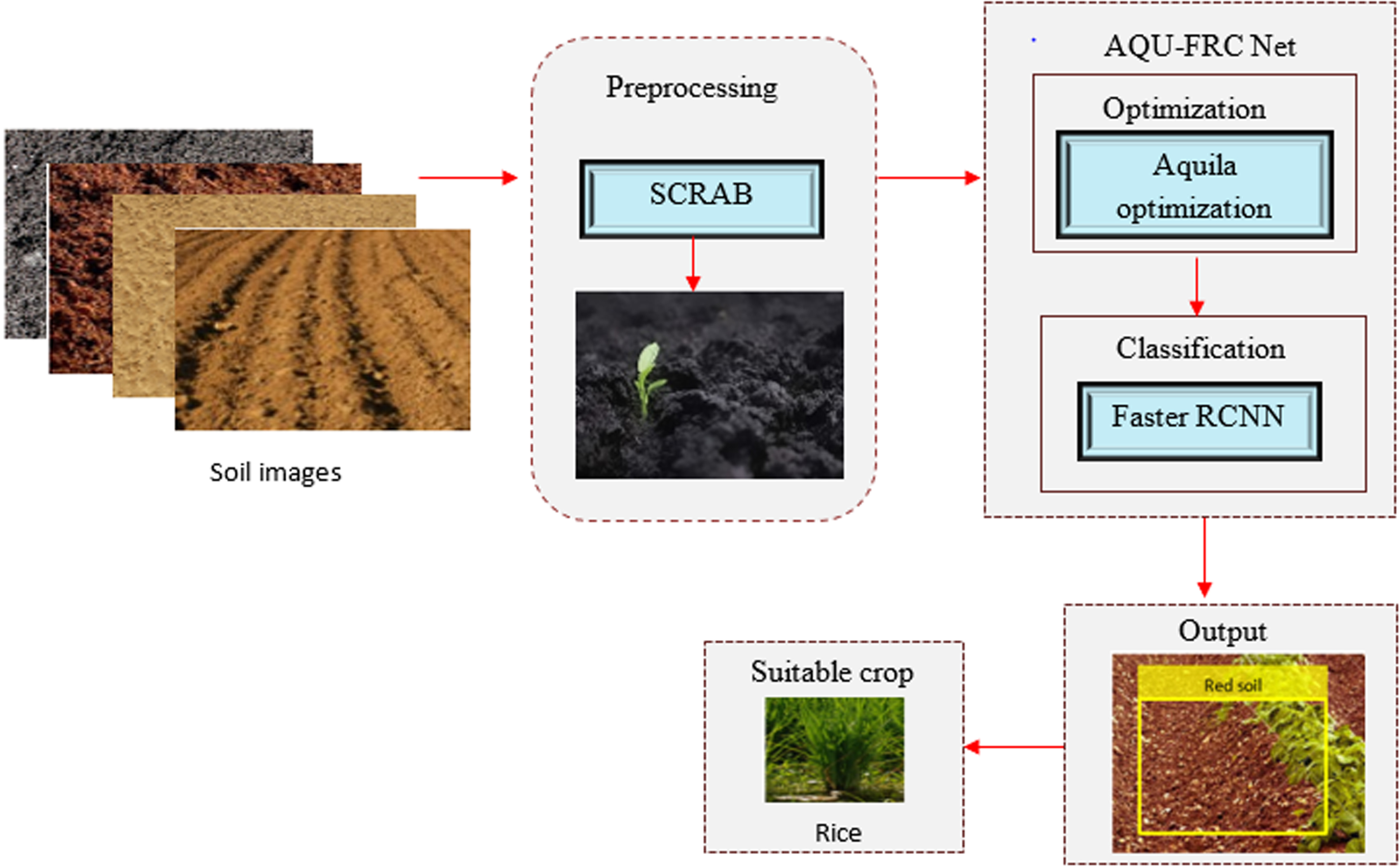
Flow diagram of the proposed soil prediction method.
Our database contains images of six different types of soil (yellow soil, alluvial soil, peat soil, red soil, black soil, and sandy loam soil). Using camera devices, the soil images with various resolutions were collected under serval conditions depending on the season (temperature, humidity) and different Agri fields. For that purpose, serval Agri lands have been visited in Tirunelveli, Kanyakumari, Thoothukudi, and Assam. Figure 2 depicts some of the sample soil images.
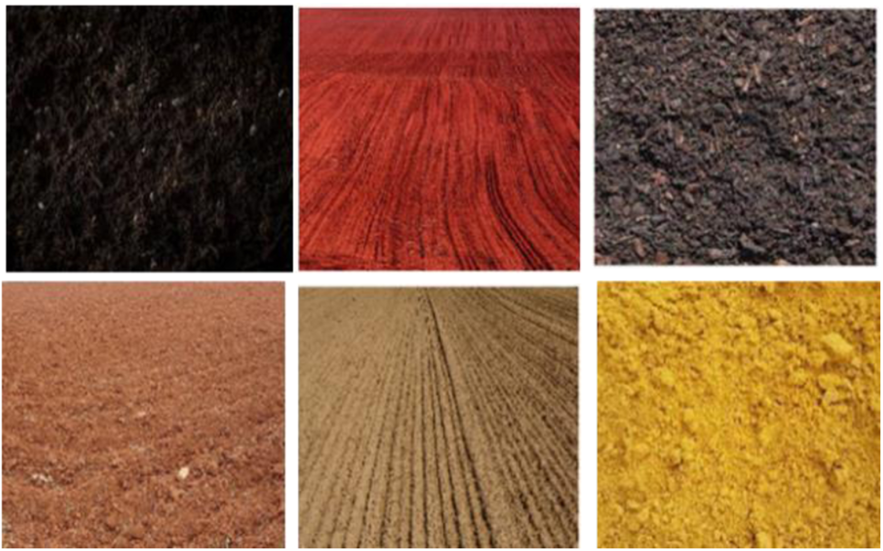
Sample soil images of different categories.
Pre-processing is a technique used to improve specific aspects and remove unwanted distortions from input images. Herein the scalable range-based adaptive bilateral filter (SCRAB) is utilized for preprocessing. SCRAB is a smoothening, noise-reducing, non-linear, and edge-preserving filter. The Gaussian distribution function first determines the intensity pixel value and the weighted intensity mean of each surrounding pixel. The range weight is then determined using Euclidean distances and radiometric differences. By applying this parameter, the noise is significantly decreased but the edges of the image pixels are retained.
Bilateral filtering b(x) for an image is defined in Equation (1).
After normalization
In noisy images, edge variations are not gathered completely, which is considered to be one of the major weaknesses of the bilateral filter. Herein, SCRAB filter is used to fix this defect and it is derived as,
Where Ω y refers to the pixel set of (2n + 1) * (2n + 1) pixel window where n = 2. The positive parameters are n and k, Ω y is the average value; p is a stable variable and v (x) is a range-based function. The three parameters used to control s r are the scaling factor σ r , the linear constant coefficients n = 2andk = 1. σ r ensures the elevated rate for photometric resemblance among x central pixel x and its m adjacent. Samples of before preprocessing and after preprocessing are shown in Fig. 3.
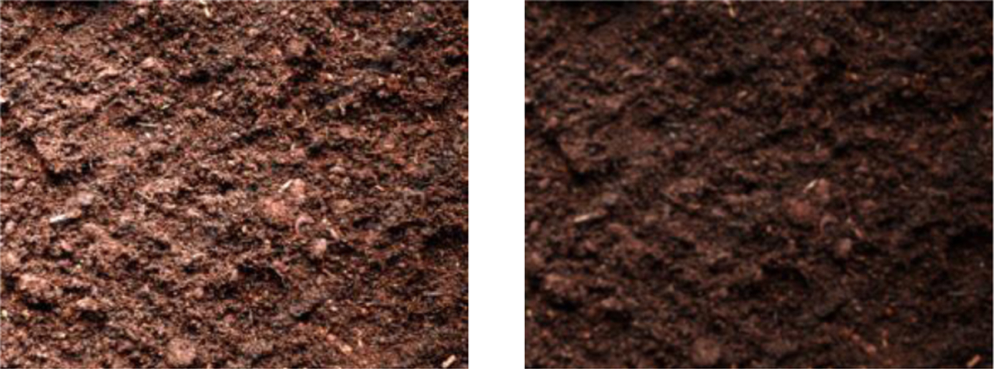
Samples of before-preprocessing and after preprocessing.
The proposed AQU-FRC Net focuses on the prediction of soil types. The structure of the proposed AQU-FRC Net was illustrated in Fig. 4. The proposed model includes three phases that include feature extraction, classification, and optimization. Faster R-CNN is involved in the first two phases and the Aquila optimization algorithm is used for normalizing the parameters to obtain optimal results.
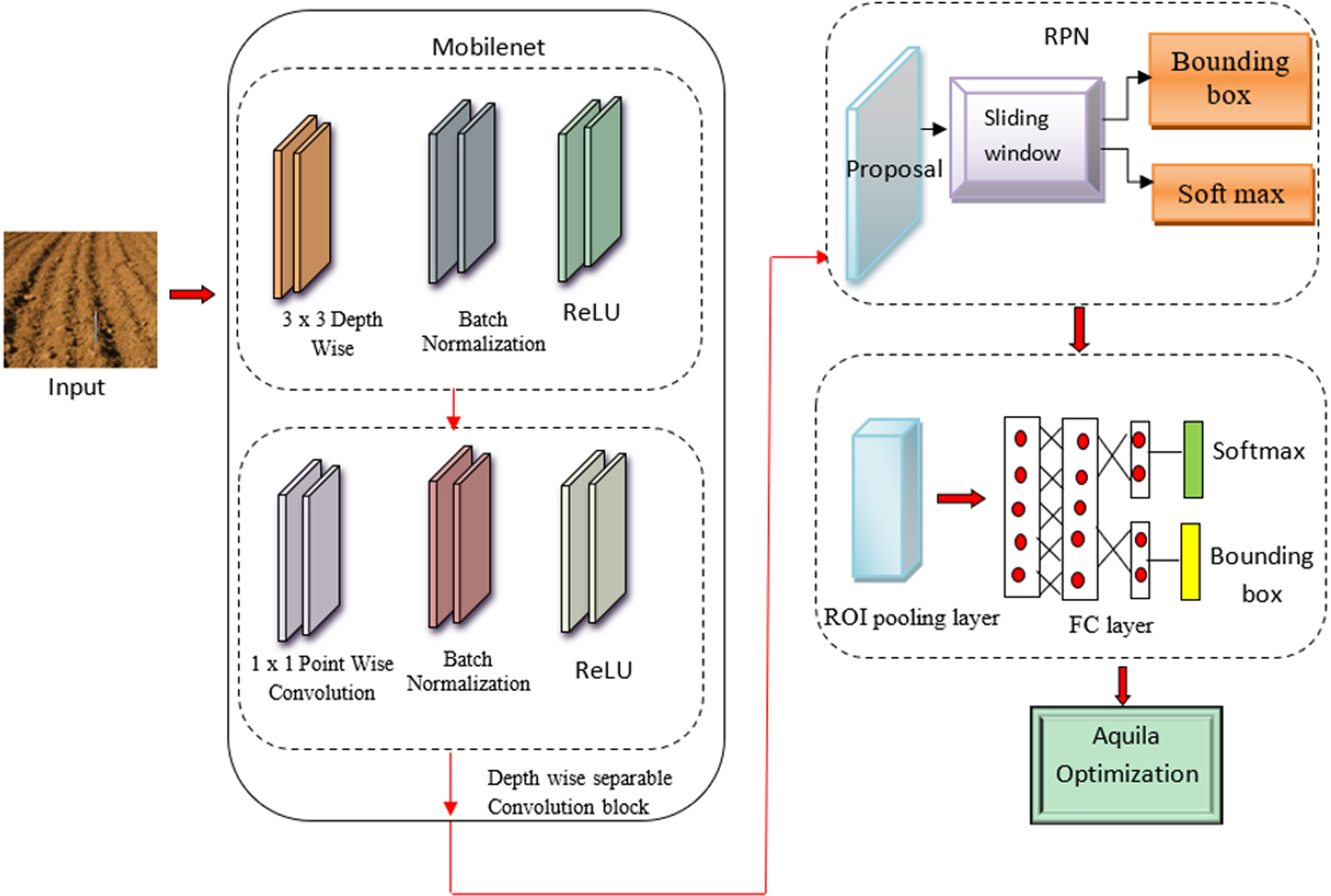
Architecture of AQU-FRC Net Network.
For detecting the soil parameters Faster RCNN is proposed that employed a new MobileNet for precise detection. For object identification applications that rely on region proposal methods to forecast the positions, a faster RCNN is used. Using Faster R-CNN shares full soil image convolutional characteristics with fast RCNN, making region prediction nearly free. Even though these bounding boxes are not precise, they can still be analysed by pooling regions of interest (RoI). When RoI pooling is done for each region, the most accurate bounding box coordinates can be determined.
MobileNet
MobileNet is used as a feature pyramid network for the input images for feature extraction. The lightweight deep convolutional neural network known as MobileNet is substantially smaller and performs considerably faster. The purpose of the MobileNet layers is to convert the pixels from the preprocessed image into features that characterize the information and transmit these to the preceding layers. Depth-wise separate convolutions filter the input data by applying a single filter to each input, followed by a 1×1 convolution layer aggregate these filters into a set of output features. The last fully connected layer feeds into a softmax layer without nonlinearity, so all layers have batch norms and ReLUs. MobileNet has 28 layers if depthwise and pointwise convolutions are excluded.
Regional proposal network
The Regional Proposal Network (RPN) is a fully convolutional network that provides region proposals and can predict object boundaries and scores at every point concurrently. It accepts the feature map as input produced by the last convolutional layer of MobileNet. Using an input image of any size, an RPN provides a set of rectangular object proposals along with corresponding object scores. A reference anchor box with n×n initializations is created by RPN. Each reference anchor box has its scale and aspect ratio for each conv feature map location. The anchor box is formatted as a rectangle box and chosen with an intersection over union relationship between the anchor box and ground truth box. An anchor with a sliding window focus is connected to scales and aspect ratios. A sliding window is converted into a low-dimensional vector that is then fed into two fully interconnected neighborhood layers. In Faster R-CNN, an objective function reduces the multi-task loss using Mobilenet, and the loss function is derived from Equation (5).
Where i depicts the anchor index.
The input feature maps and proposals can be collected through the roi pooling layer. The argmax switches are utilized by the reverse function of the ROI pooling layer to assess the partial derivative of the loss function concerning each input variable s
m
.
Where, every mini-batch ROI and output unit t
qn
, the partial derivative
Where the filter bank is denoted as k, the image tensor input is denoted as q, the filter number is denoted as f, z indicates the number of layers, a filter number is denoted as N, a and b indicate the spatial coordinates and r denotes the convolution output.
A function was estimated for the object identification method using equation (8)
the log loss is defined from two classes such as object vs not object. The
An AQU algorithm generally mimics the social behavior of Aquila to capture its prey. It is the population-based optimization algorithm, that is the same as other metaheuristics, which initiates with an initialized population of N agents. The agents in the existing population are upgraded until they find the best solution based on the best agent and the AQU. Equation (10) is used to generate the initial population m that is composed of N solutions.
In Equation (10), ikn and jkn signify the limits of search space. s1 ∈ [0, 1] denotes a random value and Dim is the dimension of the agent. As a next step in the AQU technique, either exploration or exploitation will be conducted until the best solution can be found. In the exploration, the best agent (Na) and the average of the agents (Nb) are used, and its mathematical formulation is provided as:
The search during the exploration phase is controlled by
The random values are denoted by u and v in Equation (10), where d = 0.01 and = 1.5. Additionally, H1 refers to the movements used to monitor the best individual solution, as shown in the equation below:
Different varieties of crops are grown in different sorts of areas and soils. A conventionally placed object exists in each space, which could be called common sense. For instance, based on human perception crops like sugarcane, turmeric, wheat, banana, etc. can grow in alluvial soil. Similarly, potatoes, rice, maize, and sugarcane can grow in yellow soil. Furthermore, crops like ladies’ fingers can suit all soil series, and sugarcane can suit alluvial soil and yellow soil. The crop cultivation in these spaces varies according to climatic conditions and many other factors. Generally, this part can be adjusted appropriately according to the specific situations. The names of the spaces and the objects are termed as “soil– crop relationship database” which was developed and shown in Fig. 5. After predicting the soil types, the suitable crops for that soil series for the given map were suggested based on the soil-crop relationship database.
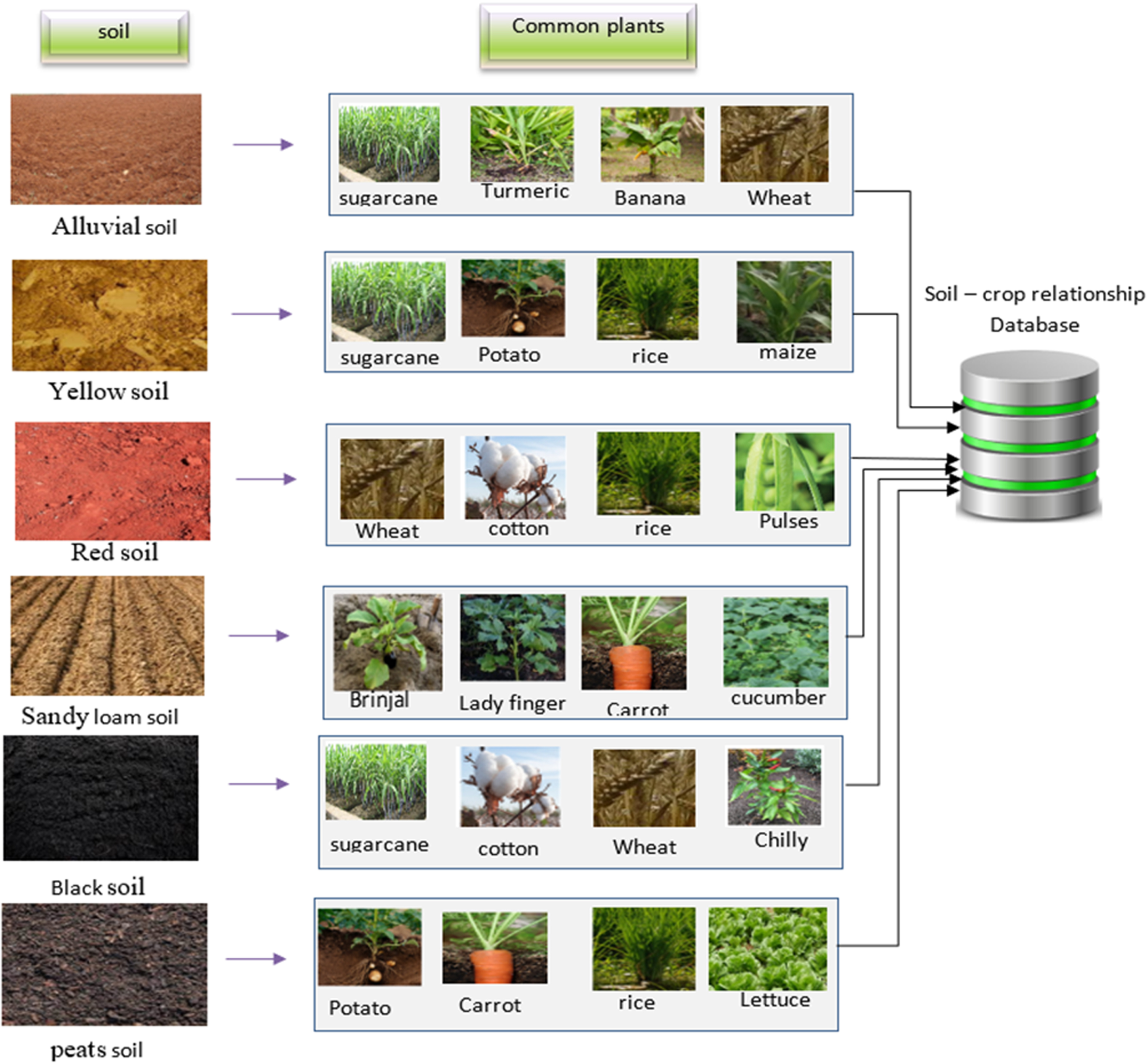
Soil - Crop relationship database.
In the proposed work, architecture is trained using Python. The proposed AQU-FRC Net classification technique was trained and tested with the gathered dataset. Six common soil types are distinguished, including red, black, peat, alluvial, sandy loam, and yellow soil. In this result analysis, the soil images are classified based on soil types by using Faster RCNN integrated with MobileNet. The classification results with crop recommendation are depicted in Fig. 6.
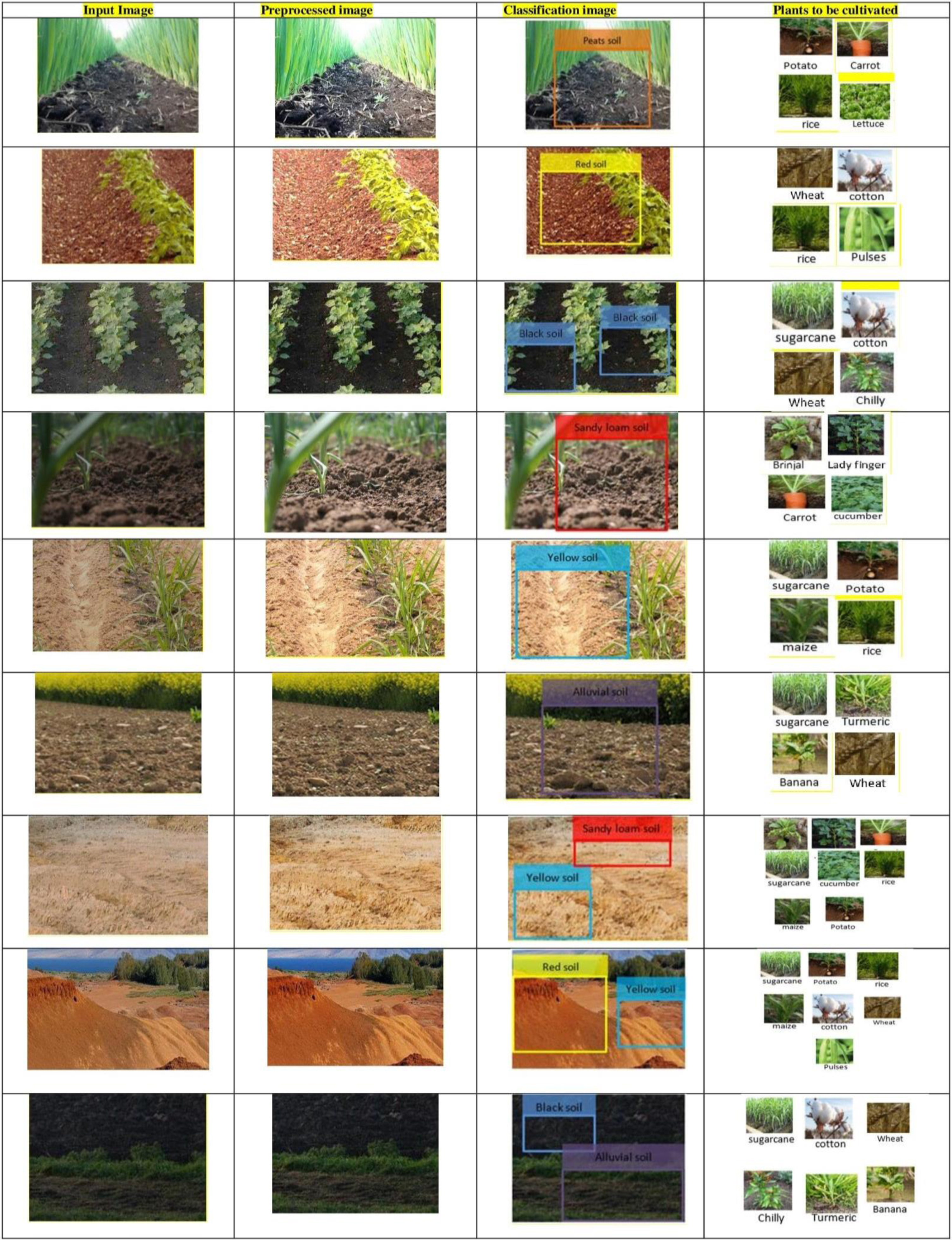
Classification Result with crop recommendation.
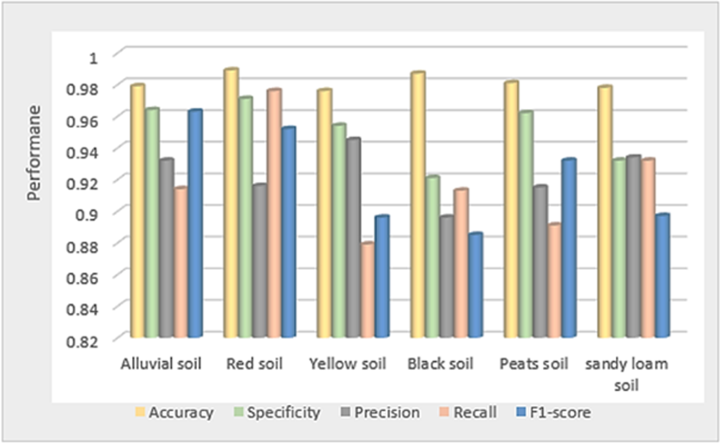
In this study, the performance analysis was calculated via specificity, precision, accuracy, F1 score, and Recall.
Table 2 provides an illustration of different types of soil prediction with specific parameters. The average accuracy, specificity, precision, recall, and F1score of the proposed AQU-FRC Net are 98.16 %, 95.08%, 92.30%, 91.75%, and 92.08% respectively. Whereas Fig. 7 graphically presents the accuracy, specificity, precision, recall, and F1 score.
The ROC was generated for six classes that include black soil, red soil, Alluvial soil, peats soil, sandy loam soil, and yellow soil illustrated in Fig. 8. The proposed AQU-FRC Net achieved higher AUC of 0.987, 0.982, 0.979, 0.975, 0.972, and 0.969 for red soil, black soil, peats soil, Alluvial soil, sandy loam soil, and yellow soil respectively can be measured via True Positive Rate and False Positive Rate metrics.
Efficiency of the proposed AQU-FRC Net Framework
Performance metrics of the proposed soil prediction model.
Where FP TP, FN, and TF, specify false-positives, true-positives, false- negatives, and true-negatives, respectively.
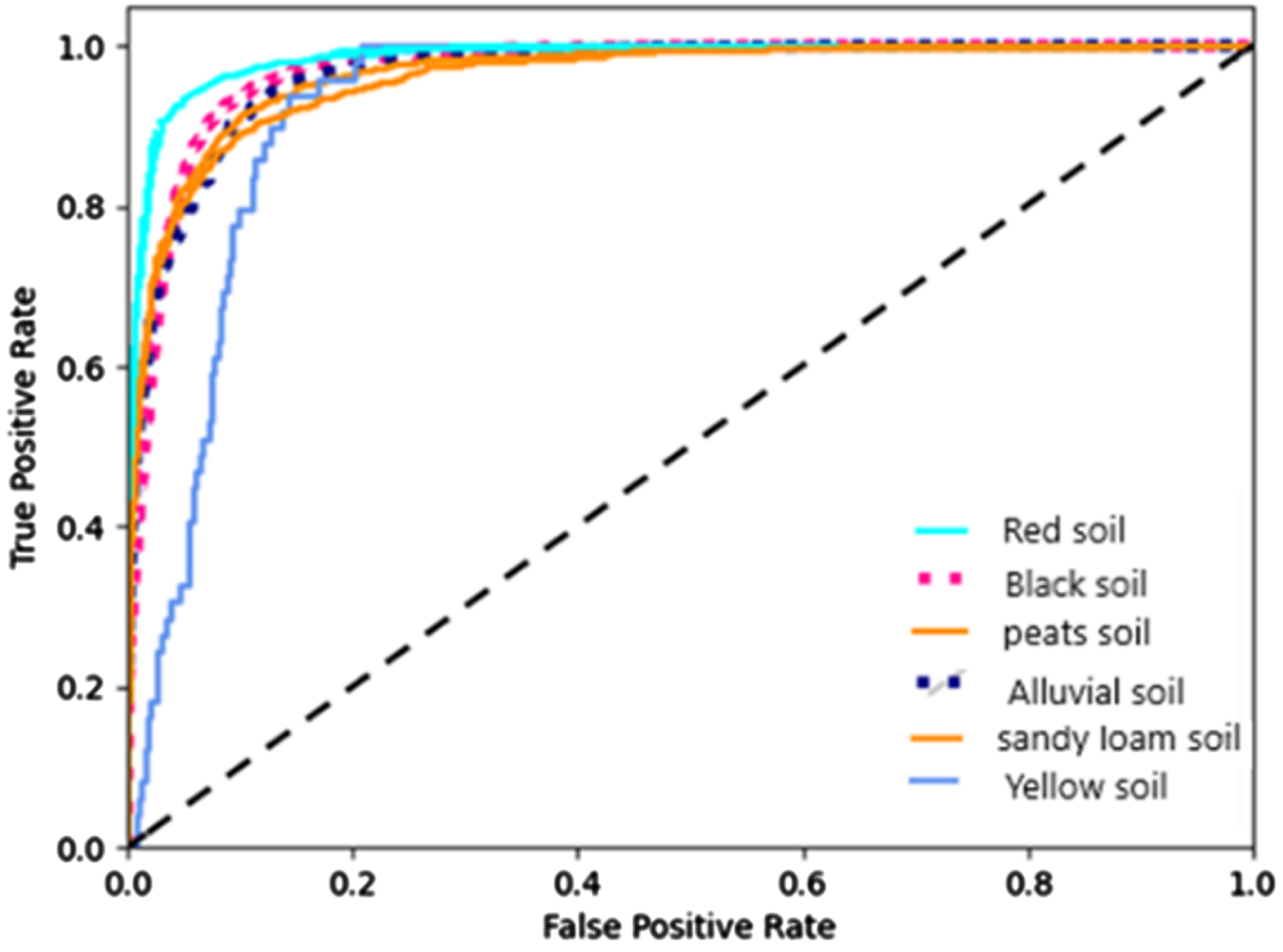
ROC curve of the proposed soil prediction model.
Figure 9 displays the accuracy curve with epochs and accuracy on both axes, the accuracy of the method improves when the epochs are increased. The epoch vs loss graph in Fig. 10 depicts how the loss of the model decreases when the epochs are improved. So, the predicted accuracy of 98. 16 % for the proposed AQU- FRC Net are highly reliable for soilprediction.
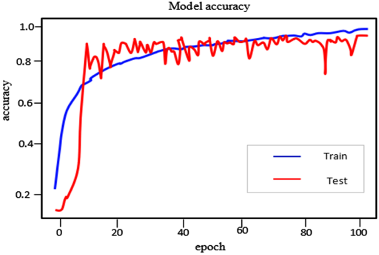
Performance curve of the proposed soil prediction model.
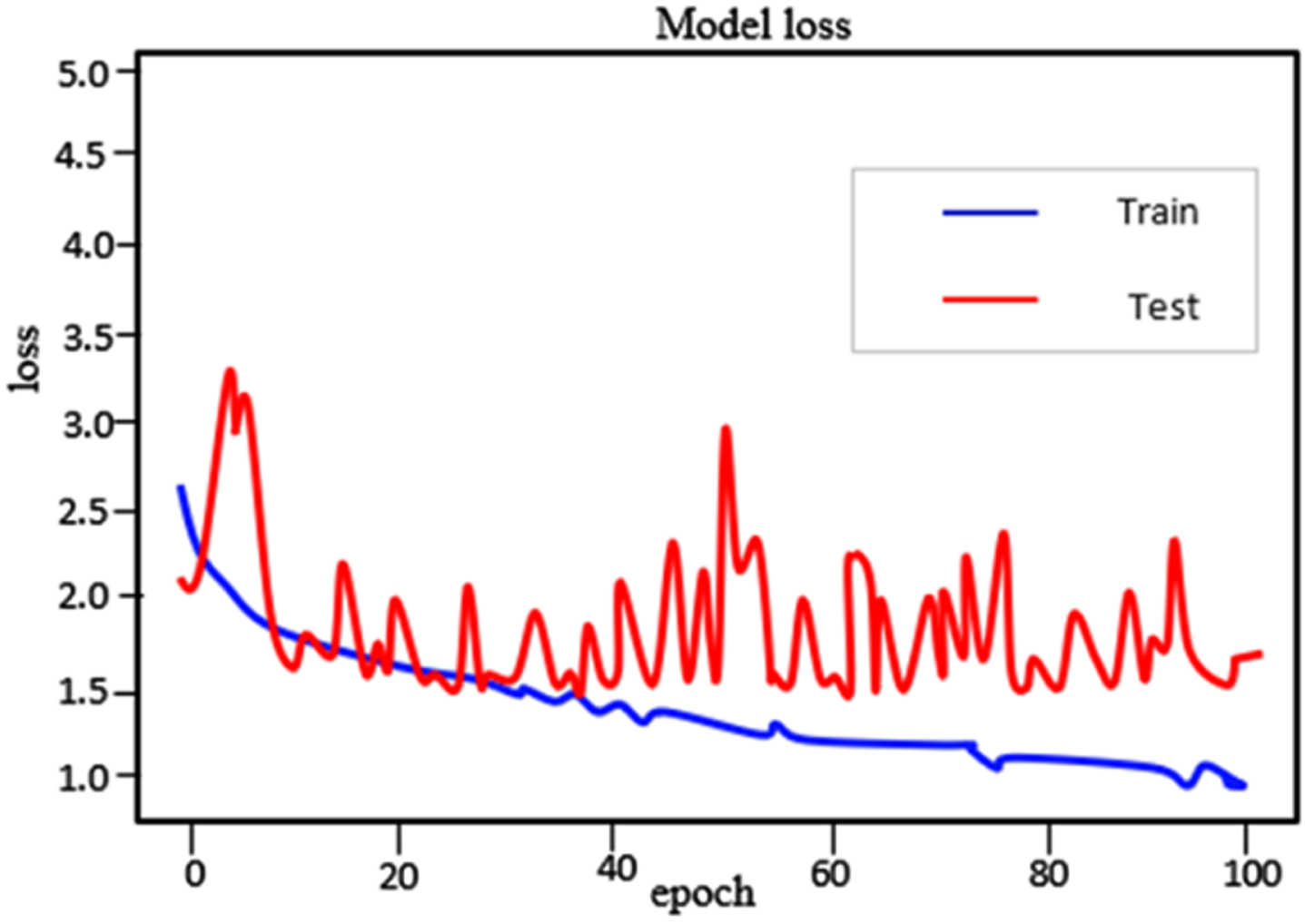
Loss curve of proposed soil prediction model.
Comparison of traditional DL techniques.
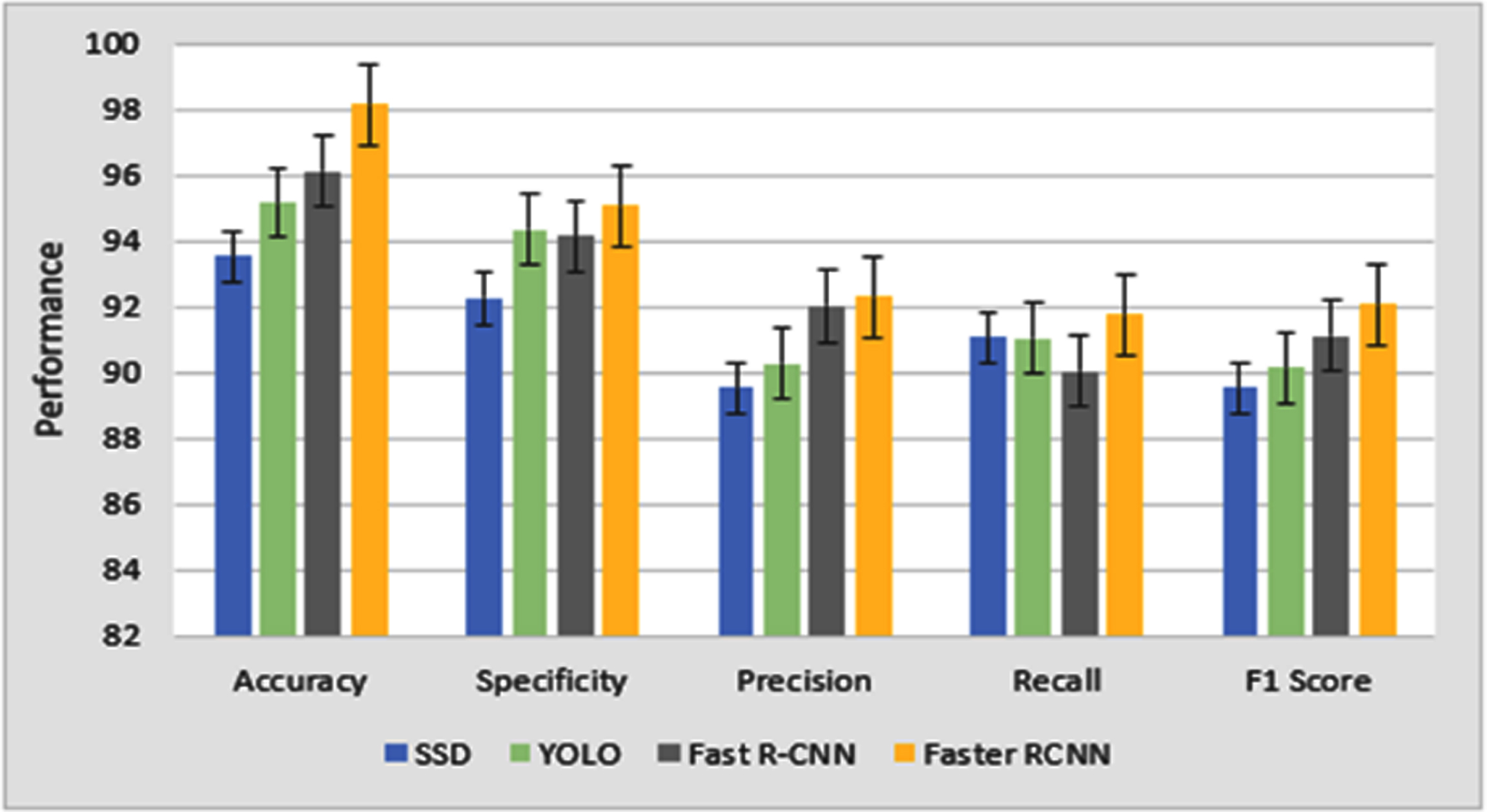
For evaluating the effectiveness of the proposed model, the existing soil prediction methods were compared to the findings of the proposed technique. The efficiency is analyzed based on the accuracy, specificity, precision, Recall, and F1 score metrics. The proposed model’s performance is compared with three conventional approaches such as single-shot detector (SSD), You Only Look Once (YOLO), and Fast R-CNN, corresponding findings are illustrated in Fig. 11
The plot depicts the accuracy obtained by SSD, YOLO, and Fast R-CNN is 93.52%, 95.16%, and 96.13% respectively. Compared to the traditional network, the proposed method achieved 4.64%, 3%, and 2.03% higher performance than SSD, YOLO, and Fast R-CNN respectively. Thus, it is seen that AQU-FRC Net performs better than other existing models.
Table 3 compares the proposed model with other existing methods. The proposed AQU-FRC Net achieves 98.16 % of accuracy, which is better than the existing model.
Comparison between the proposed and the existing models
Comparison between the proposed and the existing models
An ablation study was made to assess the efficiency of the Aquila optimization utilized in the optimization stage. In this experiment, with Aquila optimization and without Aquila optimization as illustrated in Fig. 12. According to a comparison, the performance was estimated in terms of Accuracy, specificity, precision, Recall, and F1 score. According to our findings, the prediction of soil using ablation models was typically less accurate than using Aquila optimization, which proves the usefulness of the Aquila optimization in the prediction process of the proposed AQU- FRC Net.
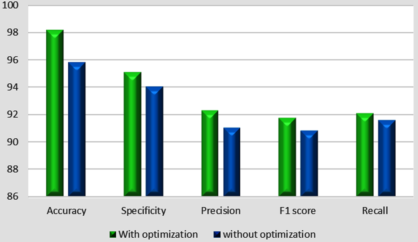
Performance comparison in ablation study with and without optimization.
The effectiveness of the proposed AQU- FRC Net was evaluated and the ablation is performed with and without Aquila optimization. There is a possibility that the model without Aquila optimization had the lowest accuracy. From this analysis, we have concluded that the proposed model with Aquila optimization gives high accuracy in the prediction of soil.
In this paper, a novel approach is proposed for predicting the soil types using AQU-FRC Net and recommending the crops based on soil - the crop relationship database. Initially, the soil images were preprocessed using a scalable range-based adaptive bilateral filter for eliminating the noise artifacts from the images. The pre-processed soil images were classified using Faster R-CNN which utilized MobileNet as a feature extraction network. The classifier model was optimized by the Aquila optimization algorithm that normalizes the parameters of the network to achieve better results. The proposed AQU-FRC Net achieves a high accuracy of 98.16% and a specificity of 95.08% for predicting soil types. From this research, it can be stated that the proposed method is more accurate than the existing method in terms of predicting soil types. In the future, more crops and soil were added and the proposed model will be built and integrated into the smartphone app. The proposed AQU-FRC Net also provides fertilizer recommendations in future.