Some new types of generalized fuzzy real numbers

Abstract

This study provides the generalization of fuzzy real numbers by imposing the elevator’s condition upon it’s legs. Our aim is to construct three types of Lift Fuzzy Real Numbers, an extension of h-generalized fuzzy real numbers, to indicate medical signals, stock market values, and commercial establishment profits over time. It explores concepts like ɛ-cut, strong ɛ-cut, β-level set, and convexity, and presents a graphical representation based on profit earned by three industries. Appropriate numerical examples are provided to support the new ideas. It’s interesting to note that Lift Fuzzy Real Numbers are also used to represent real numbers. Additionally, the connections between the Lift Fuzzy real numbers have been established. The new fuzzy real numbers offer an advantage in representing data sets not represented by existing fuzzy numbers.

MSC 2010:03E72

1 Introduction

Uncertainty and vagueness are inevitable in real life situations. The concept of fuzzy sets was established by Zadeh [1] to examine these circumstances. Following this, Chang and Zadeh [2] initiated the study of fuzzy real numbers in 1972 which was enhanced by Dubois and Parade [3] in 1978. Through the use of a fuzzy number’s fuzzy expectation, Z-number was transformed into a classical fuzzy number by Kang et al. [4], which is fairly significant for further applications. Fernández & Úbeda [5] introduced the concept of quasilineability and researched topological properties of the set of fuzzy numbers. (L,R)-fuzzy numbers, where L is an increasing function and R is a decreasing function of real variables, is the most well-known theory of fuzzy numbers. In perspective of the shapes of L and R, the fuzzy numbers are categorized as triangular fuzzy numbers, trapezoidal fuzzy numbers, pentagonal fuzzy numbers, etc. M. Koppula et al. [6] defined 2n+1 and 2n fuzzy numbers, which is the generalization of triangular and trapezoidal fuzzy numbers. Sudha and Jayalalitha [7] explained a few theoretical components of Fuzzy Triangular Numbers in Sierpinski Triangle. Raj and their Collaborator’s [8] predicted certain kind of arithmetical operations on trapezoidal fuzzy numbers to optimize the transportation cost byapplying it. Thiruppathi and Kirubhashankar [9] solved assignment problem using hexagonal fuzzy numbers in the fuzzy environment.

The interval valued fuzzy number was invented by Wang and Li [10], as the usual fuzzy numbers cannot accurately describe the vagueness. Lee et al. [11] studied new fuzzy multiple criteria decision making model based on interval-valued fuzzy numbers to tackle the supplier selection problem in the circumstances where uncertainty is introduced. Bisht & Dangwal [12] resolved the interval valued transportation problem by translating it to octagonal fuzzy transportation problem.

Burillo [13, 14] presented a definition of intuitionistic fuzzy numbers in 1994 and studied perturbations of intuitionistic fuzzy number and the first properties of the correlation between these numbers. In order to choose the optimal location for a manufacturing plant, Rasheed et al. [15] suggested an intuitionistic fuzzy aggregative investment benefit rate in which respondents indicated both linguistic variable membership function and non-membership function with some hesitancy level. Xu [16] outlined the concept of the score function and accuracy function of interval valued intuitionistic fuzzy number. Pathinathan, & Minj [17] introduced interval valued pentagonal fuzzy numbers.

Various kinds of fuzzy real numbers were examined, and their applicability in numerous fields were studied. Generalized fuzzy number was introduced by Chen and Hsieh [18], which persuades more recognition in solving many real life problems. Adabitabar Firozja [20] and their collaborators proposed ranking by contrasting fuzzy real numbers with generalized fuzzy numbers. Chi and Yu [19] examined ranking of generalized fuzzy numbers with different heights. To improve upon the existing ranking techniques, Sam’an and Dasril [21] researched ranking in the ideas of left and right interval type-2 generalized trapezoidal fuzzy numbers. In the area of fuzzy risk analysis, Chen and Chen [22], Patra et al. [23, 24], researched generalized trapezoidal fuzzy real numbers. Hsieh [25] discussed similarity measure of generalized fuzzy numbers and Sen et al. [26] discussed that of generalized trapezoidal fuzzy numbers. Kaur and Kumar [27] solved fuzzy transportation problems using generalized trapezoidal fuzzy numbers. The existing theory of generalized fuzzy real number defined by Chen and Hsieh [18] fails to meet some requirements, a new generalization of fuzzy numbers was improved by Zhang, Guo, Chen [28] and this generalized fuzzy number is called h –generalized fuzzy real number where 0 < h≤1 and h is the height of the fuzzy number. Patra and Mondal [29] introduced a new similarity measure using geometric distance, area and height of two generalized trapezoidal valued fuzzy numbers which is possible to calculate the similarities when the height of any one of two generalized trapezoidal fuzzy numbers becomes zero. A set of data whose minimum value is zero for a predetermined maximum value will be analyzed by the existing fuzzy numbers. However, certain sets of data contain minimum values that are genuinely strictly greater than zero. For instance, the majority of real-world data sets— such as those pertaining to health, market value, profit, etc. — have non-zero minimum values. The signals that reflect the aforementioned data sets cannot be represented by existing fuzzy real numbers. Furthermore, the real axis may not be met by these signals. Signals like square waves, sine waves, cosine waves, triangle waves, etc. that are employed in engineering and scientific signal processing procedures will be represented by fuzzy numbers. Such signals will require fuzzy arithmetic operations for processing. The identical spacing between the loops of the aforementioned waves makes this possible. But the majority of medical signals lack this quality. As a loop of a fuzzy number starts from a point in the real axis and ends at a point in the real axis, existing types of fuzzy numbers are not suitable to analyze such data sets. In order to represent such data sets in the fuzzy environment, new types of fuzzy sets on the real line are introduced namely, Left Lift Fuzzy Real Number (LLFRN), Right Lift Fuzzy Real Number (RLFRN), and Lift Fuzzy Real Number (LFRN). Furthermore the basic properties of the proposed generalizations of fuzzy numbers are investigated.

This paper consists of seven sections. Following the introduction, second section deals with certain basic concepts and results, taken from Zadeh [1], Klir and Yuvan [30] and Zhang et al. [28]. The third section deals with analysis of fuzzy numbers using graphs, which gives a motivation to introduce three types of fuzzy real numbers. New types of fuzzy real numbers are introduced in the fourth section and their applications to the data sets on profits made by industries are analyzed in the fifth section. The advantages and disadvantages of the proposed fuzzy real numbers are described in Section six. Section seven concludes this paper

Throughout this paper $ℝ$ denotes the set of all real numbers and F( $ℝ$ ) denotes the collection of all fuzzy sets of $ℝ$ . In this paper, the letters a, b, c, d always denote the real numbers with a≤c ≤ d≤b and 0 < β≤1.

2 Preliminaries

Let X be a space of points. The members of X are denoted by x. A fuzzy set [1, page 339] A in X is characterized by a membership function f _A (x) which associates with each point in X a real number in the interval [0, 1], with the value of f _A (x) at x representing the grade of membership of x in A. The fuzzy set A in X can also be represented as A = {(x, f _A (x)): x∈X} where f _A : X⟶[0, 1] is a function from X to [0, 1], known as a membership function of the fuzzy set A in X. For any α∈[0, 1], the α-cut ^αA and the strong α-cut ^α +A [30, page 19] are defined as the crisp sets ^αA = {x: f _A (x)≥α} and ^α +A = {x: f _A (x) > α} respectively. The support [30, page 21] of a fuzzy set A within the universal set X is the crisp set that contains all the elements of X that have nonzero membership grades in A. Evidently the support of A is the same as the strong α-cut of A for α= 0, denoted by ^0 + A or supp(A). The 1-cut, ¹A = {x: f _A (x)≥1} = {x: f _A (x) = 1} = f _A ^–1({1}) is called the core [30, page 21] of A. The height, h(A) [30, page 21], of a fuzzy set A is the largest membership grade obtained by any element in that set. That is h(A) = sup {f _A (x): x∈X}. A fuzzy set A is normal [30, page 21] when h(A) = 1; it is called subnormal when h(A) < 1. The height of A may also be viewed as the supremum of α for which ^αA≠ Ø. A fuzzy set A is convex [1, page 347] if the α-cuts ^αA = {x: f _A (x)≥α} are convex for all α∈(0,1]. Equivalently, A is convex if and only if f _A (λx+(1-λ)y)≥min{f _A (x), f _A (y)}.

Definition 2.1. (cf. [30, page 97])

A fuzzy set A of $ℝ$ is a fuzzy real number if it possesses the following three properties:

A must be a normal fuzzy set;

^αA must be a closed interval for every α∈(0, 1];

the support of A, ⁰⁺ A, must be bounded.

$\mathfrak{F}$ ( $ℝ$ ) denotes the collection of all fuzzy real numbers where fuzzy real numbers are fuzzy numbers in the sense of Klir and Yuan [30].

The next lemma gives the structure of a fuzzy real number.

Lemma 2.2. [30, Theorem 4.1, page 98]

Let A $\in \mathfrak{F}$ ( $ℝ$ ). Then, A is a fuzzy real number if and only if there exists a closed interval [a, b] ≠ Ø such that $f_A\left(x\right)=\{\begin{array}{c}1\mathit{for}x\in \left[a,b\right]\\ L\left(x\right)\mathit{for}x\in \left(-\infty ,a\right)\\ R\left(x\right)\mathit{for}x\in \left(b,\infty \right)\\ \end{array}$(1) where L is a function from (−∞, a) to [0, 1] that is monotonic increasing, continuous from the right, and such that L(x) = 0 for every x ∈ (− ∞ , ω₁), ω₁≤a; R is a function from (b, ∞) to [0, 1] that is monotonic decreasing, continuous from the left, and such that R(x) = 0 for every x∈ (ω₂, ∞), ω₂≥b.

Remark 2.3.

Since fuzzy real numbers are characterized by the functions L and R,they are also called L-R fuzzy real numbers.

Definition 2.4. [28, Definition 3.1, page 65]

Let 0 < h≤1 and let A be a fuzzy set in $ℝ$ . Then A is said to be a h-generalized fuzzy real number if it satisfies the following conditions:

A is h-normal that is there exists x₀ $\in ℝ$ , such that f _A (x₀) = h = the height of A.

f _A : $ℝ⟶$ [0, h] is upper semi-continuous,

A is fuzzy convex,

The support of A is bounded.

3 Materials and methods

It is evident from Lemma 2.2, that every fuzzy number can be represented in the form of (1) whose graph is illustrated in [30, Fig. 4.3, page 100]. As a result, the graph of a fuzzy real number gradually climbs from a point on the real axis to its highest point and then gradually declines from there to a point on the real axis. Real-world problems occasionally have data that cannot be captured by graphs of fuzzy real values. For instance, we take into account information about a company’s market worth and information about a diabetic patient’s blood sugar levels during a certain time frame. A company’s market value on the stock exchange may rise from a fixed positive value to a maximum value or fall from the maximum value to a positive or non-negative value. The statement that a market value never falls to zero is always true. In the medical field, a diabetic patient’s blood sugar level may rise from the lower limit of the normal blood sugar range to an abnormal level and, following therapy over time, may fall from the abnormal level to a level in the normal blood sugar range. Similar case is also applicable to blood pressure of a patient. As previously mentioned, the current concept of fuzzy real numbers is insufficient to simulate the aforementioned circumstances. In order to describe the data connected to the aforementioned conditions and predict future values of the parameter (stock prices, sugar levels, and pressure value etc.), fresh versions of fuzzy real numbers are introduced in this research.

3.1 Graph analysis of a fuzzy real number

Let A be an L -R fuzzy real number with support [a, b] and core [c, d]. It is interesting to observe that graph {(x, f _A (x)): a≤x≤b} of its membership function f _A with domain [a, b] is bounded by the lines y = 0 and y = 1 that are known as lower-level and upper-level of f _A . The points (a, 0), (b, 0) are called the lower-level points and (c, 1), (d, 1) are the upper-level points of f _A . The vertical lines x = c, x = d may be called the splitting lines of f _A . Therefore (a, 0) lying in the left of x = c is called the lower-level point of L and (b, 0) lying in the right of x = d is called the lower-level point of R. The point (c, 1) is called the upper-level point of L and (d, 1) is that of R. The level points (a, 0), (b, 0) and (c,1), (d,1) play a vital role in defining new types of generalized fuzzy real numbers. Chen, Hsieh [18] and Zhang, Guo, Chen [28] studied generalized fuzzy real numbers by replacing the upper-level points (c, 1), (d, 1) by (c, h), (d, h) respectively. The following three types of fuzzy sets in $ℝ$ will be used to introduce three versions of fuzzy numbers.

Case-(i):The upper-level point (c, 1) may be replaced by (c,β) and left lower-level point (a, 0) may be replaced by (a, α) where 0≤α≤β≤1. This case leads to define an Left Lift Fuzzy Real Number with height β and lifted left at α.

Case-(ii): The upper-level point (d,1) may be replaced by (d,β) and right lower-level point (b, 0) may be replaced by (b, γ) where 0≤γ≤β≤1. This case leads to define a Right Lift Fuzzy Real Number with height β and lifted right at γ.

Case-(iii):The upper-level points (c, 1), (d, 1) may be respectively replaced by (c, β), (d, β) and lower-level points (a, 0), (b, 0) may be respectively replaced by (a, α), (b, γ) where 0≤α≤β≤1 and 0≤γ≤β≤1. This case leads to define a Lift Fuzzy Real Number with height β and lifted left at α, lifted right at γ.

4 Results and discussion

In this section some new types of fuzzy real numbers are introduced with examples and their basic properties are discussed.

Let A be a fuzzy set in $ℝ$ and α, β, γ∈ [0, 1] with 0≤α≤β≤1, 0≤γ≤β≤1.

Definition 4.1

Let 0≤α≤β≤1 and let A be a fuzzy set in $ℝ$ with support lying in [a, b]. Then A is said to be a Left Lift Fuzzy real number (briefly LLFRN) with height β andleft lift at α if there is an interval [c, d] ⊆ [a, b] and the membership function f _A of A which is defined as $f_A\left(x\right)=\{\begin{array}{c}\beta \mathit{for}x\in \left[c,d\right]\\ L\left(x\right)\mathit{for}x\in \left(-\infty ,c\right)\\ R\left(x\right)\mathit{for}x\in \left(d,\infty \right)\\ \end{array}$(2) where L is an increasing function from (−∞, c] to [0, 1], continuous from the right with L(x) = 0 for −∞< x < a, L(a) =α and R is a decreasing function from [d, ∞) to [0, 1], continuous from the left with R(x) = 0 for b < x < ∞.

Depending upon the parameters α,β, “left lift” = ”ll” real numbers a,b,c,d and the functions L _A , R _A ,we use the notation A ^ll to represent the LLFRN A.

Symbolically, A ^ll  = [f _A : a≤c≤d≤b; L _A , R _A ;(α, β, –)],where ‘–‘ indicates that there is no restriction for the right lift that is the right lift may be zero or greater than zero.

If L _A and R _A are linear on [a, c] and [d, b] respectively then we write A ^ll  = [f _A : a≤c≤d≤b; (α, β, –)] which is known as a linear type LLFRN or briefly LLLFRN.

The following abbreviations will be used in sequel.

LLF( $ℝ$ ) = {A ^ll : a, b, c, d∈ $ℝ$ ; 0≤α≤β≤1}.

LLF( $ℝ$ )([a, b]) = {A ^ll : c, d∈ [a, b]; 0≤α≤β≤1}.

LLF( $ℝ$ )(a≤c≤d≤b) = {A ^ll : 0≤α≤β≤1}.

Remark 4.1.1.

LLF( $ℝ$ )(a≤c≤d≤b) ⊆LLF( $ℝ$ )([a, b])⊆LLF( $ℝ$ ).

The next remark follows easily from (2).

Remark 4.1.2.

If A ^ll ∈LLF( $ℝ$ )(a≤c≤d≤b) then f _A ^–1(β) = [c, d].

Proposition 4.1.3.

Every real number x can be represented by the family of LLFRNs.

Proof.

Let x be a real number. For every β∈ (0, 1], let A be a fuzzy set in $ℝ$ with height β and support = {x} whose membership function is defined as $f_A\left(t\right)=\{\begin{array}{c}\beta \mathit{for}t=x\\ 0\mathit{otherwise}\\ \end{array}$ which satisfies the requirements for a LLFRN with height β and left lift at 0. Thus every member of the family { ${\left(A\right)}_{\beta }^{\mathit{ll}}$ : β∈(0, 1], height of A =β, support of A = x} represents the real number x.

Here a = b = c = d = x. This completes the proof.

Theorem 4.1.4.

LetA ^ll ∈LLF( $ℝ$ ) with height β.

The ɛ- cut of A is a closed interval for every ɛ with 0 < ɛ≤β.

The strong ɛ-cut of A is an interval for every ɛ with 0 < ɛ< β.

The β-level set {x:f _A (x) =β} of A is f _A ^–1(β) = [c, d].

Support of A is bounded.

f _A : $ℝ⟶$ [0, β] is upper semi-continuous.

A is fuzzy convex.

Proof. Let A ^ll  = [f _A : a≤c≤d≤b; L _A , R _A ; (α,β,–)].

Let 0 < ɛ≤β.

The proof for the assertion (i) is divided into three cases namely Case (i): ɛ=β, Case (ii): α≤ɛ< β and Case (iii): 0 < ɛ< α.

Case-(i): ɛ=β.

The ɛ-cut of A =  ^ɛA = {x: f _A (x)≥ɛ}

 = {x: f _A (x)≥β}

 = {x: f _A (x) =β} = [c, d].

The strong ɛ-cut of A =  ^ɛ +A = {x: f _A (x) > ɛ}

 = {x: f _A (x) > β} =Ø which is a null interval.

Case-(ii): α≤ɛ< β.

Since f _A is increasing on [a, c], choose x₁such that x₁ = inf {x∈[a, c]:f _A (x) =ɛ}.

Since f _A is continuous on [a, c],f _A (x₁) =ɛ.

The proof for this case can be given in three steps namely Step-1: f _A (b) < ɛ, Step-2: f _A (b) =ɛ and

Step-3: f _A (b) > ɛ.

Step-1: f _A (b) < ɛ.

Since f _A is decreasing on [d, b], choose x₂such that x₂ = sup{ x∈[d, b]:f _A (x) =ɛ}.

Therefore ^ɛA = [x₁, x₂] and ^ɛ +A = (x₁, x₂).

Step-2:f _A (b) =ɛ.

Here x₂ = b. Therefore ^ɛA = [x₁, b] and ^ɛ +A = (x₁, b).

Step-3:f _A (b) > ɛ.

Clearly f _A (x) > ɛ for all x∈[d, b] and hence ^ɛA = [x₁, b] and ^ɛ +A = (x₁, b].

Case-(iii): 0 < ɛ< α.

Clearly f _A (x) > ɛ for all x∈[d, b].

Since f _A is decreasing on [d, b], choose x₂such that x₂ = sup{x∈[d, b]:f _A (x) =ɛ}.

Since f _A is continuous on [d, b], f _A (x₂) =ɛ.

The proof for this case can be given in three steps namely Step-4: f _A (b) < ɛ, Step-5: f _A (b) =ɛ and

Step-6:f _A (b) > ɛ.

Step-4:f _A (b) < ɛ.

By choosing x₂ as in Step-1 of Case-(ii), we have

^ɛA = [a, x₂] and ^ɛ +A = [a, x₂].

Step-5:f _A (b) =ɛ.

Proceeding as in Step-2 of Case-(ii), ^ɛA = [a, b] and

^ɛ +A = [a, b).

Step-6:f _A (b) > ɛ.

Clearly f _A (x) > ɛ for all x∈[d, b] and hence ^ɛA = [a, b] =  ^ɛ +A.

This proves (i), (ii) and (iii).

The support of A = ^0 + A = {x: f _A (x) > 0} ⊆ [a, b] that implies the support of A is bounded which proves (iv).

f _A : $ℝ⟶$ [0, β] is upper semi-continuous ⇔ for every ɛ∈[0, β], the set f _A ^–1((ɛ, β]) is an open set in the real line.

Now ɛ∈ [0, β]

⇒ there are x₁, x₂ with x₁≤x₂ and f _A (x₁) = f _A (x₂) =ɛ.

⇒ f _A ^–1((ɛ, β]) = {x: f _A (x)∈(ɛ, β]}

 = {x: ɛ< f _A (x)≤β}

 = {x: β≥f _A (x) > ɛ} = (x₁, x₂).

Thus we get an open interval in the real line which is an open set in the real line. This proves (v).

Now to prove (vi) let ɛ∈ [0, β] and x, y∈ $ℝ$ with a≤x≤y≤b.

Then ɛx+(1-ɛ)y≤ɛy+(1-ɛ)y = y and

ɛx+(1-ɛ)y≥ɛx+(1-ɛ)x = x

⇒ɛx+(1-ɛ)y∈ [x, y] so that x≤ɛx+(1-ɛ)y≤y.

Let z =ɛx+(1-ɛ)y and therefore z∈ [x, y] so that

x≤z≤y.

In order to establish (vi), six cases for x, y have to be considered.

Suppose a≤x≤c. This leads to three cases.

Case-(i):

a≤x≤y≤c.

As L is increasing on [a, c], L(x)≤L(z)≤L(y) which implies min{f _A (x), f _A (y)} = f _A (x) = L(x) so that

f _A (z)≥f _A (x) = min{f _A (x), f _A (y)}.

Case-(ii):

a≤x≤c≤y≤d.

Since f _A (y) = 1, min{f _A (x), f _A (y)} = f _A (x).

If z≤c then f _A (z)≥f _A (x) = min{f _A (x), f _A (y)}.

If c≤z then f _A (z) = 1≥f _A (x) = min{f _A (x), f _A (y)}.

Case-(iii):

a≤x≤c≤d≤y≤b.

Suppose min{f _A (x), f _A (y)} = f _A (x). Then f _A (x)≤f _A (y).

If z∈ [a, c], then f _A (x)≤f _A (z).

If z∈ [c, d], then f _A (x)≤1 = f _A (z).

If z∈[d, b], then z∈ [d, y] so that f _A (x)≤f _A (y) ≤f _A (z).

Therefore

f _A (z)≥min{f _A (x), f _A (y)} when min{f _A (x), f _A (y)} = f _A (x).

The case when min {f _A (x), f _A (y)} = f _A (y), can be similarly discussed.

Now suppose c≤x≤d. Thisleads to two cases.

Case-(iv):

c≤x≤y≤d.

Since z∈[x, y], f _A (x) = f _A (y) = f _A (z) = 1 that implies f _A (z)≥min{f _A (x), f _A (y)}.

Case-(v):

c≤x≤d≤y≤b.

f _A (x) = 1≥f _A (y) so that min {f _A (x), f _A (y)} = f _A (y).

If z∈ [c, d] then f _A (z) = 1≥f _A (y) = min{f _A (x), f _A (y)}.

If z∈ [d, b] then z∈ [d, y] so that d≤z≤y that implies f _A (z)≥f _A (y) = min{f _A (x), f _A (y)}.

Now suppose d≤x≤b.

This leads to only one case.

Case-(vi):

c≤d≤x≤y≤b.

Clearly d≤x≤z≤y≤b so that f _A (z)≥f _A (y) ≥f _A (x) that implies f _A (z)≥f _A (y) = min{f _A (x), f _A (y)}.

From the above six cases it follows that f _A (ɛx+(1-ɛ)y)≥min{f _A (x), f _A (y)} that implies Ais fuzzy convex. This proves (vi) and proof of the theorem is completed.

Corollary 4.1.5. A ^ll  = [f _A : a≤c≤d≤b; L _A , R _A ; (α,β,–)] is a β-generalized fuzzy number.

Proof.

The proof follows from Theorem 4.1.4. and Definition 2.4.

Example 4.1.6.

Define $f_A\left(x\right)=\{\begin{array}{c}\beta \mathit{for}x\in \left[c,d\right]\\ \alpha +\left(\beta -\alpha \right)\left(\frac{x-a}{c-a}\right)\mathit{for}a⩽x⩽c\\ \beta \left(\frac{b-x}{b-d}\right)\mathit{for}d⩽x⩽b\\ 0\mathit{otherwise}\\ \end{array}$(3) where c ¬= a, b ¬= d, $L\left(x\right)=\{\begin{array}{ccc}0& \mathit{for}& x<a\\ \alpha +\left(\beta -\alpha \right)\left(\frac{x-a}{c-a}\right)& \mathit{for}& a⩽x⩽c\\ \end{array}$

and $R\left(x\right)=\{\begin{array}{ccc}\beta \left(\frac{b-x}{b-d}\right)& \mathit{for}& d⩽x⩽b\\ 0& \mathit{for}& x>b\\ \end{array}$

Then A ^ll  = [f _A : a≤c≤d≤b; L _A , R _A ; (α,β,–)] so that A with membership function f _A in (3), is a LLFRN with height β and left lift at α.

By taking a = 2,b = 8, c = 4, d = 6, α= 0.4 and β= 0.7 in (3) we have $f_A\left(x\right)=\{\begin{array}{ccc}0.7& \mathit{for}& x\in \left[4,6\right]\\ \frac{\left(0.2\right)+\left(0.3\right)x}{2}& \mathit{for}& 2⩽x⩽4\\ \left(0.7\right)\left(\frac{8-x}{2}\right)& \mathit{for}& 6⩽x⩽8\\ 0& & \mathit{otherwise}\\ \end{array}$(4)

where $L\left(x\right)=\{\begin{array}{ccc}0& \mathit{for}& x<2\\ \frac{\left(0.2\right)+\left(0.3\right)x}{2}& \mathit{for}& 2⩽x⩽4\\ \end{array}$

and $R\left(x\right)=\{\begin{array}{ccc}\left(0.7\right)\left(\frac{8-x}{2}\right)& \mathit{for}& 6⩽x⩽8\\ 0& \mathit{for}& x>8\\ \end{array}$

Therefore A ^ll  = [f _A :2≤4≤6≤8;L _A , R _A ;(0.4,0.7,–)] so that A with membership function f _A in (4), is a LLFRN with height 0.7 and left lift at 0.4.

Definition 4.2.

Let 0≤γ≤β≤1 and let B be a fuzzy set in $ℝ$ with support lying in [a, b]. Then B is said to be a Right Lift Fuzzy Real Number (briefly RLFRN) with height β and right lift at γ if there is an interval [c, d] ⊆ [a, b] and the membership function f _B of B is defined as $f_B\left(x\right)=\{\begin{array}{ccc}\beta & \mathit{for}& x\in \left[c,d\right]\\ L\left(x\right)& \mathit{for}& x\in \left(-\infty ,c\right)\\ R\left(x\right)& \mathit{for}& x\in \left(d,\infty \right)\\ \end{array}$(5) where L is an increasing function from (−∞, c] to [0, 1], continuous from the right with L(x) = 0 for −∞< x < a and R is a decreasing function from [d, ∞) to [0, 1], continuous from the left with R(x) = 0 for b < x < ∞ and R(b) =γ.

Depending upon the parametersγ,β,“right lift” = ”rl” real numbers a,b,c,d and the functions L _B , R _B , we use the notation B ^rl to represent the RLFRN B.

Symbolically, B ^rl  = [f _B :a≤c≤d≤b; L _B , R _B ;(–, β, γ)],where ‘–‘ indicates that there is no restriction for the left lift that is the left lift may be zero or greater than zero.

If L _B andR _B are linear on [a, c] and [d, b] respectively then we write B ^rl  = [f _B :a≤c≤d≤b; (–, β, γ)] which is known as a linear type RLFRN or briefly LRLFRN.

The following abbreviations will be used insequel.

RLF( $ℝ$ ) = {B ^rl : a, b, c, d ∈ $ℝ$ ; 0≤γ≤β≤1}.

RLF( $ℝ$ )([a, b]) = {B ^rl : c, d ∈ [a, b]; 0≤γ≤ β≤1}.

RLF( $ℝ$ ) (a≤c≤d≤b) = {B ^rl : 0≤γ≤β≤1}.

Remark 4.2.1.

RLF( $ℝ$ )(a≤c≤d≤b)⊆RLF( $ℝ$ )([a, b])⊆RLF( $ℝ$ ).

The next remark follows easily from (5).

Remark 4.2.2.

If B ^rl ∈ RLF( $ℝ$ )(a≤c≤d≤b) then f _B ^–1(β) = [c, d].

Proposition 4.2.3.

Every real number x can be represented by the family of RLFRN.

Proof.

The proof is similar to Proposition 4.1.3.

Theorem 4.2.4.

Let B ^rl ∈RLF( $ℝ$ ) with height β.

The ɛ- cut of Bis a closed interval for every ɛ with 0 < ɛ≤β.

The strong ɛ-cut of B is an interval for every ɛ with 0 < ɛ< β.

The β-level set {x:f _B (x) =β} of B is f _B ^–1(β) = [c, d].

Support of B is bounded.

f _B : $ℝ⟶$ [0, β] is upper semi-continuous.

B is fuzzy convex.

Proof.

The proof is similar to Theorem 4.1.4.

Corollary 4.2.5.

B ^rl  = [f _B : a≤c≤d≤b; (–, β, γ)] is a β-generalized fuzzy number.

Proof.

Follows from Theorem 4.2.4. and Definition 2.4.

Example 4.2.6.

Define $f_B\left(x\right)=\{\begin{array}{cccc}& \beta & \mathit{for}& x\in \left[c,d\right]\\ & \beta \left(\frac{x-a}{c-a}\right)& \mathit{for}& a⩽x⩽c\\ & \gamma +\left(\beta -\gamma \right)\left(\frac{b-x}{b-d}\right)& \mathit{for}& d⩽x⩽b\\ 0& & & \mathit{otherwise}\\ \end{array}$(6) where c ¬= a, b ¬= d $L\left(x\right)=\{\begin{array}{cccc}0& & \mathit{for}& x<a\\ & \beta \left(\frac{x-a}{c-a}\right)& \mathit{for}& a⩽x⩽c\\ \end{array}$

and $R\left(x\right)=\{\begin{array}{ccc}\gamma +\left(\beta -\gamma \right)\left(\frac{b-x}{b-d}\right)& \mathit{for}& d⩽x⩽b\\ 0& \mathit{for}& x>b\\ \end{array}$

Then B ^rl  = [f _B : a≤c≤d≤b; (–, β, γ)] so that B with membership function f _B in (6), is a RLFRN with height β and right lift γ.

By takinga = 2, b = 11, c = 5, d = 8, γ= 0.3 and β= 0.6 in (6) we have $f_B\left(x\right)=\{\begin{array}{ccc}0.6& \mathit{for}& x\in \left[5,8\right]\\ 0.2\left(x-2\right)& \mathit{for}& 2⩽x⩽5\\ \left(1.4\right)-\left(0.1\right)x& \mathit{for}& 8⩽x⩽11\\ 0& & \mathit{otherwise}\\ \end{array}$(7)

where $L\left(x\right)=\{\begin{array}{ccc}0& \mathit{for}& x<2\\ 0.2\left(x-2\right)& \mathit{for}& 2⩽x⩽5\\ \end{array}$

and $R\left(x\right)=\{\begin{array}{ccc}\left(1.4\right)-\left(0.1\right)x& \mathit{for}& 8⩽x⩽11\\ 0& \mathit{for}& x>11\\ \end{array}$

Therefore B ^rl  = [f _B :2≤5≤8≤11; L _B , R _B ; (–, 0.6, 0.3)] so that B with membership function f _B in (7), is a RLFRN with height 0.6 and right lift at 0.3.

Definition 4.3.

Let 0≤α≤β≤1, 0≤γ≤β≤1 and let C be a fuzzy set in $ℝ$ with support lying in [a, b]. Then C is said to be a Lift Fuzzy Real Number (briefly LFRN) with height β and lifts α, γ if there is an interval [c, d] ⊆ [a, b] and the membership function f _C of C is defined as $f_C\left(x\right)=\{\begin{array}{ccc}\beta & \mathit{for}& x\in \left[c,d\right]\\ L\left(x\right)& \mathit{for}& x\in \left(-\infty ,c\right)\\ R\left(x\right)& \mathit{for}& x\in \left(d,\infty \right)\\ \end{array}$(8)

where L is an increasing function from (−∞, c] to [0, 1], continuous from the right with L(x) = 0 for −∞< x < a, L(a) =α and R is a decreasing function from [d, ∞) to [0, 1], continuous from the left with R(x) = 0 for b < x < ∞ and R(b) =γ.

Depending upon the parameters, α, γ, β, “lift” = ”l”,real numbers a,b,c,d and the functions L _C , R _C , we use the notation C ^l to represent the LFRN C.

Symbolically, C ^l  = [f _C :a≤c≤d≤b; L _C , R _C ; (α, β, γ)].

If L _C and R _C are linear on [a, c] and [d, b] respectively then we write C ^l  = [f _C : a≤c≤d≤b; (α, β, γ)] which is known as a linear type LFRN or briefly LLFRN.

The following abbreviations will be used in sequel.

LF( $ℝ$ ) = {C ^l : a, b, c, d∈ $ℝ$ ; 0≤α≤β≤1, 0≤γ≤β≤1}.

LF( $ℝ$ )([a, b]) = {C ^l : c,d∈[a, b]; 0≤α≤β≤1, 0≤γ≤β≤1}.

LF( $ℝ$ )(a≤c≤d≤b) = {C ^l :0≤α≤β≤1,0≤γ≤ β≤1}.

Remark 4.3.1.

LF( $ℝ$ )(a≤c≤d≤b) ⊆LF( $ℝ$ )([a, b])⊆LF( $ℝ$ ).

The next remark follows easily from (8).

Remark 4.3.2.

If C ^l ∈LF( $ℝ$ )(a≤c≤d≤b) then f _C ^–1(β) = [c, d].

Proposition 4.3.3.

Every real number x can be represented by the family of LFRNs.

Proof. The proof is similar to Proposition 3.1.3.

Theorem 4.3.4.

Let C ^l ∈LF( $ℝ$ ) with height β.

The ɛ- cut of C is a closed interval for every ɛ with 0 < ɛ≤β.

The strong ɛ-cut of C is an interval for every ɛ with 0 < ɛ< β.

The β-level set {x:f _C (x) =β} of C is f _C ^–1(β) = [c, d].

Support of C is bounded.

f _C : $ℝ⟶$ [0, β] is upper semi-continuous.

C is fuzzy convex.

Proof.

The proof is similar to Theorem 4.1.4.

Corollary 4.3.5. C ^l  = [f _C :a≤c≤d≤b; L _C , R _C ; (α, β, γ)] is a β-generalized fuzzy number.

Proof.

The proof follows from Theorem 4.3.4. and Definition 2.4.

Example 4.3.6.

Define $f_C\left(x\right)\{\begin{array}{cccc}& \beta & \mathit{for}& x\in \left[c,d\right]\\ & \gamma +\left(\beta -\gamma \right)\left(\frac{x-a}{c-a}\right)& \mathit{for}& a⩽x⩽c\\ & \gamma +\left(\beta -\gamma \right)\left(\frac{b-x}{b-d}\right)& \mathit{for}& d⩽x⩽b\\ 0& & & \mathit{otherwise}\\ \end{array}$(9) where c ¬= a, b ≠  d, $L\left(x\right)=\{\begin{array}{cccc}0& & \mathit{for}& x<a\\ & \gamma +\left(\beta -\gamma \right)\left(\frac{x-a}{c-a}\right)& \mathit{for}& a⩽x⩽c\\ \end{array}$

and $R\left(x\right)=\{\begin{array}{cccc}\gamma +\left(\beta -\gamma \right)\left(\frac{b-x}{b-d}\right)& & \mathit{for}& d⩽x⩽b\\ 0& & \mathit{for}& x>b\\ \end{array}$

Then C ^l  = [f _C : a≤c≤d≤b; L _C , R _C ; (α, β, γ)] so that C with membership function f _C in (9), is a LFRN with height β and lifts α, γ.

By taking a = 2, b = 8, c = 4, d = 6, α= 0.2, γ= 0.4 and β= 0.6 in (9) we have $f_C\left(x\right)=\{\begin{array}{ccc}0.6& \mathit{for}& x\in \left[4,6\right]\\ 0.2\left(x-1\right)& \mathit{for}& 2⩽x⩽4\\ \left(1.2\right)-\left(0.1\right)x& \mathit{for}& 6⩽x⩽8\\ 0& & \mathit{otherwise}\\ \end{array}$(10)

where $L\left(x\right)=\{\begin{array}{ccc}0& \mathit{for}& x<2\\ 0.2\left(x-1\right)& \mathit{for}& 2⩽x⩽4\\ \end{array}$

and $R\left(x\right)=\{\begin{array}{ccc}\left(1.2\right)-\left(0.1\right)x& \mathit{for}& 6⩽x⩽8\\ 0& \mathit{for}& x>8\\ \end{array}$

Therefore C ^l  = [f _C :2≤4≤6≤8; L _C , R _C ; (0.2, 0.6, 0.4)] so that C with membership function f _C in (10), is a LFRN with height 0.6 and lifts 0.2, 0.4.

Theorem 4.3.7.

Every LFRN determines both LLFRN and RLFRN.

If A and B are LLLFRN and LRLFRN respectively and if A ^ll  = [f _A ;a≤c≤d≤b;(α,β,–)] and B ^rl  = [f _B ;a≤c≤d≤b; (–,β,γ)] then they determine a LFRN C with C ^l  = [f _C : a≤c≤d≤b; (α,β,γ)].

Proof.

Let C be a LFRN with membership function f _C and C ^l  = [f _C :a≤c≤d≤b; L _C , R _C ; (α,β, γ)].

By Taking A ^ll  = [f _A : a≤c≤d≤b; L _A ,R_A ;(α,β, –)] with f _A  = f _C and B ^rl  = [f _B :a≤c≤d≤b; L _B , R _B ; (–, β, γ)] with f _B  = f _C we see that A and B are LLFRN and RLFRN respectively.

This proves (i).

Now let A and B be LLLFRN and LRLFRN respectively with A ^ll  = [f _A ;a≤c≤d≤b; (α,β, –)] and B ^rl  = [f _B ;a≤c≤d≤b; (–, β, γ)]

Then C is a LFRN with C ^l  = [f _C ;a≤c≤d≤b; (α,β,γ)].

This proves (ii).

5 Applications to real life problems

This section discusses three fictitious issues with the profits made by the three industries A, B, and C for the calendar year 2022 (January to December 2022).

5.1 Industry A

Industry A initially made a fixed profit, which was then gradually increased until it reached its maximum during the interim period, before being reduced to zero profit at the end of the time. This situation may be represented by LLFRN. The variable ‘x’ may be interpreted as the number of weeks even if the profit was calculated at the end of each month. In other words, the profit made at the end of the first month is identical to the profit made at the end of the fourth week, the profit made at the end of the second month is identical to the profit made at the end of the eighth week, and so on. Even if the profit was determined at the conclusion of every month, this will assist the data analyst in locating the profit at the end of the desired week. There would be a goal profit (or expected profit) for every industry. The membership grade of the month that contributes to the profit would be determined by the ratio of the profit made in a given month to the intended profit. The information in the following table helps to clarify this. Let’s say that industry A’s monthly profit aim is 10 lakhs.

Table 1 can be splintered into two types of tables where the contents of the Table 1 for x = 4,8,12 contribute Table 2 (profit increasing type) and the contents of the Table 1 for x = 16, 20, 24 … 52 contribute Table 3 (Profit decreasing type). In order to represent the data by a LLFRN, the Regression formula is used to find the membership grades.

Table 1

Monthly profit for Industry A

No. of weeks x	Profit	Profit ratio y
4	4000000	0.4
8	6000000	0.6
12	9000000	0.9
16	9000000	0.9
20	4000000	0.4
24	3000000	0.3
28	1000000	0.1
32	0	0
36	0	0
40	0	0
44	0	0
48	0	0
52	0	0

Table 2

Increasing pattern of profit for A

x i	y i
4	0.4
8	0.6
12	0.9

Table 3

Decreasing pattern of profit for A

x i	y i
16	0.9
20	0.4
24	0.3
28	0.1

Using Regression formula for Table 4

Table 4

Computations from Table 2

x i	y i	$x_i-\overline{x}$	$y_i-\overline{y}$	${\left(x_i-\overline{x}\right)}^2$	$\left(x_i-\overline{x}\right)\left(y_i-\overline{y}\right)$
4	0.4	–4	–0.2333	16	0.9332
8	0.6	0	–0.0333	0	0
12	0.9	4	0.2667	16	1.0664
∑x i = 24	∑y i = 1.9		$\sum {\left(x_i-\overline{x}\right)}^2$ = 32	$\sum \left(x_i-\overline{x}\right)\left(y_i-\overline{y}\right)$ = 1.9996

$y-\overline{y}=r\frac{{\sigma }_y}{{\sigma }_x}\left(x-\overline{x}\right)$ $\overline{x}=\frac{24}{3}=8,\overline{y}=\frac{1.9}{3}=0.6333$

and $y-0.6333=0.0624\left(x-8\right)$

That is y = 0.0624x + 0.1341 = p (x)

It can be verified that p(x) is increasing in the interval [4, 12].

Again by using Table 5,

Table 5

Computations from Table 3

x i	y i	$x_i-\overline{x}$	$y_i-\overline{y}$	${\left(x_i-\overline{x}\right)}^2$	$\left(x_i-\overline{x}\right)\left(y_i-\overline{y}\right)$
16	0.9	–6	0.475	36	–2.85
20	0.4	–2	–0.025	4	0.05
24	0.3	2	–0.125	4	–0.25
28	0.1	6	–0.325	36	–1.95
∑x i = 88	∑y i = 1.7			$\sum {\left(x_i-\overline{x}\right)}^2$ = 80	$\sum \left(x_i-\overline{x}\right)\left(y_i-\overline{y}\right)$ = –5

$y=-0.0625x+1.8=q\left(x\right)$

It can be verified that q(x) is decreasing in the interval [16, 28].

Define $f_A\left(x\right)=\{\begin{array}{cc}0.9& 12⩽x⩽16\\ p\left(x\right)& 4⩽x⩽12\\ q\left(x\right)& 16⩽x⩽28\\ 0& \mathit{Otherwise}\\ \end{array}$

The graph of A is illustrated in Fig. 1.

Fig. 1

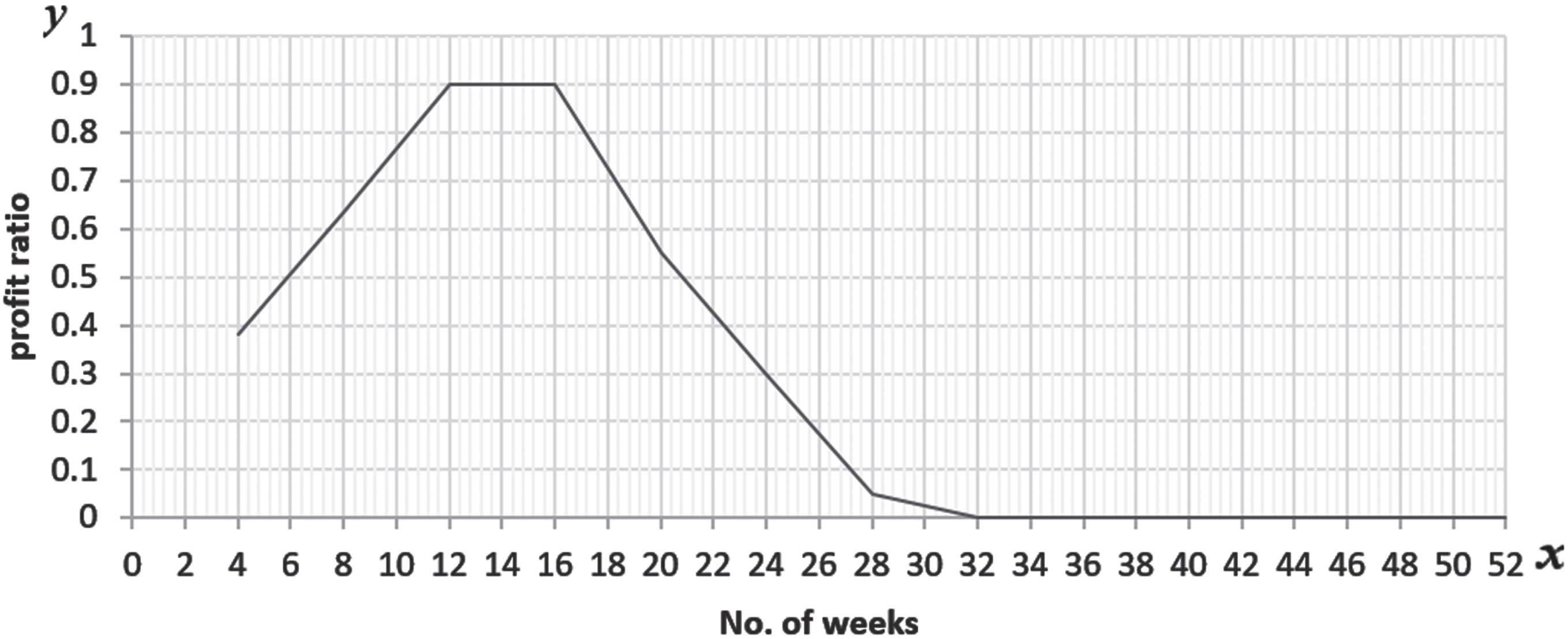
LLFRN.

5.2 Industry B

Industry B initially saw no profit, but that profit eventually climbed to a fixed level and was sustained for a predetermined duration of time. The profit was then reduced to a set sum at the conclusion of the time period. The RLFRN can be used to illustrate this circumstance. Let’s say that 10 lakhs is the monthly target profit for industry B.

Table 6 can be splinted into two types of tables where the contents of the Table 6 for x = 4,8,12,16,20 contribute Table 7 (Profit increasing type) and the contents of the Table 6 for x = 32, 36 … 52 contribute Table 8 (Profit decreasing type). In order to represent the data by a RLFRN use Regression formula to find the membership grades.

Table 6

Monthly profit for Industry B

No. of weeks x	Profit	Profit ratio y
4	0	0
8	2000000	0.2
12	5000000	0.5
16	6000000	0.6
20	8000000	0.8
24	8000000	0.8
28	8000000	0.8
32	8000000	0.8
36	7000000	0.7
40	6000000	0.6
44	5000000	0.5
48	4000000	0.4
52	3000000	0.3

Table 7

Increasing pattern of profit for B

x i	y i
4	0
8	0.2
12	0.5
16	0.6
20	0.8

Table 8

Decreasing pattern of profit for B

x i	y i
32	0.8
36	0.7
40	0.6
44	0.5
48	0.4
52	0.3

Using Table 7 and the method which is discussed in section 5.1, the value of y in the interval [4, 20] is $y=0.05x-0.18=p\left(x\right)$

It can be verified that p(x) is increasing in the interval [4, 20].

Using Table 8 and the method which is discussed in section 5.1, the value of y in the interval [32, 52] is $y=-0.025x+1.6=q\left(x\right)$

It can be verified that q(x) is decreasing in the interval [4, 20].

Define $f_B\left(x\right)=\{\begin{array}{cc}0.8& 20⩽x⩽32\\ p\left(x\right)& 4⩽x⩽20\\ q\left(x\right)& 32⩽x⩽52\\ 0& \mathit{Otherwise}\\ \end{array}$

The graph of B is illustrated in Fig. 2.

Fig. 2

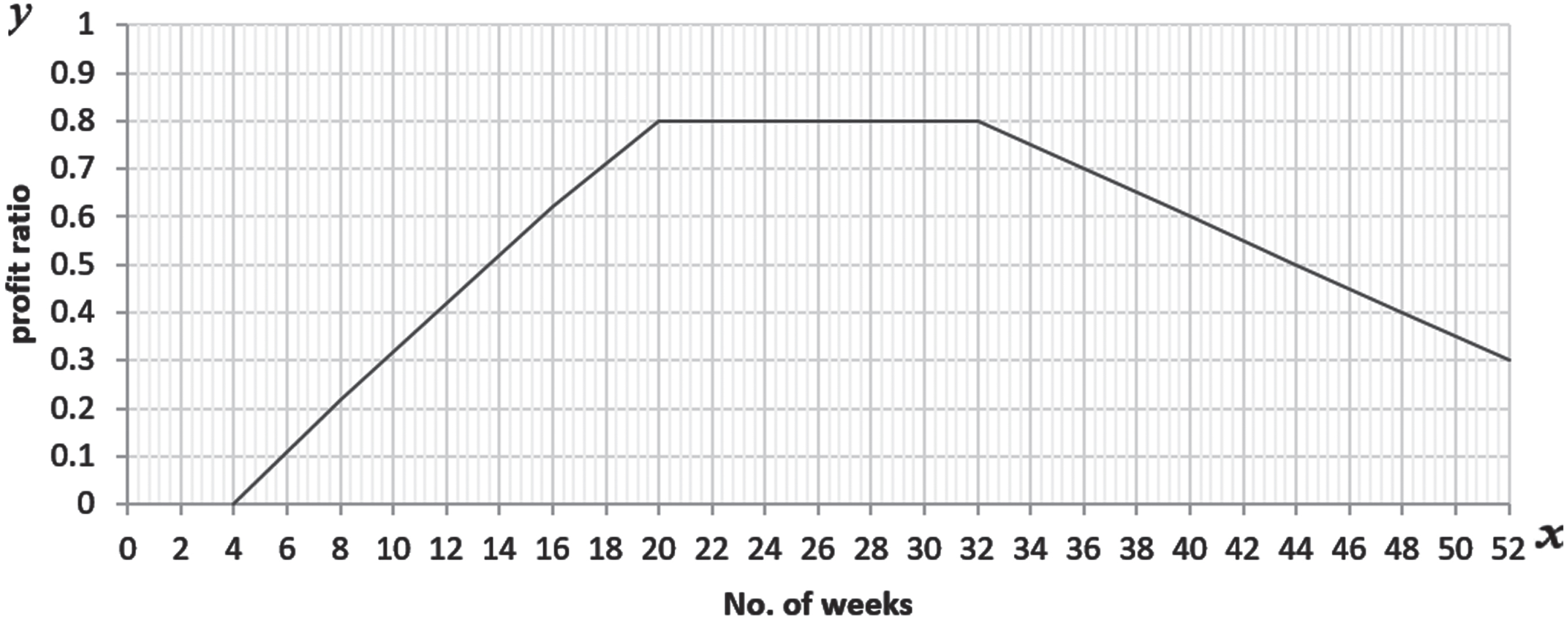
RLFRN.

5.3 Industry C

Industry C first made a fixed profit, which was then grown to a specific fixed sum and maintained for a specific amount of time. The profit was then reduced to a set sum at the conclusion of the time period. LFRN can be used to illustrate this circumstance. Let’s say that 10 lakhs is the monthly target profit for industry C.

Table 9 can be splinted into two types of tables where the contents of the Table 9 for x = 4,8,12,16,20 contribute Table 10 (Profit increasing type) and the contents of the Table 9 for x = 32, 36 … 52 contribute

Table 9

Monthly profit for Industry C

No. of weeks x	Profit	Profit ratio y
4	1000000	0
8	2000000	0.2
12	5000000	0.5
16	6000000	0.6
20	8000000	0.8
24	8000000	0.8
28	8000000	0.8
32	8000000	0.8
36	7000000	0.7
40	6000000	0.6
44	5000000	0.5
48	4000000	0.4
52	3000000	0.3

Table 10

Increasing pattern of profit for C

x i	y i
4	0.1
8	0.2
12	0.5
16	0.6
20	0.8

Table 11 (Profit decreasing type). In order to represent the data by a LFRNuse Regression formula to find the membership grades.

Table 11

Decreasing pattern of profit for C

x i	y i
32	0.8
36	0.7
40	0.6
44	0.5
48	0.4
52	0.3

Using Table 10 and the method which is discussed in section 5.1, the value of y in the interval [4, 20] is given by $y=0.045x-0.1=p\left(x\right)$

It can be verified that p(x) is increasing in the interval [4, 20].

Using Table 11 and the method which is discussed in section 5.1, the value of y in the interval [32, 52] is given by $y=-0.025x+1.6=q\left(x\right)$

It can be verified that q(x) is decreasing in the interval [32, 52].

Define $f_C\left(x\right)=\{\begin{array}{cc}0.8& 20⩽x⩽32\\ p\left(x\right)& 4⩽x⩽20\\ q\left(x\right)& 32⩽x⩽52\\ 0& \mathit{Otherwise}\\ \end{array}$

The graph of C is illustrated in Fig. 3.

Fig. 3

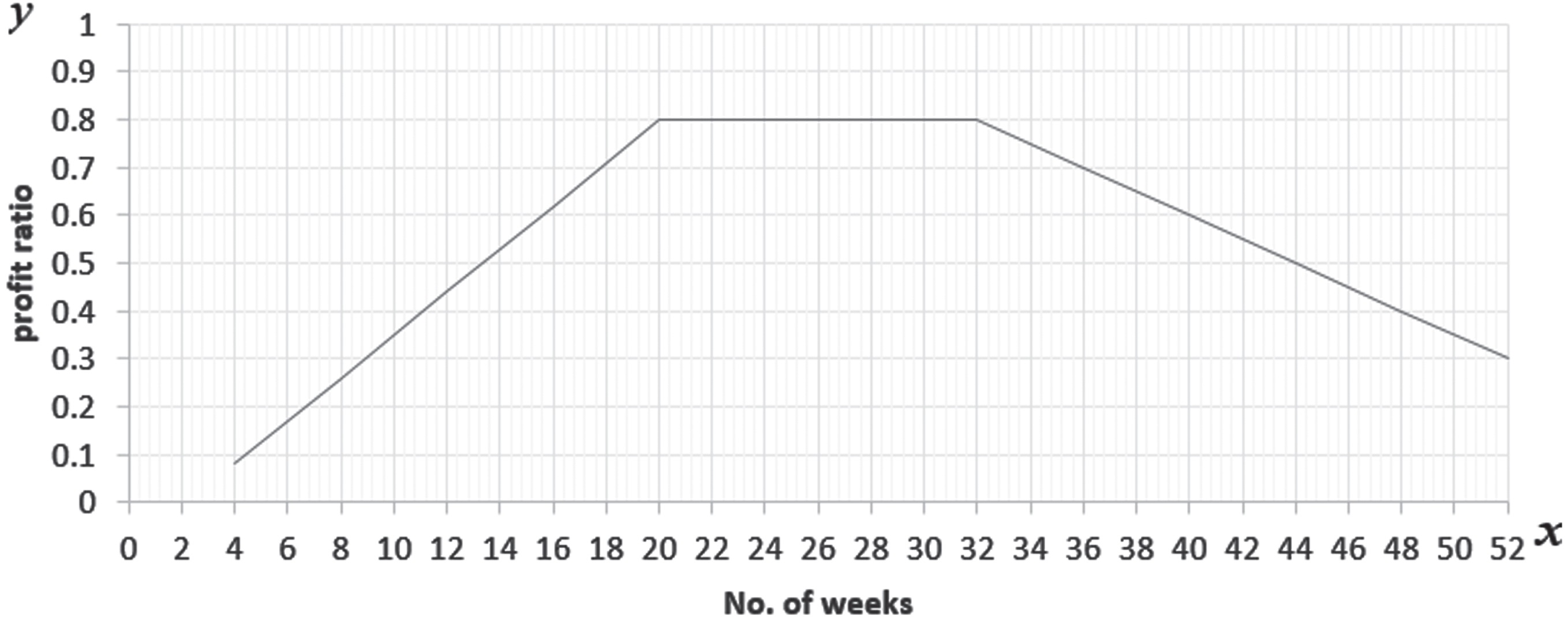
LFRN.

6 Advantages and disadvantages of the proposed fuzzy real number

6.1 Advantages

The advantage of the newly defined fuzzy real numbers is that they can represent data sets that cannot be represented by the current fuzzy numbers. The LLFRN, RLFRN, and LFRN metrics are being used to analyze data sets on daily prices for commodities like gold, silver, fuel etc. along with data sets on daily sales of such commodities during vacation periods or other noteworthy times in the current year. In a similar manner, data sets on a family’s, a company’s, or an organization’s income and expenditure can be analyzed utilizing LFRNs associated with the data sets, and the analysis over two separate times can be compared to determine the best course of action for income and expenditure. Fuzzy number theory is restricted to normalized fuzzy sets whereas this does not arise in the theory of LFRNs.

6.2 Disadvantages

Since the membership functions pertaining to the data set depend on the statistical tool used (e.g., regression line method, curve fitting method, parabolic curve fitting method, exponential curve fitting method, etc.), there are various techniques to represent the data set which are represented by LFRNs. LFRN theory analysis is limited to data sets that are separated into two groups, with the first group’s values showing a growing trend over one period and the second group’s values showing a decelerating trend over the following period. When the data set has numerous ups and downs over the period, the LFRNs cannot accurately represent the data set. The suggested fuzzy real numbers have limitations in that they can only be used with small data sets, making them unsuitable for big data sets.

7 Conclusion and further scope

In this study,three new types of fuzzy real numbers LLFRNs,RLFRNsand LFRNare introduced as generalizations of h-generalized fuzzy number. In order to demonstrate the applicability of the definitions of LLFRN, RLFRN, and LFRN, numerical examples and explanations were given. It is shown that every ɛ-cut of LFRNs is a closed interval and strong ɛ- cut of LFRNs can be either a closed interval or with the possibility of being a null interval. The representation of a real number by means of LFRNs, that of RLFRNs and that of LFRs also demonstrated. Every LFRN determines an LLFRN and RLFRN, which is an intriguing observation. A LFRN is also induced by a LLLFRN and a LRLFRN that have the same support, height, and core. As an application, the profit earned in the different types of industries are analyzed by LLFRN, RLFRN and LFRN models both analytically and graphically.

The LFRN theory may be extended to include the specific variants of fuzzy numbers and generalized fuzzy numbers such as triangular, trapezoidal, pentagonal, and hexagonal fuzzy numbers and their generic versions. Additionally, in the context of LFRN theory, fuzzy arithmetic, fuzzy similarity measures, fuzzy ranking systems, fuzzy decision-making approaches, and so on can be examined. If the mathematical operations on LFRNs are defined, a wider field of research will be produced in LFRN theory in comparison to the current fuzzy number theory, because LFRNs are suitable to analyze both non-normal and normalized fuzzy sets where as classic fuzzy real numbers can analyze normalized fuzzy sets only.