Fuzzy-Rough induced spectral ensemble clustering

Abstract

Ensemble clustering helps achieve fast clustering under abundant computing resources by constructing multiple base clusterings. Compared with the standard single clustering algorithm, ensemble clustering integrates the advantages of multiple clustering algorithms and has stronger robustness and applicability. Nevertheless, most ensemble clustering algorithms treat each base clustering result equally and ignore the difference of clusters. If a cluster in a base clustering is reliable/unreliable, it should play a critical/uncritical role in the ensemble process. Fuzzy-rough sets offer a high degree of flexibility in enabling the vagueness and imprecision present in real-valued data. In this paper, a novel fuzzy-rough induced spectral ensemble approach is proposed to improve the performance of clustering. Specifically, the significance of clusters is differentiated, and the unacceptable degree and reliability of clusters formed in base clustering are induced based on fuzzy-rough lower approximation. Based on defined cluster reliability, a new co-association matrix is generated to enhance the effect of diverse base clusterings. Finally, a novel consensus spectral function is defined by the constructed adjacency matrix, which can lead to significantly better results. Experimental results confirm that the proposed approach works effectively and outperforms many state-of-the-art ensemble clustering algorithms and base clustering, which illustrates the superiority of the novel algorithm.

1 Introduction

Clustering is an unsupervised learning method that usually refers to dividing existing unlabeled instances into several clusters according to the similarity between objects without any prior information, making the instances in the same cluster have a higher similarity and in different clusters have a more substantial discrepancy [9, 43]. Ensemble clustering utilises a consensus function to unify multiple types of partitions of the same dataset into one clustering result. It usually constructs a base clustering pool by repeatedly running a single clustering approach or executing multiple clustering algorithms. Then, the consensus function is built through voting methods, hypergraph partitioning, or evidence accumulation to obtain more optimal clustering results [18, 25]. Many existing ensemble clustering studies have confirmed that ensemble clustering can usually improve the clustering result compared to a single clustering algorithm [1, 24].

1.1 Background

Existing established clustering algorithms are mainly based on the theories of model, grid, density, partition, and hierarchy [2, 8]. Different types of clustering algorithms are good at solving diverse types, distributions, and scales of data. In particular, with the development of deep learning [27], the performance of various clustering methods has been further improved. For example, in [28], a deep-learning feature extractor for time-series data is designed for relation extraction, and the clustering effect achieved significant improvement. Nonetheless, in view of the unknown data distribution in actual problems, it is difficult to determine which clustering algorithm can get better clustering results. Conventional solutions often try different methods and choose the algorithm that performs best. Ensemble clustering is expected to establish a general scheme to combine the advantages of multiple clustering algorithms and form the optimal clustering result. It is especially feasible under the conditions of mature distributed computing technology, so as to adapt to unknown and complex data.

The related studies to ensemble clustering are mainly divided into three categories: pair-wise co-occurrence based, graph partitioning based, and median partition based algorithms [18]. The first type refers to constructing a co-occurrence matrix by finding the times of all instances that occur in pairs (assigned as a cluster) in base clusterings. The two instances should be classified into the same cluster in the final clustering based on co-occurrence [19]. The similarity function constructed by the co-occurrence matrix can be used in any similarity matrix based clustering algorithm to acquire the final optimal clustering result, such as hierarchical clustering and spectral clustering [7, 30]. The idea of co-occurrence matrix was first proposed in [5]. Correspondingly, a method of evidence accumulation clustering (EAC) based on this theory was proposed for the ensemble clustering problem. Subsequent researches have made various improvements, such as using the technique of normalised edges and matrix completion [29, 45]. In graph partitioning, the graph model and consensus function are usually constructed to partition the graph into multiple parts representing the final cluster. The primary purpose of graph partitioning is to achieve k-way min-cut partitioning, ensuring that the similarity between subgraphs is as tiny as possible [32]. Constructing a graph model is predominantly based on instances (vertices in hypergraph) or clusters (hyperedges in hypergraph) in base clustering. For example, the cluster-based similarity partitioning algorithm (CSPA) considers the local piecewise similarity and constructs a similarity graph as well as a graph partitioning method to perform ensemble clustering [23]. Compared with CSPA, the link-based ensemble clustering constructs a dense graph with the implied similarity between each instance and individual cluster; the clustering possesses a significant effect but needs too many computations [36]. The last type (median partition based algorithms) transforms ensemble clustering into an objective optimisation problem, which finds a median partition most similar to each base clustering by solving the objective function [17]. However, the issue is NP-hard [4]. Fortunately, some deconstructions, such as using expectation maximisation (EM) [40] and weighted consensus clustering (WCC) [33], have been proposed to find approximate solutions. In addition to the common types introduced above, ensemble algorithms based on voting [21], mutual information [20], finite mixture model [3] and other theories [22, 39] are also meaningful research directions in the field of ensemble clustering.

1.2 Motivations

Ensemble clustering is mainly divided into two steps. One is to generate a base clustering pool, for example, running the same clustering algorithm multiple times with different parameters, running various clustering algorithms multiple times, and performing clustering in subspaces. The other step is to select a consensus function, mainly based on the theories such as co-occurrence matrix, graph segmentation, and information entropy. An overview of ensemble clustering algorithms is depicted in Fig. 1.

Fig. 1

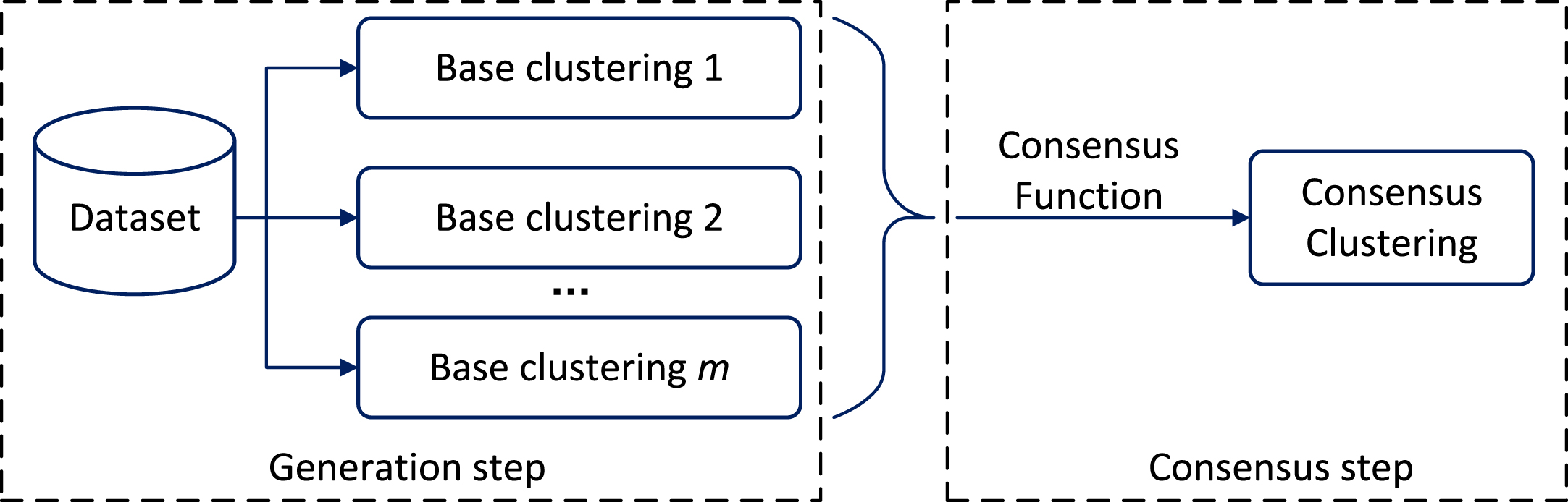
The outline of ensemble clustering.

In the numerous types of ensemble clustering solutions, the pair-wise co-occurrence based algorithms are pretty naive, easy to implement and have played a massive role in ensemble clustering fields. Nevertheless, these algorithms always treat all clusters in the base clustering equally, ignoring the difference of the clusters [35]. Some attempts have been used in cluster weighting to distinguish the effect of different clusters, such as weighting schemes of information entropy [14] and random walk [16]. The authors used related theories to distinguish different clusters and mine implicit relationships between instances. Corresponding experiments proved that it is effective to distinguish different clusters. However, these approaches always try to complete the ensemble clustering without the joining of features, but only the labels of base clusterings, which may lose some vital information implied in data features.

Fig. 2

The motivation of proposed method.

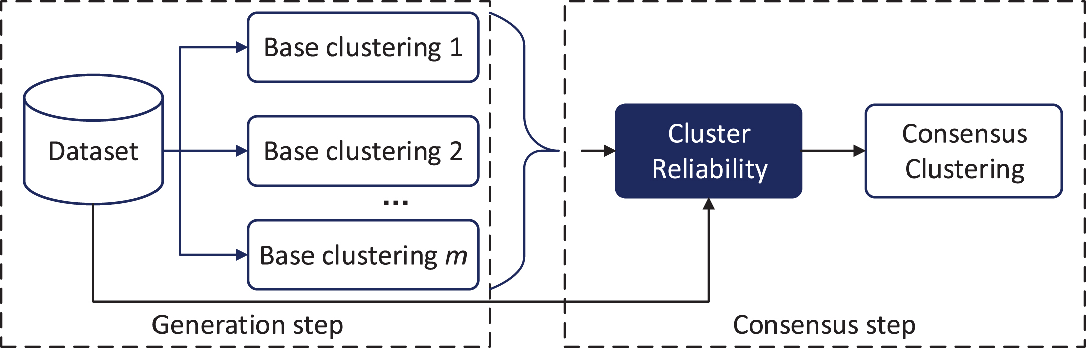
Compared with the algorithms considering base clustering results only, effectively combining base clustering and original features helps further improve the performance of ensemble clustering. Fuzzy-rough sets offer a high degree of flexibility in enabling the vagueness and imprecision present in real-valued data to be simultaneously modelled effectively [12, 38]. The idea of upper and lower approximation can well depict the membership of instances to each category, which is helpful for measuring the cluster reliability in ensemble clustering. The motivation of the proposed method is described in Fig. 2, and the solid black arrow and blue box are used to illustrate the difference with similar works, which means the joining of original features while distinguishing different cluster reliability.

1.3 Contributions

To distinguish the validity of different clusters and combine the role of features, in this paper, the fuzzy-rough lower approximation is used to induce cluster reliability in all base clusterings. A novel fuzzy-rough induced spectral ensemble clustering (FREC) algorithm is proposed to enhance the performance of pair-wise co-occurrence based ensemble clustering. The contribution of the paper is threefold:

Proposing the novel idea of cluster reliability through the fuzzy-rough lower approximation of each instance to enable the distinction of diverse cluster significance during clustering;

Developing a new adjacency matrix based on cluster reliability to effectively enhance the effect of diverse base clusterings and improve the clustering performance;

Establishing a consensus function and spectral ensemble clustering algorithm with its superiority confirmed through a comparative study and analysis on various benchmark datasets.

The experiment compares eleven state-of-the-art clustering algorithms on ten benchmark datasets, as well as the parallel algorithm that ignores the difference of clusters in base clustering. The result shows that FREC achieves a significant clustering performance. As the ensemble size increases, FREC achieves a superior effect.

The remainder of the paper is structured as follows. The preliminaries of the rough set and fuzzy-rough set are introduced in Section 2. The FREC algorithm is introduced in detail in Section 3. In Section 4, the experimental results are given and analysed. Finally, a summary is presented in Section 4.

2 Preliminaries

This section reviews the mathematical concepts concerning rough set and fuzzy-rough set, which are relevant to the reliability of the cluster developed in this paper.

2.1 Rough set

The study on rough sets theory [13, 49] provides a methodology that can be employed to extract knowledge from a domain in a concise way: it is able to minimise information loss whilst reducing the amount of information involved. Central to rough set theory is the concept of indiscernibility. Let $(U,A)$ be an information system, where $U$ is a set of instances and $A$ is a set of attributes (features) such that $a:U\to V_a$ for every $a\in A$ . V _a is the set of values that attribute a may take. For each feature subset $P\subseteq A$ , an associated P-indistinguishable relation can be determined: $\mathit{IND}\left(P\right)=\left\{\right(x,y)\in U^2\mid \forall a\in P,a(x)=a(y\left)\right\}.$(1)

Obviously, IND (P) is an equivalence relation on $U$ . The partition of $U$ determined by IND (P) is herein denoted by $U/P$ which can be defined such that $U/P=\otimes \{U/a|a\in P\}.$(2)

where ⊗ is defined as follows for sets V and W: $V\otimes W=\left\{X\cap Y|X\in V,Y\in W,X\cap Y\ne \varnothing \right\}.$(3)

For any object $x\in U$ , the equivalence class determined by IND (P), is denoted by [x]  _P . Let $X\subseteq U$ . X can be approximated using only the information contained in P by constructing the P-lower and P-upper approximations of X [48]: $\underset{\_}{P}X=\{x\mid [x{]}_P\subseteq X\},$(4) $\overline{P}X=\{x\mid [x{]}_P\cap X\ne \varnothing \}.$(5) The pair $〈\underset{\_}{P}X,\overline{P}X〉$ is called a rough set. Informally, the former depicts the set of those objects which can be said with certainty to belong to the concept approximated, and the latter is the set of objects which either definitely or possibly belong to the concept approximated. The difference between the upper and lower approximations is the area known as the boundary region that represents the area of uncertainty. If the boundary region is empty, there is no uncertainty regarding the concept which is being approximated and all objects belong to the subset of objects of interest with full certainty.

2.2 Fuzzy-rough set

Fuzzy-rough sets [6, 38] encapsulate the related but distinct concepts of vagueness (for fuzzy sets) and indiscernibility (for rough sets), both of which occur as a result of uncertainty in knowledge. Compared to rough sets, fuzzy-rough sets offer a high degree of flexibility in enabling the vagueness and imprecision present in real-valued data to be simultaneously modelled effectively. In fuzzy-rough sets, the fuzzy lower and upper approximations to approximate a fuzzy concept X can be defined as: ${\mu }_{\underset{\_}{R_P}X}\left(x\right)=\underset{y\in U}{inf}\mathcal{I}\left({\mu }_{R_P}\right(x,y),{\mu }_X(y\left)\right),$(6) ${\mu }_{\overline{R_P}X}\left(x\right)=\underset{y\in U}{sup}\mathcal{T}\left({\mu }_{R_P}\right(x,y),{\mu }_X(y\left)\right).$(7)

Here, $\mathcal{I}$ is a fuzzy implicator and $\mathcal{T}$ is a T-norm. R _P is a T-transitive fuzzy similarity relation induced by the subset of features P: ${\mu }_{R_P}(x,y)={\mathcal{T}}_{a\in P}\left\{{\mu }_{R_a}\right(x,y\left)\right\},$(8) where μ _{R a}  (x, y) is the degree to which object x and y are similar for feature a, and may be defined in many ways, for example: ${\mu }_{R_a}(x,y)=exp\left(-\frac{\left(a\right(x)-a(y){)}^2}{2{{\sigma }_a}^2}\right),$(9) $\begin{array}{cc}\hfill {\mu }_{R_a}(x,y)=& max(min(\frac{\left(a\right(y)-(a\left(x\right)-{\sigma }_a\left)\right)}{\left(a\right(x)-(a\left(x\right)-{\sigma }_a\left)\right)},\hfill \\ \hfill & \frac{\left(\right(a\left(x\right)+{\sigma }_a)-a(y\left)\right)}{\left(\right(a\left(x\right)+{\sigma }_a)-a(x\left)\right)}),0).\hfill \end{array}$(10) Same as their crisp parallels, ${\mu }_{\underset{\_}{R_P}X}\left(x\right)$ and ${\mu }_{\overline{R_P}X}\left(x\right)$ indicate the degrees to which the object x must and may belong to the approximated fuzzy concept X, respectively.

3 Fuzzy-rough induced spectral ensemble clustering

3.1 The unacceptable degree of clusters

The validity of a cluster can be well judged by considering the unacceptable degree (UD) of clusters in a base clustering. In multiple base clusterings, if the assignment of a cluster in one base clustering is consistently agreed by other base clusterings, this cluster should play a more critical role in the final consensus clustering. At the same time, if the assignment of a cluster is constantly negated by other base clusterings, the cluster should play a minor role.

For illustration purposes, some formalised descriptions are first introduced below. Let $U=\left\{x_i\right|i\in 1,2,...,n\}$ be an instances set, x _i is an instance which contains d features. B = {β _j |j ∈ 1, 2, . . . , m} is a set of base clusterings where ${\beta }_j=\left\{{\beta }_j^k\right|k\in 1,2,...,K\}$ indicates the instances set in the k-th cluster of the j-th base clustering. The degree of x _i belongs to ${\beta }_j^k$ with the features set $A$ can be calculated by the fuzzy lower approximation ${\mu }_{\underset{\_}{R_A}{\beta }_j^k}\left(x_i\right)$ .

Since for every fuzzy implicator $\mathcal{I}$ , there is $\mathcal{I}(\mathcal{x},1)=1$ , ${\mu }_{\underset{\_}{R_A}{\beta }_j^k}\left(x_i\right)$ can be simplified into:

$\begin{array}{cc}\hfill & {\mu }_{\underset{\_}{R_A}{\beta }_j^k}\left(x_i\right)\hfill \\ \hfill =& \underset{y\in U}{inf}\mathcal{I}\left({\mu }_{R_A}\right(x_i,y),{\mu }_{{\beta }_j^k}(y\left)\right)\hfill \\ \hfill =& min\{\underset{y\in {\beta }_j^k}{min}\left\{\mathcal{I}\left({\mu }_{R_A}\left(x_i,y\right),1\right)\right\},\hfill \\ \hfill & \underset{y\notin {\beta }_j^k}{min}\left\{\mathcal{I}\left({\mu }_{R_A}\left(x_i,y\right),0\right)\right\}\}\hfill \\ \hfill =& \underset{y\notin {\beta }_j^k}{min}\left\{\mathcal{I}\left({\mu }_{R_A}\left(x_i,y\right),0\right)\right\}.\hfill \end{array}$(11)

As proved in [31], if $\mathcal{I}$ belongs to S-implications, QL-implications or R-implications which enjoys contrapositive symmetry, it is that $\mathcal{I}(\mathcal{x},0)=\mathcal{N}\left(\mathcal{x}\right)$ , where $\mathcal{N}$ is the strong negator to induce $\mathcal{I}$ . In particular, for the classical strong negation ${\mathcal{N}}_{\mathcal{C}}\left(\mathcal{x}\right)=1-\mathcal{x}$ , Equation (11) can be further modified to:

$\begin{array}{cc}\hfill {\mu }_{\underset{\_}{R_A}{\beta }_j^k}\left(x_i\right)& =\underset{y\notin {\beta }_j^k}{min}\left\{1-\left({\mu }_{R_A}\left(x_i,y\right)\right)\right\}\hfill \\ \hfill & =1-\underset{y\notin {\beta }_j^k}{max}\left\{{\mu }_{R_A}\left(x_i,y\right)\right\}.\hfill \end{array}$(12)

Equation (12) implies that the lower approximation of x _i to ${\beta }_j^k$ depends on the most similar instance in different clusters, which has a crucial role in ensemble clustering. It indicates that the farther the two clusters are, the greater the lower approximation of each instance to the cluster to which it belongs. At the same time, it means that the distinction between clusters is more obvious, that is, the cluster allocation scheme is more reasonable.

For different base clusterings, the assignment of clusters is distinct, but the data location is fixed, that is, multiple base clusterings are acting on the same dataset. For a specific cluster in one base clustering, the resulting assignment has two cases:

Another base clustering approves this assignment;

Another base clustering denies this assignment.

In this paper, a novel concept of UD is proposed to metric the cluster reliability. Here, two exemplar artificial datasets D1 (shown in Fig. 3) and D2 (shown in Fig. 4) are employed to illustrate the UD of the two cases.

Fig. 3

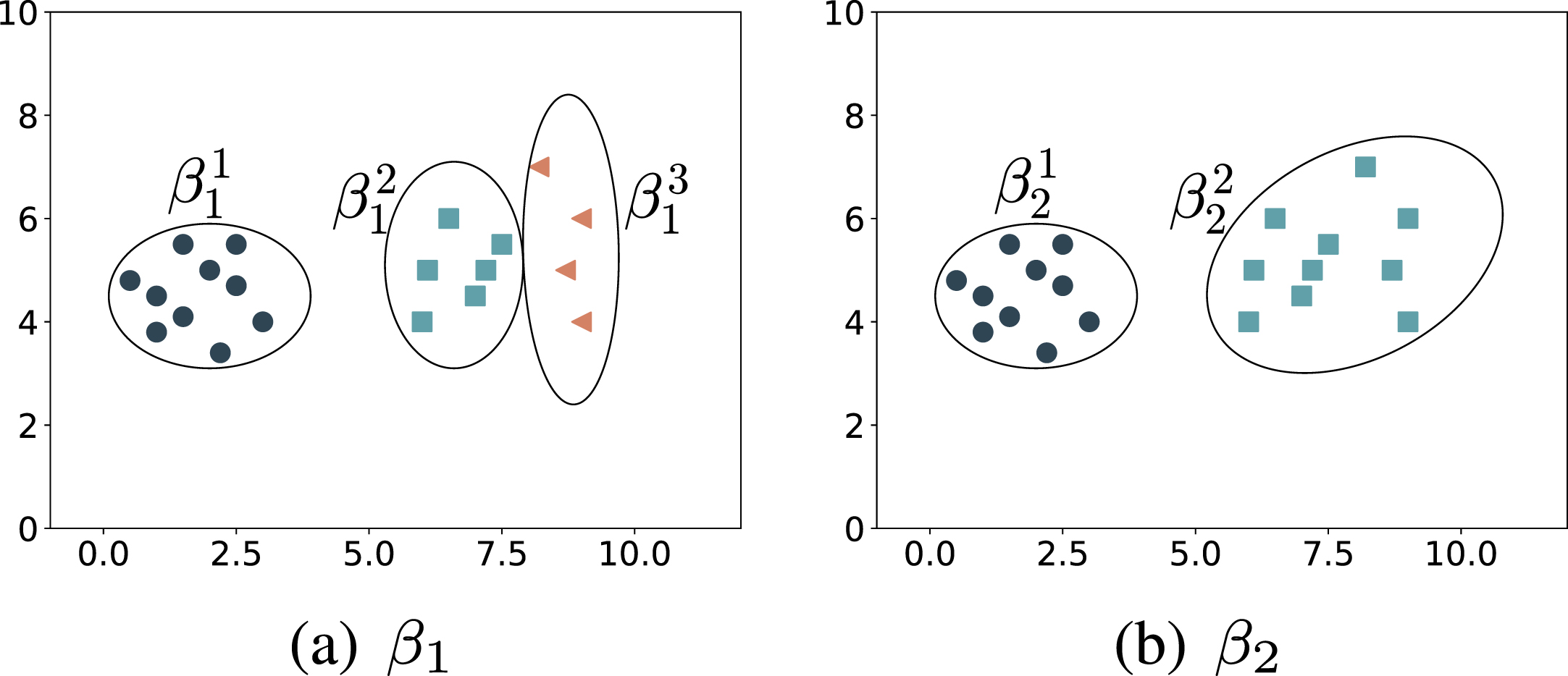
Two exemplar base clusterings β₁ and β₂ in dataset D1.

The first case is relatively simple, as shown in Fig. 3, including two exemplar base clusterings β₁ and β₂ in D1. For a specifically given cluster (e.g., ${\beta }_1^1$ ) in base clustering β₁, considering the distribution of this cluster in another base clustering β₂, an obvious fact is that if the particular cluster in β₁ is a subset of one cluster in β₂, the assignment of the cluster (e.g. ${\beta }_1^1$ ) can be considered to be fully admitted by β₂. At this point, the UD of the specific cluster in β₁ is 0, which means that the objects of the cluster in β₁ meeting the above condition can be divided into one cluster in both base clustering β₁ and β₂.

For the three clusters ( ${\beta }_1^1$ , ${\beta }_1^2$ , ${\beta }_1^3$ ) of β₁ shown in Fig. 3(a), considering the base clustering β₂, ${\beta }_1^1$ is a subset of ${\beta }_2^1$ , and both ${\beta }_1^2$ and ${\beta }_1^3$ are subsets of ${\beta }_2^2$ , so the UD is 0 for all three clusters in β₁. It is worth noting that this relationship is not symmetric, that is, the clusters in β₁ are admitted by β₂, which does not mean that the clusters in β₂ are admitted by β₁.

Another situation is shown in Fig. 4. For a particular cluster in β₃, if the cluster objects are split into a plurality of clusters in another base clustering β₄, it can be considered that the specific cluster is not admitted or accepted by β₄. Here, ${\beta }_3^1$ is split into ${\beta }_4^1$ and ${\beta }_4^2$ by β₄, and ${\beta }_3^2$ is split into ${\beta }_4^3$ and ${\beta }_4^4$ by β₄, which means β₄ disagrees with the allocation of ${\beta }_3^1$ and ${\beta }_3^2$ . Further, the UD can be well measured by the lower approximation of cluster objects in β₃ to the base clustering β₄.

Fig. 4

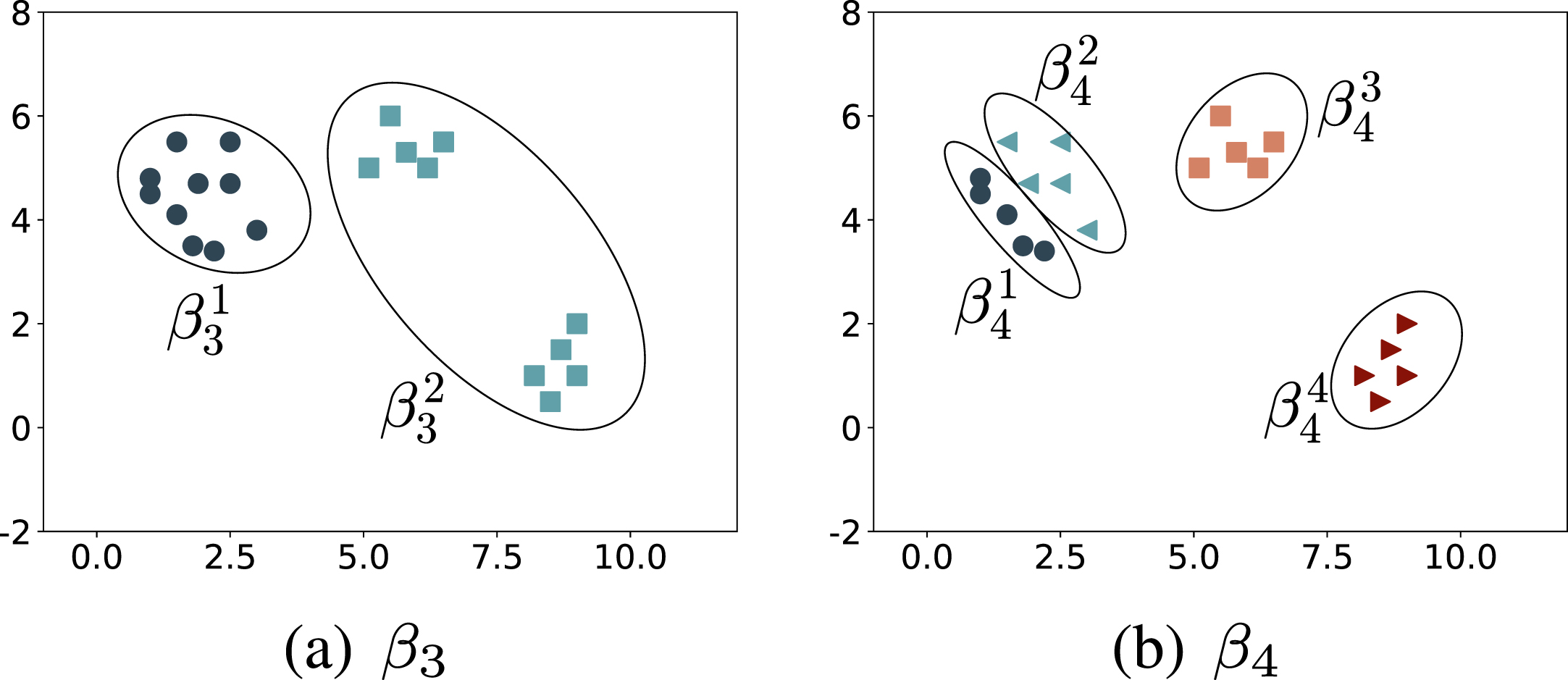
Two exemplar base clusterings β₃ and β₄ in dataset D2.

More specifically, for a specific cluster in a base clustering, considering its position distribution in another base clustering, if the objects of this particular cluster have a more significant lower approximation to the cluster in which the objects relocate in another base clustering, it indicates that the given cluster prefers the allocation of another base clustering. At the same time, it also means the extent of another base clustering does not accept the assignment of the given cluster.

Objects from ${\beta }_j^k$ may be located in one or multiple clusters in another base clustering β _l , such indeterminate clusters can be represented by $R_{\mathit{jl}}^k=\left\{{\beta }_l^s\right|{\beta }_j^k\cap {\beta }_l^s\ne \varnothing ,{\beta }_l^s\in {\beta }_l\},l\ne j$(13)

For the example cluster ${\beta }_3^1$ in Fig. 4(a), the set $R_{34}^1$ is { ${\beta }_4^1,{\beta }_4^2$ }. Based on the analysis above, the UD ${\gamma }_{\mathit{jl}}^k$ of the cluster ${\beta }_j^k$ relative to another base clustering β _l can be defined as: ${\gamma }_{\mathit{jl}}^k=\{\begin{array}{cc}0,\hfill & \left|R_{\mathit{jl}}^k\right|=1,\hfill \\ \frac{1}{\left|{\beta }_j^k\right|}\sum _{{\beta }_l^s\in R_{\mathit{jl}}^k}\sum _{x_i\in {\beta }_j^k\cap {\beta }_l^s}{\mu }_{\underset{\_}{R_A}{\beta }_l^s}\left(x_i\right),\hfill & \left|R_{\mathit{jl}}^k\right|>1.\hfill \\ \hfill & \hfill \end{array}$(14) where $\left|R_{\mathit{jl}}^k\right|$ indicates the number of the clusters in set $\left|R_{\mathit{jl}}^k\right|$ , and $\left|{\beta }_j^k\right|$ represents the number of the instances in ${\beta }_j^k$ .

To illustrate the concepts involved, the objects of the exemplar clusters ${\beta }_3^1$ and ${\beta }_3^2$ in Fig. 4(a) are given in Table 1, the relocated clusters in β₄ are recorded in Table 2.

Table 1

Two exemplar clusters in Fig. 4(a)

Cluster	Sample	x 1	x 2	x 3	x 4	x 5	x 6	x 7	x 8	x 9	x 10
${\beta }_3^1$	x-axis	1.0	1.0	1.5	2.2	1.8	1.9	2.5	1.5	2.5	3.0
	y-axis	4.5	4.8	4.1	3.4	3.5	4.7	4.7	5.5	5.5	3.8
Cluster	Sample	x 11	x 12	x 13	x 14	x 15	x 16	x 17	x 18	x 19	x 20
${\beta }_3^2$	x-axis	5.8	5.1	5.5	6.2	6.5	8.2	9.0	8.7	8.5	9.0
	y-axis	5.3	5.0	6.0	5.0	5.5	1.0	2.0	1.5	0.5	1.0

Table 2

Relocated cluster of the objects in ${\beta }_3^1$ and ${\beta }_3^2$

Sample ( ${\beta }_3^1$ )	x 1	x 2	x 3	x 4	x 5	x 6	x 7	x 8	x 9	x 10
Relocated cluster	${\beta }_4^1$					${\beta }_4^2$
Sample ( ${\beta }_3^2$ )	x 11	x 12	x 13	x 14	x 15	x 16	x 17	x 18	x 19	x 20
Relocated cluster	${\beta }_4^3$					${\beta }_4^4$

Take x₁, x₆, x₁₁ and x₁₆ as an example (located in diverse clusters in β₄), the respective lower approximation of the above four objects to β₄ are obtained by using the Algebraic T-norm ${\mathcal{T}}_{\mathcal{P}}(\mathcal{a},\mathcal{b})=\mathcal{ab}$ and the fuzzy similarity function (9): $\begin{array}{cc}\hfill & x_1\in {\beta }_4^1\Rightarrow {\mu }_{\underset{\_}{R_A}{\beta }_4^1}\left(x_1\right)=0.05,\hfill \\ \hfill & x_6\in {\beta }_4^2\Rightarrow {\mu }_{\underset{\_}{R_A}{\beta }_4^2}\left(x_6\right)=0.05,\hfill \\ \hfill & x_{11}\in {\beta }_4^3\Rightarrow {\mu }_{\underset{\_}{R_A}{\beta }_4^3}\left(x_{11}\right)=0.91,\hfill \\ \hfill & x_{16}\in {\beta }_4^4\Rightarrow {\mu }_{\underset{\_}{R_A}{\beta }_4^4}\left(x_{16}\right)=0.94.\hfill \end{array}$

Through further calculations, the lower approximation of all objects in β₃ to the base clustering β₄ are shown in Table 3.

Table 3

Lower approximation of ${\beta }_3^1$ and ${\beta }_3^2$ to the base clustering β₄

Cluster	Relocation	x 1	x 2	x 3	x 4	x 5	x 6	x 7	x 8	x 9	x 10
${\beta }_3^1$	${\beta }_4^1$	0.05	0.05	0.07	0.06	0.10	-	-	-	-	-
	${\beta }_4^2$	-	-	-	-	-	0.05	0.11	0.10	0.19	0.07
Cluster	Relocation	x 11	x 12	x 13	x 14	x 15	x 16	x 17	x 18	x 19	x 20
${\beta }_3^2$	${\beta }_4^3$	0.91	0.90	0.96	0.86	0.91	-	-	-	-	-
	${\beta }_4^4$	-	-	-	-	-	0.94	0.86	0.91	0.97	0.95

Then, the UD of ${\beta }_3^1$ and ${\beta }_3^2$ to base clustering β₄ is computed by Equation (14), there is $\begin{array}{cc}\hfill {\gamma }_{34}^1& =\frac{0.05+0.05+0.07+0.06+0.10+0.05+0.11+0.10+0.19+0.07}{10}\hfill \\ \hfill & =0.09\hfill \\ \hfill {\gamma }_{34}^2& =\frac{0.91+0.90+0.96+0.86+0.91+0.94+0.86+0.91+0.97+0.95}{10}\hfill \\ \hfill & =0.92\hfill \end{array}$

Considering the ground distribution of ${\beta }_3^1$ and ${\beta }_3^2$ in Fig. 4, apparently, the allocation scheme of ${\beta }_3^1$ is more reasonable, with a lower UD of 0.09. While ${\beta }_3^2$ groups the objects with an enormous difference, the UD is 0.92. The result shows that the UD acquired is consistent with the actual situation of the clusters.

Further, the global UD ${\gamma }_j^k$ of a cluster in β _j to the remaining m - 1 base clustering can be calculated as follows: ${\gamma }_j^k=\frac{1}{m-1}\sum _{l\ne j}{\gamma }_{\mathit{jl}}^k,l=1,2,...,m.$(15)

The unacceptable degree computing (UDC) algorithm is outlined in Algorithm 1. Given the inputs $U$ and m, the first step is to initialise the set Γ empty and generate m base clusterings by any constructed method, such as repeating k-means m times and using diverse results from multiple clustering algorithms [34]. The loop in Lines 3 to 14 traverses each cluster in all base clusterings and computes the UD. Specifically, ${\beta }_j^k$ represents the current cluster to calculate UD, and β _l indicates any cluster in the base clusterings set except β _j . Mean(·) defines an average process, and all computed UD is stored in Γ. Finally, in Line 15, the Γ is returned for subsequent calculations.

Algorithm 1

Unacceptable Degree Computing (UDC)

UDC ( $U$ , m)

Input:

   $U$ , input space containing n objects,

  m, number of base clusterings.

Output:

  Γ, set of unacceptable degree of all clusters,

  B, set of base clusterings.

1:  Initialise: Γ = ∅.

2:  B ← Generate m base clustering.

3:  foreach β _j in B do

4:   foreach ${\beta }_j^k$ in β _j do

5:    S = ∅

6:    foreach β _l in {B - β _j } do

7:      $R_{\mathit{jl}}^k$ ← Equation (13)

8:      ${\gamma }_{\mathit{jl}}^k$ ← Equation (14)

9:     S = S ∪ ${\gamma }_{\mathit{jl}}^k$

10:    end

11:     ${\gamma }_j^k$ = Mean(S)

12:    Γ = $\Gamma \cup {\gamma }_j^k$

13:   end

14:  end

15:  return Γ, B

3.2 Defining the co-association matrix

Fig. 5

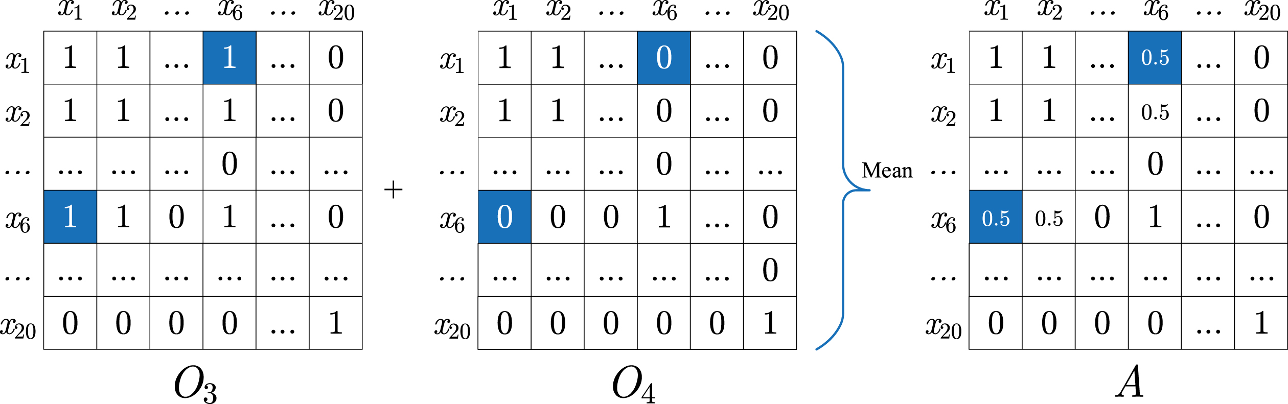
Matrices O₃, O₄ and A of the example in Fig. 4.

Fig. 6

Redefined Matrices ${\tilde{O}}_3$ , ${\tilde{O}}_4$ and $\tilde{A}$ of the example in Fig. 4.

The co-association matrix is obtained by summing and averaging a series of co-occurrence matrices, and it represents the frequency with which two objects co-occur in multiple base clusterings. Each base clustering β _j produces a separate co-occurrence matrix, which can be expressed as

$O_j=\{o_{\mathit{ih}}^j{\}}_{n\times n},$(16) where $o_{\mathit{ih}}^j$ represents whether x _i and x _h co-occur in β _j . Let C _j  (x _i ) indicate the serial number of the cluster to which x _i belongs in the j-th base clustering, $o_{\mathit{ih}}^j$ can be denoted by $\begin{array}{c}\hfill o_{\mathit{ih}}^j=\{\begin{array}{cc}1,\hfill & C_j\left(x_i\right)=C_j\left(x_h\right),\hfill \\ 0,\hfill & C_j\left(x_i\right)\ne C_j\left(x_h\right).\hfill \end{array}\end{array}$(17) Further, the co-association matrix can be expressed as

$A=\{a_{\mathit{ih}}{\}}_{n\times n},$(18) where a _ih is calculated by $a_{\mathit{ih}}=\frac{1}{m}\sum _{j=1}^m{o}_{\mathit{ih}}^j.$(19)

Given the exemplar clusters in Fig. 4 and corresponding coordinates in Table 1, the matrices O₃, O₄ and A are recorded in Fig. 5. Take x₁ and x₆ as an example (marked as a blue box): $\begin{array}{cc}\hfill & C_3\left(x_1\right)=C_3\left(x_6\right)\Rightarrow o_{16}^3=1,o_{61}^3=1,\hfill \\ \hfill & C_4\left(x_1\right)\ne C_4\left(x_6\right)\Rightarrow o_{16}^4=0,o_{61}^4=0.\hfill \end{array}$

Then, the elements a₁₆ and a₆₁ of A are calculated by $\begin{array}{cc}\hfill & o_{16}^3=1,o_{16}^4=0\Rightarrow a_{16}=(1+0)/2=0.5,\hfill \\ \hfill & o_{61}^3=1,o_{61}^4=0\Rightarrow a_{61}=(1+0)/2=0.5.\hfill \end{array}$

A higher UD for a cluster indicates that other base clusterings are more likely to disapprove of the cluster’s allocation scheme. At this point, the role of the cluster should be weakened. Otherwise, the function of the cluster should be reinforced. Therefore, the reliability of a cluster can be described as a decreasing function of the UD. In this paper, the reliability of the k-th cluster in β _j is defined as ${\mu }_j^k=1-{\gamma }_j^k.$(20)

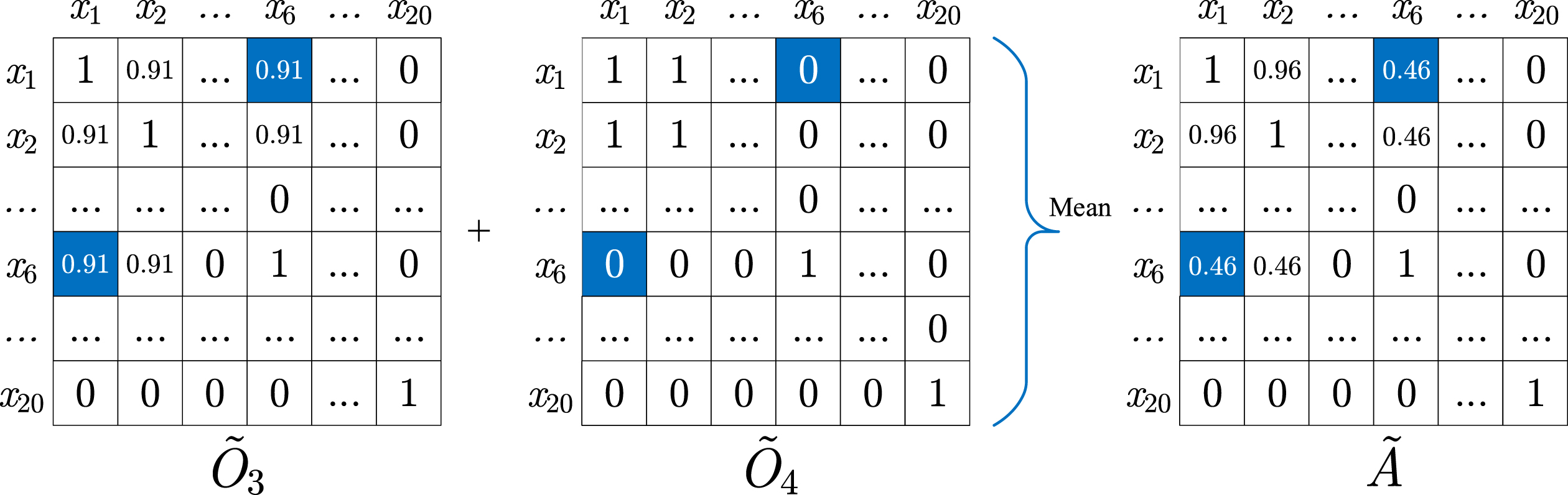
Similar to Equations (16), (18) and (19), the redefined co-occurrence matrix ${\tilde{O}}_j$ and co-association matrix $\tilde{A}$ are expressed as

${\tilde{O}}_j=\{{\tilde{o}}_{\mathit{ih}}^j{\}}_{n\times n},$(21)

$\tilde{A}=\{{\tilde{a}}_{\mathit{ih}}{\}}_{n\times n},$(22) where $\begin{array}{cc}\hfill {\tilde{o}}_{\mathit{ih}}^j=\{\begin{array}{cc}{\mu }_j^k,\hfill & C_j\left(x_i\right)=C_j\left(x_h\right),\hfill \\ 0,\hfill & C_j\left(x_i\right)\ne C_j\left(x_h\right).\hfill \\ \parallel \hfill & \hfill \end{array}& \hfill \end{array}$(23) ${\tilde{a}}_{\mathit{ih}}=\frac{1}{m}\sum _{j=1}^m{\tilde{o}}_{\mathit{ih}}^j.$(24)

Again, for the example of x₁ and x₆, $\begin{array}{cc}\hfill & C_3\left(x_1\right)=C_3\left(x_6\right)\Rightarrow {\tilde{o}}_{16}^3=0.91,{\tilde{o}}_{61}^3=0.91,\hfill \\ \hfill & C_4\left(x_1\right)\ne C_4\left(x_6\right)\Rightarrow {\tilde{o}}_{16}^4=0,{\tilde{o}}_{61}^4=0.\hfill \end{array}$

Then, the elements ${\tilde{a}}_{16}$ and ${\tilde{a}}_{61}$ of $\tilde{A}$ are computed by $\begin{array}{cc}\hfill \begin{array}{c}{\tilde{o}}_{16}^3=0.91\\ {\tilde{o}}_{16}^4=0\\ \end{array}\}& \Rightarrow {\tilde{a}}_{16}=(0.91+0)/2=0.46,\hfill \\ \hfill \begin{array}{c}{\tilde{o}}_{61}^3=0.91\\ {\tilde{o}}_{61}^4=0\\ \end{array}\}& \Rightarrow {\tilde{a}}_{61}=(0.91+0)/2=0.46.\hfill \end{array}$

The matrices ${\tilde{O}}_3$ , ${\tilde{O}}_4$ and $\tilde{A}$ of the exemplar clusters in Fig. 4 are recalculated and shown in Fig. 6.

Algorithm 2

Co-Association Matrix Construction (CMC)

CMC ( $U$ , Γ, B)

Input:

$U$ , input space containing n objects,

  Γ, set of unacceptable degree of all clusters,

  B, set of base clusterings.

Output: $\tilde{A}$ , co-association matrix.

1:  Initialise:    $\tilde{A}=\left\{{\tilde{a}}_{\mathit{ih}}{\}}_{n\times n}\right({\tilde{a}}_{\mathit{ih}}=1),{\tilde{O}}_j=\{{\tilde{o}}_{\mathit{ih}}^j{\}}_{n\times n}({\tilde{o}}_{\mathit{ih}}^j=0)$ .

2:  foreach i = 1 to n do

3:   foreach h = i + 1 to n do

4:    Q = ∅

5:    foreach β _j in B do

6:     if C _j  (x _i ) ≠ C _j  (x _h ) then ${\tilde{o}}_{\mathit{ih}}^j$ = 0

7:     else

8:      k = C _j  (x _i )

9:       ${\mu }_j^k$ = $1-{\gamma }_j^k$

10:       ${\tilde{o}}_{\mathit{ih}}^j$ = ${\mu }_j^k$

11:     end

12:     Q = Q ∪ ${\tilde{o}}_{\mathit{ih}}^j$

13:    end

14:     ${\tilde{a}}_{\mathit{ih}}$ = Mean(Q)

15:     ${\tilde{a}}_{\mathit{hi}}$ = ${\tilde{a}}_{\mathit{ih}}$

16:   end

17:  end

18:  return $\tilde{A}$

The co-association matrix construction (CMC) algorithm is detailed in Algorithm 2. Firstly, the initialised step is performed. Lines 2 to 17 represent the overall process, including the main loop to identify the co-occurrence and co-association matrices. Note that all matrices are calculated only for upper triangular due to the symmetry. In Line 15, the lower triangular matrix of $\tilde{A}$ directly takes the values from the existing result in Line 14, which can significantly diminish unnecessary calculations. The final co-association matrix $\tilde{A}$ is output in Line 18.

3.3 Consensus function

A mapping from a set of clusterings to a single final clustering is called a consensus function. Considering the superior performance of spectral clustering in complex shapes and cross data, in this paper, the optimised co-association matrix is used in the spectral method to acquire the consensus result.

Given a graph model G = (V, L), where V indicates the vertexes set and L represents the links set. Its adjacency matrix can be constructed in various ways, such as considering the neighbours or defining the distance threshold. Let the objects in $U$ be the vertexes in the graph, the adjacency matrix can be expressed as $\tilde{A}$ . It means that if a _ih is 0, there is no edge connection between x _i and x _h . Otherwise, the edge exists and the similarity is a _ih . From this, the diagonal matrix D can be expressed by

$D=\{d_{\mathit{ih}}{\}}_{n\times n},$(25) where $\begin{array}{cc}\hfill d_{\mathit{ih}}=\{\begin{array}{cc}0,\hfill & i\ne h,\hfill \\ \sum _{q=1}^n{\tilde{a}}_{\mathit{iq}},\hfill & i=h.\hfill \\ \hfill & \hfill \end{array}& \hfill \end{array}$(26)

The Laplacian matrix L of the graph G can be further defined as

$L=D-\tilde{A}.$(27)

Normalisation makes the diagonal entries of the Laplacian matrix to be all units and scales off-diagonal entries correspondingly. In this case, the normalised Laplacian matrix L _nor is defined as

$L_{\mathit{nor}}=D^{-\frac{1}{2}}{\mathit{LD}}^{-\frac{1}{2}}.$(28)

The components of the eigenvectors corresponding to the smallest eigenvalues of the graph Laplacian can be used for meaningful clustering [42]. In Equation (28), the eigenvectors corresponding to the first K smallest eigenvalues of L _nor will be used in an independent clustering algorithm, generally k-means, due to its speed and efficiency.

As summarised in Algorithm 3, D and L _nor are computed sequentially in Lines 2 to 6. EV(·) in Line 7 represents a function that generates the first K eigenvectors, and k-means(·) in Line 8 indicates a fast clustering algorithm detailed in [34]. Finally, in Line 9, $\mathcal{R}$ is used to return the consensus clustering result.

Algorithm 3

Consensus Spectral Clustering (CSC)

CSC ( $\tilde{A}$ , K)

Input:

   $\tilde{A}$ , co-association matrix,

  K, number of clusters.

Output: $\mathcal{R}$ , consensus result.

1:  Initialise: D = {d _ih } _n×n (d _ih  = 0) .

2:  foreach i = 1 to n do

3:   d _ii = ${\sum }_{q=1}^n{\tilde{a}}_{\mathit{iq}}$

4:  end

5:   $L=D-\tilde{A}$

6:   $L_{\mathit{nor}}=D^{-\frac{1}{2}}{\mathit{LD}}^{-\frac{1}{2}}$

7:  F← EV(L _nor )

8:   $\mathcal{R}\leftarrow$ k-means(F, K)

9:  return $\mathcal{R}$

3.4 Fuzzy-rough induced spectral ensemble clustering

According to the description of the above three subsections, the overall fuzzy-rough induced spectral ensemble clustering is depicted in Algorithm 4. Given a dataset $U$ , the number of base clusterings m and the actual clusters number K. Algorithm 1 is first executed to generate the UD set Γ of all clusters and the set of base clusterings B in Line 1. Further, the result returned by Algorithm 1 is combined with the dataset $U$ as the parameters of Algorithm 2 to calculate the co-association matrix $\tilde{A}$ . Finally, the matrix $\tilde{A}$ is used in the consensus spectral clustering (CSC) to generate the final clustering result $\mathcal{R}$ .

Algorithm 4

Fuzzy-Rough Induced Spectral Ensemble Clustering (FREC)

FREC ( $U$ , m, K)

Input:

   $U$ , input space containing n objects,

  m, number of base clusterings,

  K, number of clusters.

Output: $\mathcal{R}$ , consensus result.

1: Γ, B = UDC( $U$ , m) //Algorithm 1

2:  $\tilde{A}$ = CMC( $U$ , Γ, B) //Algorithm 2

3:  $\mathcal{R}$ = CSC( $\tilde{A}$ , K) //Algorithm 3

4: return $\mathcal{R}$

4 Experimental evaluation

This section presents the experimental evaluation of FREC and other algorithms on ten popular datasets contained in UCI 1 repository. For convenience, datasets Cardiotocography, Image Segmentation, and Steel Plates Faults are represented by abbreviations Cardio, IS, and SPF, respectively. After introducing the experimental setup, the results and discussion are divided into five parts. Section 4.2 analyses the tendency of clustering effect as the number of ensembles increases. To test the impact of cluster reliability induced by fuzzy-rough lower approximation, Section 4.3 compares the effect of FREC and the original parallel algorithm EAC on all benchmark datasets. Besides, the average result of 100 base clusterings is also used to compare and validate the ensemble performance. In Sections 4.4 and 4.5, a detailed analysis of FREC and other state-of-the-art clustering algorithms is reported. Finally, the time complexity of the proposed method and running time of each algorithm are analysed in Section 4.6.

Table 4

Benchmark datasets used for evaluation

Datasets	Attributes	Class	Size
Heart	13	2	270
Cleveland	13	5	297
Dermatology	34	6	358
Movement	90	15	360
Appendicitis	7	2	106
Led7digit	7	10	500
Mammographic	5	2	830
Cardio	21	10	2126
IS	19	7	2130
SPF	27	7	1941

4.1 Experimental setup

In the experimental investigation, all datasets are normalised first. Homogeneity score (HS) and normalised mutual info (NMI) are used to evaluate the performance of the separate clustering method [10, 15]. The base clustering pool B in Algorithm 1 is generated by running the k-means method 100 times, where the K is randomly selected from the interval [2, $\sqrt{n}$ ], in line with [14]. In Section 4.2, the ensemble size increases sequentially from 10 to 100 with a step size of 10. Meanwhile, each ensemble algorithm of a specific size is run 100 times, and the results are averaged. Considering the excellent results of ensemble clustering at larger ensemble number, ensemble size is set to 100 for all ensemble methods in Sections 4.3 and 4.4. At the same time, for a fair comparison, the different algorithms are run 100 times to get the average results.

Fig. 7

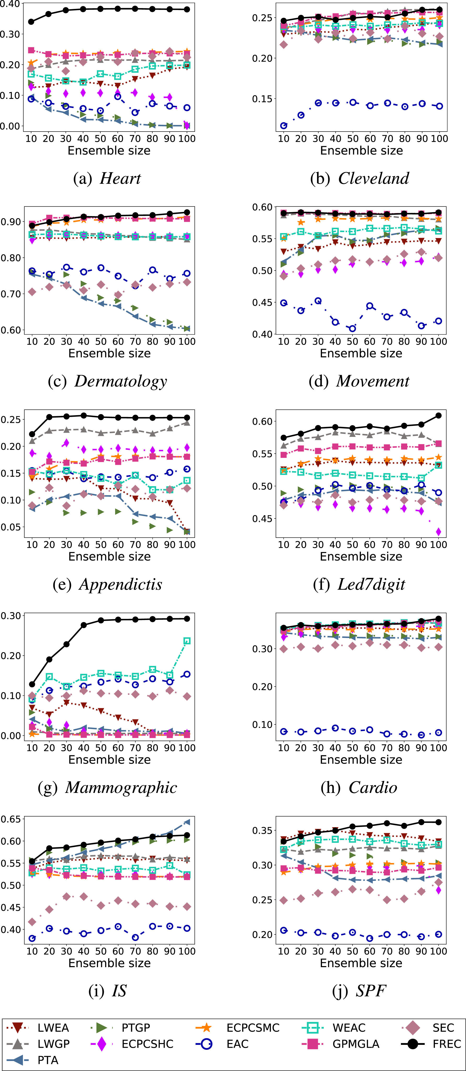
HS results with the ensemble size.

Ten state-of-the-art ensemble clustering algorithms, namely, locally weighted evidence accumulation (LWEA) [14], locally weighted graph partitioning (LWGP) [14], probability trajectory accumulation (PTA) [16], probability trajectory based graph partitioning (PTGP) [16], ensemble clustering by propagating cluster-wise similarities with hierarchical consensus function (ECPCS-HC) [18], ensemble clustering by propagating cluster-wise similarities with meta-cluster-based consensus function (ECPCS-MC) [18], evidence accumulation clustering (EAC) [5], weighted evidence accumulation clustering (WEAC) [15], graph partitioning with multi-granularity link analysis (GPMGLA) [15], and spectral ensemble clustering (SEC) [26] are selected to compare the ensemble performance of FREC. Moreover, two other non-ensemble state-of-the-art clustering methods, deep temporal clustering representation (DTCR) [37] and robust temporal feature network (RTFN) [50] are also used to compare the performance of the newly proposed method. For FREC, Łukasiewicz t-norm and Equation (9) are used to calculate the fuzzy similarity. As for other compared algorithms, there is no extra parameter for EAC, and the specific parameters of the remaining methods are set according to the recommendations or optimal values given in the corresponding papers. More specifically, the core settings are listed as follows.

LWEA, LWGP: θ = 0.4;

PTA, PTGP: $K=\sqrt{N}/2$ , $T=\sqrt{N}/2$ where N indicates the number of the graph nodes;

ECPCSHC, ECPCSMC: t = 20;

WEAC, GPMGLA: α = 0.5, β = 2;

SEC: μ = 1;

DTCR: m₁ = 100, m₂ = 50, m₃ = 50, λ = 1e - 1, lr = 1e - 4;

RTFN: CNNchannel = 128, kernelsize = 11, l _rate  (0) =0.01, d _rate  = 0.1.

Fig. 8

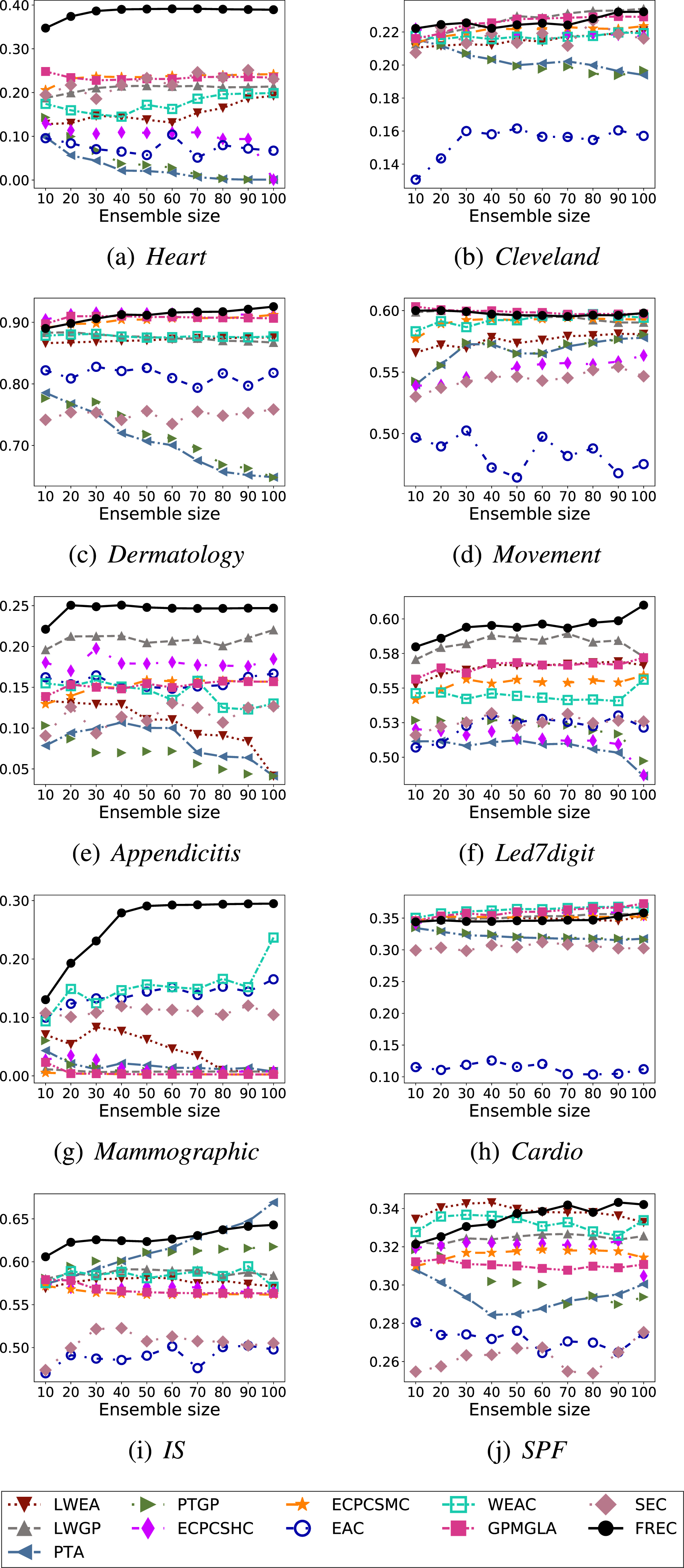
NMI results with the increased ensemble size.

Fig. 9

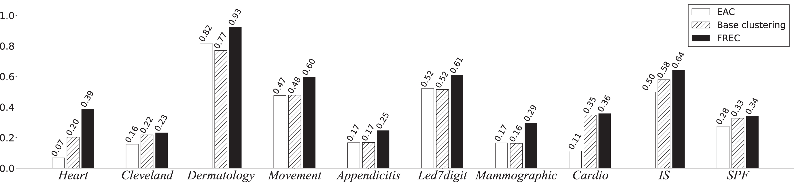
NMI results of FREC versus the parallel EAC and base clustering.

4.2 The influence of ensemble size

Figures 7 8 show the experimental results for different ensemble sizes, including two indexes of HS and NMI on ten benchmark datasets. The various contrastive algorithms use different colours, lines and markers, as the legend details. Apparently, for the proposed FREC, as the ensemble size increases, the results on nearly all datasets deliver an upward trend regardless of the evaluation criteria, which is in line with the objective of ensemble methods. More specifically, considering HS, FREC shows significantly superior performance on datasets Heart, Appendictis, Led7digit and Mammographic, i.e. no matter how large the ensemble size is, FREC can invariably outperform the other ten ensemble techniques. For Dermatology and SPF, if the ensemble size is less than 40, the effect of FREC is slightly lower than that of GPMGLA and LWEA, respectively, but exceeds that of the other nine methods. If the ensemble size is more significant than 40, the proposed method performs superiorly, outperforming all different ways. While Cleveland, Cardio, and IS are not optimal in all ensemble sizes, FREC can always exceed most comparison approaches and always shows the best or second best performance if the ensemble size is maximum. Finally, for Movement, as the ensemble size increases, the performance of FREC tends to stabilise rapidly, and there is no apparent transformation trend. However, it can still surpass almost all contrastive algorithms.

While using the evaluation index NMI, the results are resemblance. For Heart, Appendictis, Led7digit and Mammographic, FREC can accomplish best values at any ensemble size, and the performance grows and stabilises as the ensemble size boosts. Regarding Cardio, although FREC is slightly lower than some methods if the ensemble size is less than 90, FREC still performs satisfactorily if the ensemble size is the largest, which ranks third. The curves of FREC may be slightly lower for the remaining datasets than individual algorithms at a particular ensemble size. Still, FREC can consistently achieve better results, especially at the largest ensemble size.

4.3 Comparison to the parallel EAC and base clustering

The algorithm EAC, which means the original co-association based ensemble scheme that does not consider cluster reliability, always conducts poorly in both HS and NMI. As exampled in Fig. 7(b), 7(d), 7(h) and 7(iFor the three clusters), EAC conveys the worst effect regardless of the ensemble size by comparing the other ten ensemble algorithms. To more comprehensively recognise the effect of using the cluster reliability induced by fuzzy-rough set, this part compares FREC and the parallel EAC in detail in the form of a histogram.

Since all ensemble strategies primarily achieve more satisfactory results at larger ensemble sizes, FREC and EAC use the pool containing 100 base clusterings. Moreover, both algorithms are run 100 times to acquire the average results. In addition, the algorithms in the base clustering pool (k-means) are also averaged to compare the ensemble performance.

Table 5

HS results of FREC versus other ensemble algorithms

Dataset	Heart		Cleveland		Dermatology		Movement		Appendicitis
Algorithm	Ave	Best	Ave	Best	Ave	Best	Ave	Best	Ave	Best
LWEA	0.192 v	0.192	0.244 v	0.244	0.858 v	0.858	0.546 v	0.546	0.041 v	0.041
LWGP	0.214 v	0.214	0.260 v	0.260	0.851 v	0.851	0.580 v	0.594	0.244 v	0.245
PTA	0.001 v	0.001	0.217 v	0.217	0.603 v	0.603	0.564 v	0.564	0.041 v	0.041
PTGP	0.001 v	0.001	0.220 v	0.220	0.603 v	0.603	0.567 v	0.573	0.041 v	0.041
ECPCSHC	0.001 v	0.001	0.241 v	0.241	0.859 v	0.859	0.521 v	0.521	0.198 v	0.198
ECPCSMC	0.243 v	0.243	0.250 v	0.250	0.912 v	0.912	0.581 v	0.584	0.180 v	0.180
WEAC	0.198 v	0.198	0.243 v	0.243	0.858 v	0.858	0.562 v	0.562	0.136 v	0.136
GPMGLA	0.235 v	0.235	0.256 v	0.256	0.907 v	0.907	0.590 v	0.590	0.180 v	0.180
SEC	0.224 v	0.380	0.227 v	0.227	0.732 v	0.923	0.520 v	0.584	0.122 v	0.154
DTCR	0.288 v	0.288	0.250 v	0.260	0.851 v	0.851	0.460 v	0.460	0.298 *	0.298
RTFN	0.375 v	0.375	0.270 *	0.270	0.880 v	0.923	0.558 v	0.558	0.248 v	0.248
FREC	0.380	0.380	0.261	0.261	0.926	0.926	0.591	0.591	0.253	0.253
Summary	(11/0/0)		(10/0/1)		(11/0/0)		(11/0/0)		(10/0/1)
Dataset	Led7digit		Mammographic		Cardio		IS		SPF
Algorithm	Ave	Best	Ave	Best	Ave	Best	Ave	Best	Ave	Best
LWEA	0.532 v	0.532	0.005 v	0.005	0.363 v	0.363	0.556 v	0.556	0.334 v	0.334
LWGP	0.565 v	0.566	0.005 v	0.005	0.368 v	0.382	0.560 v	0.610	0.328 v	0.357
PTA	0.474 v	0.474	0.005 v	0.005	0.330 v	0.330	0.643 *	0.643	0.285 v	0.285
PTGP	0.477 v	0.507	0.005 v	0.005	0.332 v	0.363	0.603 v	0.633	0.303 v	0.341
ECPCSHC	0.429 v	0.429	0.005 v	0.005	0.357 v	0.357	0.521 v	0.521	0.264 v	0.264
ECPCSMC	0.544 v	0.545	0.001 v	0.001	0.352 v	0.356	0.519 v	0.519	0.301 v	0.301
WEAC	0.532 v	0.532	0.237 v	0.237	0.368 v	0.368	0.524 v	0.524	0.330 v	0.330
GPMGLA	0.566 v	0.566	0.001 v	0.001	0.375 v	0.375	0.519 v	0.519	0.296 v	0.296
SEC	0.477 v	0.554	0.098 v	0.289	0.304 v	0.364	0.452 v	0.629	0.275 v	0.376
DTCR	0.500 v	0.500	0.300 *	0.300	0.330 v	0.330	0.535 v	0.535	0.260 v	0.260
RTFN	0.575 v	0.575	0.290 v	0.290	0.380 *	0.380	0.593 v	0.593	0.351 v	0.351
FREC	0.609	0.609	0.292	0.292	0.379	0.380	0.613	0.613	0.362	0.380
Summary	(11/0/0)		(10/0/1)		(10/0/1)		(10/0/1)		(11/0/0)

Table 6

NMI results of FREC versus other ensemble algorithms

Dataset	Heart		Cleveland		Dermatology		Movement		Appendicitis
Algorithm	Ave	Best	Ave	Best	Ave	Best	Ave	Best	Ave	Best
LWEA	0.192 v	0.192	0.221 v	0.221	0.875 v	0.875	0.581 v	0.581	0.041 v	0.041
LWGP	0.214 v	0.214	0.232 v	0.232	0.867 v	0.867	0.590 v	0.611	0.220 v	0.221
PTA	0.001 v	0.001	0.194 v	0.194	0.648 v	0.648	0.578 v	0.578	0.041 v	0.041
PTGP	0.001 v	0.001	0.197 v	0.197	0.648 v	0.648	0.581 v	0.589	0.041 v	0.041
ECPCSHC	0.001 v	0.001	0.217 v	0.217	0.912 v	0.912	0.564 v	0.564	0.185 v	0.185
ECPCSMC	0.242 v	0.242	0.224 v	0.224	0.912 v	0.912	0.593 v	0.594	0.157 v	0.157
WEAC	0.199 v	0.199	0.219 v	0.219	0.877 v	0.877	0.594 v	0.594	0.130 v	0.130
GPMGLA	0.234 v	0.234	0.229 v	0.229	0.906 v	0.906	0.597 v	0.597	0.157 v	0.157
SEC	0.231 v	0.389	0.216 v	0.295	0.758 v	0.923	0.547 v	0.606	0.127 v	0.369
DTCR	0.287 v	0.287	0.227 v	0.231	0.905 v	0.905	0.460 v	0.460	0.294 *	0.294
RTFN	0.382 v	0.382	0.245 *	0.245	0.869 v	0.923	0.584 v	0.584	0.241 v	0.241
FREC	0.389	0.389	0.234	0.234	0.925	0.925	0.598	0.598	0.247	0.247
Summary	(11/0/0)		(10/0/1)		(11/0/0)		(11/0/0)		(10/0/1)
Dataset	Led7digit		Mammographic		Cardio		IS		SPF
Algorithm	Ave	Best	Ave	Best	Ave	Best	Ave	Best	Ave	Best
LWEA	0.567 v	0.567	0.007 v	0.007	0.353 v	0.353	0.571 v	0.571	0.333 v	0.333
LWGP	0.573 v	0.577	0.007 v	0.007	0.357	0.369	0.584 v	0.617	0.326 v	0.349
PTA	0.486 v	0.486	0.007 v	0.007	0.318 v	0.318	0.669 *	0.669	0.300 v	0.300
PTGP	0.497 v	0.524	0.007 v	0.007	0.316 v	0.343	0.618 v	0.650	0.294 v	0.336
ECPCSHC	0.487 v	0.487	0.007 v	0.007	0.355 v	0.355	0.566 v	0.566	0.305 v	0.305
ECPCSMC	0.559 v	0.560	0.002 v	0.002	0.353 v	0.356	0.562 v	0.562	0.314 v	0.314
WEAC	0.556 v	0.556	0.237 v	0.237	0.366 *	0.366	0.571 v	0.571	0.334 v	0.334
GPMGLA	0.572 v	0.572	0.002 v	0.002	0.373 *	0.373	0.563 v	0.563	0.311 v	0.311
SEC	0.526 v	0.585	0.104 v	0.292	0.303 v	0.354	0.505 v	0.660	0.275 v	0.363
DTCR	0.480 v	0.480	0.300 *	0.300	0.310 v	0.310	0.555 v	0.555	0.210 v	0.210
RTFN	0.584 v	0.585	0.292 v	0.292	0.361 *	0.361	0.575 v	0.575	0.339 v	0.339
FREC	0.610	0.610	0.295	0.295	0.358	0.359	0.643	0.643	0.342	0.361
Summary	(11/0/0)		(10/0/1)		(7/1/3)		(10/0/1)		(11/0/0)

Without overloading similar results, the NMI is used to report the experiment evaluation. As shown in Fig. 9, FREC consistently achieves a better clustering effect relative to the parallel EAC and base clustering on all datasets. Especially for Heart, Dermatology, Movement and Mammographic, FREC reports the best clustering results while achieving a satisfactory improvement, illustrating the advantage which considers the cluster reliability and the superiority of FREC.

4.4 Comparison to other clustering algorithms

In order to comprehensively evaluate the performance of the proposed algorithm, experimental comparisons are carried out against the other eleven state-of-the-art methods. The results are summarised in Tables 5 6. Note that the results of EAC have been analysed in Section 4.3 and will not be repeated in this part.

Recall reported results, ensemble algorithms always work best using more ensemble size. Thus, all comparison ensemble methods employ the results with an ensemble size of 100, and the average and best results for each dataset are shown in columns Ave and Best, respectively. To describe the experimental results more obviously, the best results are highlighted in bold. Moreover, the second best results are highlighted with an underline to make the information in the table easier to follow.

Considering the metric HS, FREC achieves optimal average performance relative to the other eleven algorithms in most datasets, including Heart, Dermatology, Movement, Leg7digit and SPF. As for the results in column Best, although a bit inferior to one or two approaches occasionally, FREC is the best or second best in most cases. For the remaining datasets, the average performance of FREC is slightly lower than individual algorithms. Still, FREC shows a satisfactory clustering effect compared with the other techniques.

Now, take an observation of the evaluation NMI, the clustering result is highly analogous to HS. For datasets Heart, Cleveland, Dermatology, Movement, Appendicitis, Leg7digit, Mammographic and SPF, the proposed method can consistently surpass most contrasting approaches. For dataset IS, consistent with the HS, FREC is slightly inferior to PTA, ranking second in all ensemble methods. The main difference from HS is the dataset Cardio. FREC is slightly lower than WEAC and GPMLGA by 0.008 and 0.015, respectively. Nevertheless, compared with the remaining algorithms, FREC still shows excellent performance.

In general, the average and best results of FREC are equal in most cases, which means that the FREC is relatively stable and the results are less serendipitous. At the same time, regardless of the average or best results, FREC always achieves the most significant or second best effect, which illustrates the rationality of the research in this paper.

4.5 Statistical analysis

Paired t-test is used throughout the present experimental studies to show any statistically significant differences between different approaches. This helps ensure that the results are not obtained by chance. The t-test results are summarised at the end of each table, counting the number of statistically better(v), equivalent(space) or worse(*) cases for FREC in comparison to each algorithm. In all experiments reported, the threshold of significance is set to 0.05. For example, in Table 6, (11/0/0) in the column Heart indicates that the clustering performance returned by FREC performs better than other ensemble methods in eleven cases, equivalently well in no case, and worse than other approaches in no case. It can be clearly seen that whether the evaluation index is HS or NMI, the statistical results of FREC are better than other methods in most cases, especially for the HS indicator, FREC can surpass all other algorithms on more than half of the datasets. Statistical analysis experiments show that in 100 repeated experiments, the overall performance of FREC is relatively stable, which is better than most algorithms.

4.6 Time complexity analysis

As shown in Algorithm 4, the computing cost of the proposed FREC mainly includes three parts: (1) For UDC, this function mainly consists of three loops with a time complexity of O (mk (k - 1)). In particular, each instance needs to traverse to find the lower approximation when calculating UD in the inner loop, and this process will consume O (n²); (2) As for CMC, this part mainly calculates the upper triangular matrix of $\tilde{A}$ , and the time complexity is O (n²k); (3) Finally, CSC computes the eigenvectors of adjacency matrix and performs fast clustering, with a time complexity of O (ndk). Thus, the total cost of FREC is O (mk (k - 1) + n² + ndk).

Table 7

Time complexity comparison of different algorithms (seconds)

Dataset	LWEA	LWGP	PTA	PTGP	ECPCSHC	ECPCSMC	WEAC	GPMGLA	SEC	DTCR	RTFN	FREC
Heart	0.01	0.12	0.02	0.06	0.18	0.21	0.01	1.65	0.01	36.36	1.34	18.76
Cleveland	0.01	0.18	0.02	0.05	0.22	0.25	0.01	2.54	0.01	38.52	1.47	19.50
Dermatology	0.01	0.11	0.01	0.06	0.24	0.31	0.01	3.47	0.01	227.09	1.49	19.59
Movement	0.01	0.11	0.02	0.06	0.20	0.23	0.01	2.43	0.01	437.69	1.63	22.41
Appendicitis	0.01	0.12	0.01	0.05	0.05	0.06	0.01	0.36	0.01	15.51	0.18	4.34
Led7digit	0.01	0.13	0.01	0.05	0.37	0.35	0.06	4.81	0.01	28.61	2.64	36.49
Mammographic	0.01	0.31	0.01	0.04	0.76	0.72	0.16	12.80	0.01	38.08	2.81	76.43
Cardio	0.01	0.54	0.01	0.10	3.37	2.57	1.45	55.96	0.01	368.16	4.52	404.51
IS	0.01	0.56	0.01	0.06	3.84	3.27	1.60	72.76	0.01	352.29	4.48	398.55
SPF	0.01	0.39	0.01	0.06	2.76	2.21	1.13	52.29	0.01	428.80	4.36	407.69

To compare the running time gap with other methods, the running time (seconds) of each algorithm is reported in Table 7. The experimental CPU used is i7-12700, and the memory is 24G. It can be seen that after considering the data features, the running time of FREC is significantly higher than that of other comparison methods. Especially as the number of instances continues to increase, the time of FREC increases significantly. In comparison, methods such as LWEA, SEC, and RTFN have achieved better running time. The above implementation shows that the time efficiency of FREC is relatively poor, which requires further optimisation in subsequent work.

5 Conclusion

This paper explores the role of considering cluster reliability using fuzzy-rough set in co-occurrence based ensemble clustering, and guides a fuzzy-rough ensemble approach. The experimental results indicate that the reliability induced by fuzzy-rough lower approximation is effective and can be reasonably employed in the task of ensemble clustering. Compared with other ensemble algorithms that ignore attributes and only employ base clustering results, FREC demonstrates the advantage of viewing feature information. Meanwhile, compared with the parallel version and base clustering, FREC shows its superiority again.

Nonetheless, from the time experiment, the efficiency of FREC is relatively slow. This is mainly due to the high time complexity of the algorithm. For large sample datasets, it will take a lot of time to calculate the lower approximation for each object. In future work, the idea of KD-tree [44] can be introduced to improve the running speed of the algorithm further. In addition, in Equation (23), if the two instances do not belong to the same cluster, it may not be a better choice to assign the adjacency matrix to 0 directly. Further mining the implicit connection between instances of different clusters helps improve the clustering performance.

Whilst promising, further work remains. The performance of the ensemble strategy and multi-density cluster designs is worth further exploration. In addition, the implied relationship of the objects in the same base clustering but the different clusters is a valuable route of investigation. Moreover, a more comprehensive comparison of ensemble methods over diverse datasets from the real-world domains, such as mammographic risk assessment [46, 47] would construct the foundation for a broader series of issues for future research.