An optimized fuzzy based FP-growth algorithm for mining temporal data

Abstract

Data mining is one of the emerging technologies used in many applications such as Market analysis and Machine learning. Temporal data mining is used to get a clear knowledge about current trend and to predict the upcoming future. The rudimentary challenge in introducing a data mining procedure is, processing time and memory consumption are highly increasing while trying to improve the accuracy, precision or recall. As well as, while trying to reduce the processing time or memory consumption, accuracy, precision and recall values are reducing significantly. So, for improving the performance of the system and to preserve the memory and processing time, Three-Dimensional Fuzzy FP-Tree (TDFFPT) is proposed for Temporal data mining. Three functional modules namely, Three-Dimensional Temporal data FP-Tree (TTDFPT), Fuzzy Logic based Temporal Data Tree Analyzer (FTDTA) and Temporal Data Frequent Itemset Miner (TDFIM) are integrated in the proposed method. This algorithm scans the database and generates frequent patterns as per the business need. Every time a client purchases a new item, it gets stored in the recent database layer instead of rescanning the entire records which are placed in the old layer. The results obtained shows that the performance of the proposed model is more efficient than that of the existing algorithm in terms of overall accuracy, processing time, reduction in the memory utilization, and the number of databases scans. In addition, the proposed model also provides improved decision making and accurate pattern prediction in the time series data.

1 Introduction

Data mining is one of the most essential processes which is used in multiple domains such as Bioinformatics, Customer segmentation, Customer relationship and Management, Future healthcare, Intrusion Detection, Market Basket Analysis, Manufacturing Engineering and Resource provision planning [1]. Recent advancements in data mining are used to predict some disease occurrence probability by analyzing the hereditary data and gene sequences. Apart from handling databases, data mining procedures are used to create knowledgebases which are inevitable in the field of Artificial Intelligence and Machine Learning. The applications of data mining procedures are omnipresent in this data driven commercial world at present.

Temporal databases contain the time of the event occurrence along with the event information. Modernizations in data handling increase the volume of the temporal databases. Even a simple selfie photograph contains the timestamps and geotags. This huge volume of temporal database is more useful than normal databases by providing the timestamp instances. At the same time the complexity of temporal data mining is also higher than the conventional database handling due to the discrete, continuous, constant stepwise, period based or hybrid time logging nature [2, 3]. The prediction curves are calculated more accurately while using temporal databases instead of normal databases. The precision in trend analysis is also higher in case of temporal databases.

Different types of temporal databases such as Uni-temporal, Bi-Temporal and Tri-Temporal are requiring more efficient algorithms to extract the useful information and knowledge from them [4]. The temporal databases are hugely diversified due to multiple time represent formats. The time representation format varies from simple YYYY-MMM-DD format to thoroughgoing DD-MM-YYYY::HH:MM:SS format. A temporal data mining technique should have a smooth interface to handle different time representation formats. Though conventional data mining procedures can handle the temporal databases by discarding the time-data, they lack the ability to define the validity of the record over the information decay gradient and to cover entity types, temporal relationship types and temporal attributes [5]. There are several basic data mining algorithms such as Apriori, FP-Tree, K-Means, k-nearest neighbor (kNN), Support Vector Machines (SVM), Page Rank (PR), Expectation-Maximization (EM), Naïve Bayes (NB) and Classification & Regression Tree (CART) are available with their own advantages and limitations. FP-Tree is selected as the base in this work to handle the temporal data due to its simplicity, lesser number of input scanning than the other methods and the minimum computational complexity O (n).

2 Existing methods

A detailed literature review is performed in the topic of Temporal Data mining and some of the reputed works are taken here for elaborate analysis to understand the challenges, concepts and resolutions. The exacted procedures are A New Methodology for Mining Frequent Itemsets on Temporal Data [6], Learning from heterogeneous temporal data in electronic health records [7], Hierarchical evolving Dirichlet processes for modeling nonlinear evolutionary traces in temporal data [8] and Burst Topic Detection in Real Time Spatial-Temporal Data Stream [9]. The performance of all these methods are analyzed in terms of Accuracy, Precision, Recall, F-Score, Processing time and Memory consumption.

2.1 A New Methodology for Mining Frequent Itemsets on Temporal data (MMFIT)

Frequent itemset mining with time cubes concept is introduced in MMFIT work. The time cubes are introduced over the existing Apriori algorithm to restrict the time intervals of the temporal data for performance enhancements. MMFIT can track the frequent patterns that occurs or change periodically. These frequent patterns are identified by a new density threshold of MMFIT. The new density threshold is also used to address the overestimating problem of time periods in temporal data. The initial Time Cubes are represented as Basic Time Cubes (BTC) and Different algorithms such as mining frequent itemsets using time cubes, mining large itemsets and candidate generation are introduced in MMFIT. The purpose of introducing time cubes is to improve the processing speed which is working as declared in MMFIT. Some suboptimal BTCs cause a reduction in accuracy and prediction which is the limitation of MMFIT.

2.2 Learning from heterogeneous temporal data in electronic health records (LHTDE)

LHTDE is included here due to its ability to handle large volume of heterogeneous electronic health records. Time series based piecewise aggregation approximation, Symbolic aggregate approximation and Sequence patterns are discussed in this work. Sequence generation, sequence clustering, random subsequence selection and random dynamic subsequence methods are used in LHTDE work. The generalized heterogeneous processing nature of this work makes it possible to use LHTDE with any temporal dataset. The performance of this work is measured using large volume of longitudinal timestamped clinical data. High processing speed is the main advantage of LHTDE as authors stated. Accuracy and precision are affected while using noisy data –which is the limitation of this work.

2.3 Hierarchical evolving Dirichlet processes for modeling nonlinear evolutionary traces in temporal data (HEDP)

HEDP is introduced to automate the process of content organization in temporal text data. Number of clusters, Cluster parameters and cluster distribution properties of a typical temporal text data are analyzed clearly in this work. Challenges such as uncertain number of branches and branch cluster parameter evolutions are well handled in HEDP work. The infinite dimension generalization of distribution over distributions ensures the accuracy of this method. Different methods are used in HEDP for Multivariate Gaussian distribution and Discrete data with multinomial distribution. The introduction of Hierarchical Dirichlet Processes increases the accuracy and it also increases the computational complexity to O (log(N _t ) N _t ). The increased computational complexity reflects on the processing speed tangibly. Higher processing time is observed as the limitation of HEDP.

2.4 Burst Topic Detection in Real Time Spatial-Temporal Data Stream (BTDRTS)

The purpose of BTDRTS introduction is the detect the burst term or topic detection in noisy and diluted social media information. The challenges of detecting burst topic from social media data are the decentralized sparse of data, highly noisy erratic nature of data, variation in distribution frequency and the need for real time topic tracking. These challenges are well addressed in the BTDRTS work. BTDRTS has three functional blocks, they are, Fast detection method for burst topic, data prediction for hiding burst term detection in data stream and a dedicated Spatial Temporal topic detection model. BTDRTS work provides assorted procedures for Evolving curve fitting, Data prediction, Temporal characteristics calculation and Burst term judgement. The processing speed of BTDRTS meets out the requirement for real time processing which is the main advantage of this method. The domain specific approach causes a decrease in accuracy and prediction while using diversified heterogeneous datasets –which is the limitation of this work.

3 Motivation to proposed work

Proposed TDFFPT is designed based on the fundamental principles of FP-Growth. Empathizing the basic concepts of Frequent Pattern Tree (FP-Tree) and FP-Growth are required here to explain the proposed method intricately.

3.1 FP-Tree

FP-Tree is a compact data structure used to store a dataset and transactions. The complete details of a transaction table can be represented by the FP-Tree [10, 11]. That is each element and their related elements in a transaction can be directly mapped to a FP-Tree. Different transactions with similar itemsets are stored in a compact way by sharing the same overlapped structure in the FP-Tree. The construction of FP-Tree is performed by a simple Algorithm 1.

Algorithm 1: FP-Tree Construction

Input: Transaction Table

Output: FP-Tree

Step 1: Scan the dataset to determine support count of each item

Step 2: Sort the frequent items in descending order

Step 3: Scan the dataset transaction by transaction to construct the Tree

3.1 Creating a new branch for unique transactions and assign, initial counter value = 1 for each item

3.2 Share the tree structure for common prefix itemsets and increment the counter for each item

Step 4: Repeat step 3 until all transactions have been mapped to the FP-Tree

3.2 FP-growth

FP-Growth is a frequent itemset mining procedure which uses the FP-Tree representation of transaction table. FP-Growth is well known for it’s efficient frequent itemset mining from the compact FP-Tree representations [12, 13]. The divide and conquer approach followed by the FP-Growth engenders this efficient frequent itemset mining operation swiftly.

Algorithm 2: FP-Growth

Input: FP-Tree

Output: Frequent patterns

Step 1: Create prefix paths for suffix node –all paths that ends with the suffix node are to be included

Step 2: Add the support counts of entangled nodes using prefix path tree

2.1 If the sum of supports > minsup (minimum support count), then the suffix comes under the frequent category

2.2 If the sum is inferior to the minsup, then the suffix is discarded from further analysis

Step 3: Construct the Conditional FP-Tree by converting the prefix paths

• 3.1 Modify the support counts all over the prefix paths based on the actual number of transactions carrying the particular itemset.

• 3.2 Discard the nodes of the selected suffix and truncate the prefix paths

• 3.3 Eliminate the infrequent items

• Repeat from Step 3.1 to 3.3 for all prefix paths of chosen suffix

Step 4: Repeat from Step 1 to 3 for all suffix nodes

Proposed system model

A Three-dimensional Fuzzy FP-Tree for Temporal Data Mining (TDFFPT)

The proposed method TDFFPT is the integration of three functional blocks. They are, the Three-Dimensional Temporal Data FP-Tree, Fuzzy Logic based Temporal Data Tree Analyzer and Temporal Data Frequent Itemset Miner.

4.1 Three-dimensional Temporal Data FP-Tree (TTDFPT)

Temporal data are collected dynamically in case of Retail applications. There are no fixed time durations involved in retail data acquisition [14]. Therefore, the records are added dynamically during the billing process. The retail temporal dataset can be divided into 4 weeks for monthly analysis or 52 weeks for yearly analysis to construct a TTDFPT. This weekly separation approach provides many frequent patterns for weekdays and weekends. The TTDFPT construction is explained here with an example temporal dataset transaction table given as Table 2.

Table 2

Example transaction table

TID	Timestamp	Items	Sorted
1	01-01-2019::06 : 45 : 42	{a,b,c}	{a,c,b}
2	01-01-2019::08 : 02 : 29	{a,d,e}	{e,a,d}
3	02-01-2019::10 : 12 : 30	{a,b,e}	{e,a,b}
4	02-01-2019::16 : 04 : 45	{b,c,d,e}	{e,c,d,b}
5	03-01-2019::10 : 15 : 52	{a,c,d,e}	{e,a,c,d}
6	04-01-2019::12 : 33 : 34	{d,e}	{e,d}
7	04-01-2019::17 : 05 : 53	{c,e}	{e,c}
8	05-01-2019::11 : 45 : 07	{a,d}	{a,d}
9	06-01-2019::09 : 58 : 20	{b,c,e}	{e,c,b}
10	07-01-2019::16 : 22 : 19	{a,c,e}	{e,a,c}

The normal FP-Tree constructed for the above transaction table is given in Fig. 1.

Fig. 1

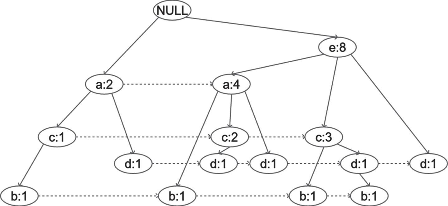
Example FP-Tree.

The frequencies of each item involved in the transactions are calculated and given in Table 3.

Table 3

Frequencies of items

Item	Frequency
e	8
a	6
c	6
d	5
b	4

The FP-Tree is constructed by the standard procedure given in algorithm 1. Similarly, the successive 3 weeks transactions are constructed as FP-Trees for one-month analysis. TTDFPT takes place where there are similar purchasing pattern repeats in different weeks all over the month

4.2 Fuzzy Logic based Temporal Data Tree Analyzer (FTDTA)

FTDTA is used to provide the utility mining determination-based bias for waning and waxing nodes based on the transition curves. The incorporation of High Utility Itemset Mining [15, 16] over Frequent Itemset Mining enables the FTDTA to preserve the weights of rare items –brought to the next functional block in which detection of rare patterns is possible. The high utility biased weights cut downs the elimination of rare but profitable items from entering into waning node category.

The Symbols and their meanings which are used in this section are given in Table 4.

Table 4

Symbols and meanings

Symbols	Meaning
T	Transaction Table Set
{t1, t2⋯ t n  }	Transaction elements in which ∀i = 1 → n : t i  ∈ T
I t x	Itemset of a Transaction t x
{i1, i2, ⋯ i m  }	Item elements
Δ ={ δ1, δ2 … δ|ξ| }	Temporal entity set in which each δ x  ∈ Δ where ξ > 0
U ={ u1, u2 … u|ξ| }	Utility set of Δ
τ min	Minimum Utility Threshold
s min	Minimum Support
c min	Minimum Confidence
u o  (i p , t q )	Transaction Utility of t q for Item i P
s (i q )	External Utility of Item i q
f (o, s min )	Utility function of u o with s min
$u_0^c$	Cyclic Utility of u o
Ω ={ ω(i1,t1), ω(i2,t1), … ω(i1,t2), … ω(i m ,t n ) }	Weight index Set where ω(i x ,t y ) is the weight element
for item i x in Transaction t y

The first phase of FTDTA begins with the construction of a Utility Table (Γ) as a Triple Γ = I, U, Δ. The external utility for item i _x is calculated as s (i _x ) = U (i _x ). The utility of an item i _x in transaction t _y is calculated f (o (i _x , t _x ) , s (i _x )). The weight index ω_{(i x ,t y )} is calculated by using the following equation

$\omega \left({\mathrm{i}}_{\mathrm{x}},{\mathrm{t}}_{\mathrm{y}}\right);=\sum _{\mathrm{x}=1}^{\mathrm{m}}*\sum _{\mathrm{x}=1}^{\mathrm{m}}*\sum _{\mathrm{z}=1}^{\xi }\frac{\left(\xi \times \eta \left({\mathrm{i}}_{\mathrm{x}}\in {\mathrm{I}}_{{\mathrm{t}}_{\mathrm{y}}}\right)\right)}{{\delta }_{\mathrm{z}}}$(1)

Where ξ = 4 for weekly analysis of a month data, η is the number of instances of item i _x in transaction t _y

The temporal utility support (TUS (i _x )) of item i _x is calculated as

$\mathit{TUS}\left(i_x\right)=\frac{\sum _{x=1}^n\sum _{y=1}^m\eta \left(i_x\in I_{t_y}\right)}{m\times n}$(2)

The temporal utility confidence TUC (i _x  →  i _y ) of Item i _x over i _y is calculated as

$\mathit{TUC}\left(i_x\to i_y\right)=\frac{\mathit{TUS}\left(i_x\right)\cup \mathit{TUS}\left(i_y\right)}{\mathit{TUS}\left(i_x\right)}$(3)

The fuzzy weight bias for item i _x of transaction t _y for the temporal entity δ _z is calculated as

$\mu \left(i_x,t_y,{\delta }_z\right)=\frac{\sum _{z=1}^{\xi }{\omega }_{\left(i_x,t_y\right)}}{\xi }$(4)

The normalization process is performed by using the Equation (5) –given below

${\mu }_N\left(i_x,t_y,{\delta }_z\right)=\frac{{\mathrm{e}}^{\mu \left(i_x,t_y,{\delta }_z\right)}}{\sum _{z=1}^{\xi }\left({\mathrm{e}}^{\mu \left(i_x,t_y,{\delta }_z\right)}\right)}$(5)

Then the Priority index LOW, MEDIUM or HIGH for waning and waxing nodes are assigned based on the following condition

$\begin{array}{cc}\hfill & \mathrm{Computation\; of\; waning\; and\; waxing\; nodes}\hfill \\ \hfill & =\{\begin{array}{c}\hfill \mathit{waxing\; node\; if}{\omega }_n>{\omega }_{n-1}\hfill \\ \hfill \mathit{waning}\mathit{node}\mathit{if}{\omega }_n<{\omega }_{n-1}\hfill \\ \hfill \mathit{normal}\mathit{otherwise}\hfill \end{array}\hfill \end{array}$(6)

4.3 Temporal Data Frequent Itemset Miner (TDFIM)

TDFIM gets the input from FTDTA, by which it performs Mining Frequent Closed Itemsets, handling incremental datasets, handling if uncertain data, mining high utility itemsets, finding sequential patterns and detecting rare patterns. It follows the conventional FT-Growth procedure to find frequent patterns of each layer TTDFPT. A virtual layer with the means of 4 layers are calculated and maintained in memory to trace the frequent temporal patterns as given in the following algorithm and typical TTDFPT is illustrated in Fig. 2.

Fig. 2

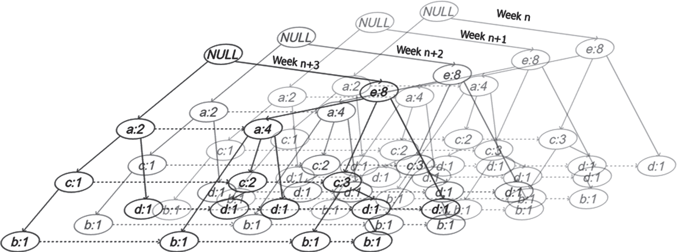
Illustration for typical TTDFPT.

Fig. 2.1

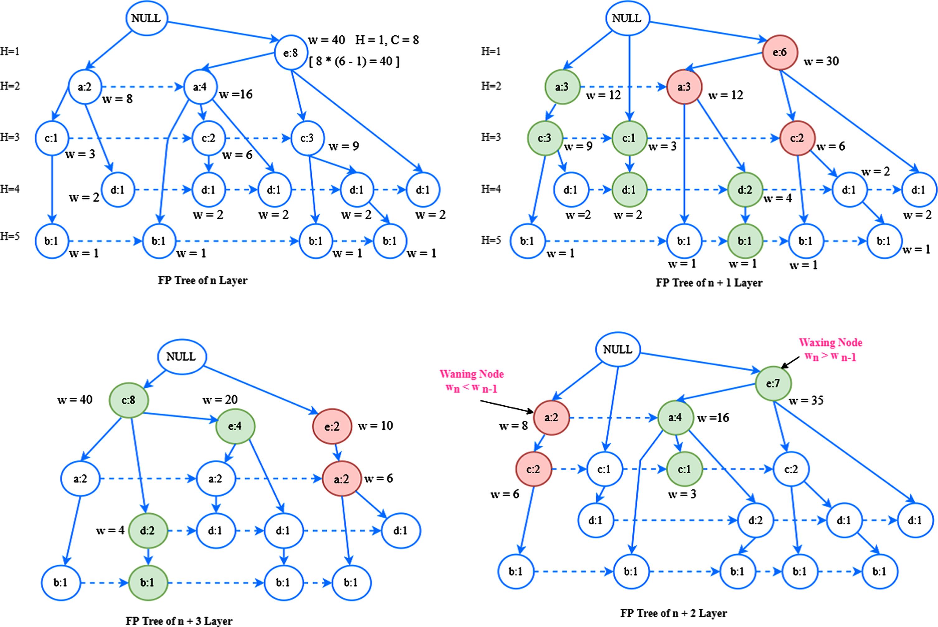
Computation of waxing and waning node.

There are multiple changes to get new items added in the successive months where some existing items will not get entry. These conditions are handled in TTDFPT by introducing the waning nodes and waxing nodes. TTDFPT holds only 4 layers of FP-Tree in memory. Whenever a new layer is added, the earlier layer is discarded from TTDFPT. Therefore, at any time there are only FP-Tree layers are maintained in TTDFPT to preserve memory and processing time. Waning nodes represent the disappearing items and waxing nodes represent emerging items over the continuance. The waning and waxing rate in TTDFPT is altered based on the bias provided by the Fuzzy logic based temporal data tree analyzer which is shown in above Fig. 2.1.

Algorithm 3: TDFIM

Input: TTDFPT tree with FTDTA data

Output: Frequent, sequential and rare temporal patterns

Step 1: Create a set of Prefix paths for suffix nodes in all layers of TTDFPT as,

ρ ={ ρ₁ = { ρ₁₁, ρ₁₂, … ρ_1n } , ρ₂ = { ρ₂₁, ρ₂₂, …     ρ_2n } , … ρ _ξ  = { ρ_ξ1, ρ_ξ2, … ρ _ξn  }}

Step 2: Construct the conditional FP-Trees for ρ₁ to ρ _ξ by steps 2,3,4 of algorithm 2.

Step 3: Construct the virtual temporal tree layer as $\frac{1}{\xi }\times {\sum }_{\mathrm{i}=1}^{\xi }\rho \circ \left({\rho }_{\mathrm{i}}\right)$ where ∘ operator refers the path concatenation.

Step 4: Modify waning and waxing nodes as per the fuzzy weights calculated by Equation 5.

Step 5: By Equation 6,

For waning nodes: discard if the fuzzy weight index is LOW. Keep in memory based on the availability for MEDIUM fuzzy weight index and Keep node with HIGH fuzzy weight index in memory –allocate more memory if necessary.

For waxing nodes: do nothing for LOW fuzzy weight index nodes, add MEDIUM fuzzy weight index nodes if memory permits, allocate new memory and add HIGH fuzzy weight index nodes.

Step 5: The suffix paths with nodes that scores more occurrence than the minimum support at any time is classified as frequent itemset.

Step 6: Find the suffix path in which there are a greater number of HIGH fuzzy weight index nodes to detect high utility rare temporal item sets.

Step 7: Continue process for upcoming temporal streaming data.

The accretion of the three functional blocks is given in the flow diagram as Fig. 3.

Fig. 3

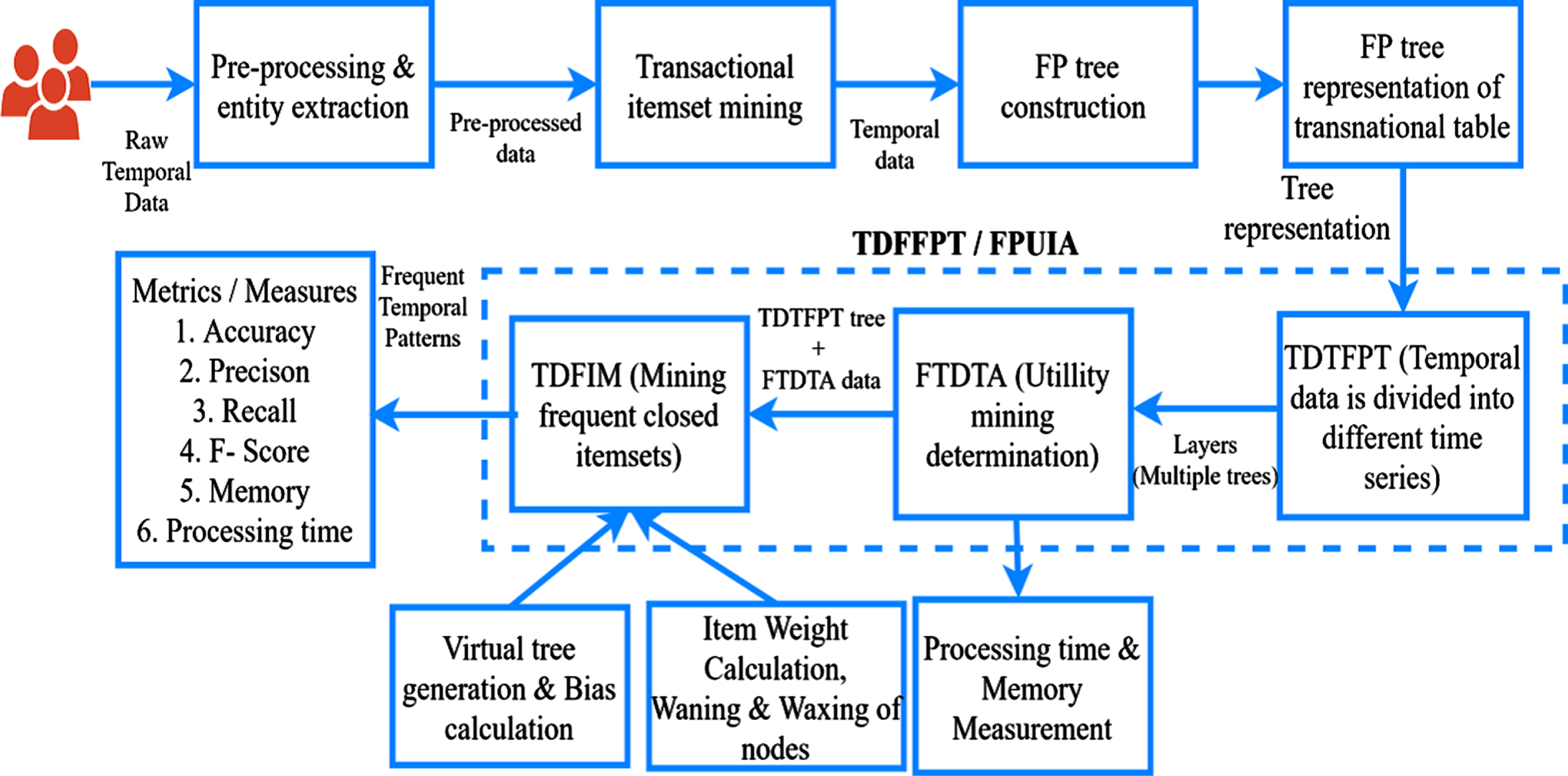
Flow diagram.

5 Experimental setup

A retail temporal dataset with 4995753 number of records entered from 01-01-2010 to 31-12-2018 is downloaded from Amazon to perform the experiments [17]. Experiment is performed with the whole dataset and the performance metrics are logged for every 499575 (10%) records. A computer with Intel Core i5-7200 processor capable of running at 2.7 GHz processing speed equipped with 8GB internal memory is used to carryover the experiments. Windows 10 64-bit operating system is used to run the procedures by a dedicated User Interface (UI) –developed in Visual Studio Integrated Development Environment [18, 19]. RCloud data analytical tool is used to connect with the server to fetch and handle the database [20, 21]. The user interface is capable of accessing the RCloud tool to measure the performance metrics and plot them in graphs for ease of comparison.

Fig. 4

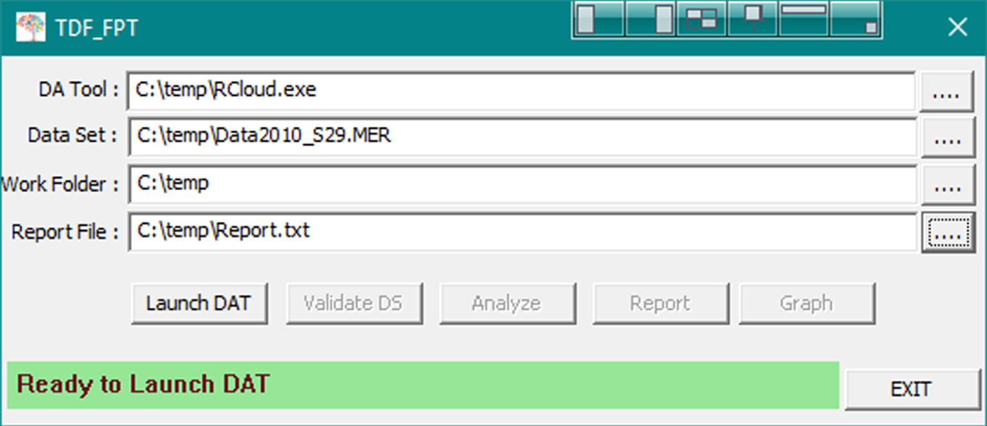
User interface.

6 Results and discussions

Performance metrics such as Accuracy, Precision, Recall, F-Score, Average memory and processing time to process a transaction of discussed method are measured for every 10% of data chuck and presented as Tables and graphs in this section. True Positive (TP), True Negative (TN), False Positive (FP) and False Negative (FN) in the mining activity are measured to calculate the Accuracy, Precision, Recall and F-Score.

6.1 Accuracy

Accuracy is the most expected quality parameter in a data mining procedure. The high value of accuracy represents the high quality of the algorithm. Accuracy is calculated using the formula $\frac{\left(\mathit{TP}+\mathit{TN}\right)}{\left(\mathit{TP}+\mathit{TN}+\mathit{FP}+\mathit{FN}\right)}$ . The measured values of accuracy are given in Fig. 5.

Fig. 5

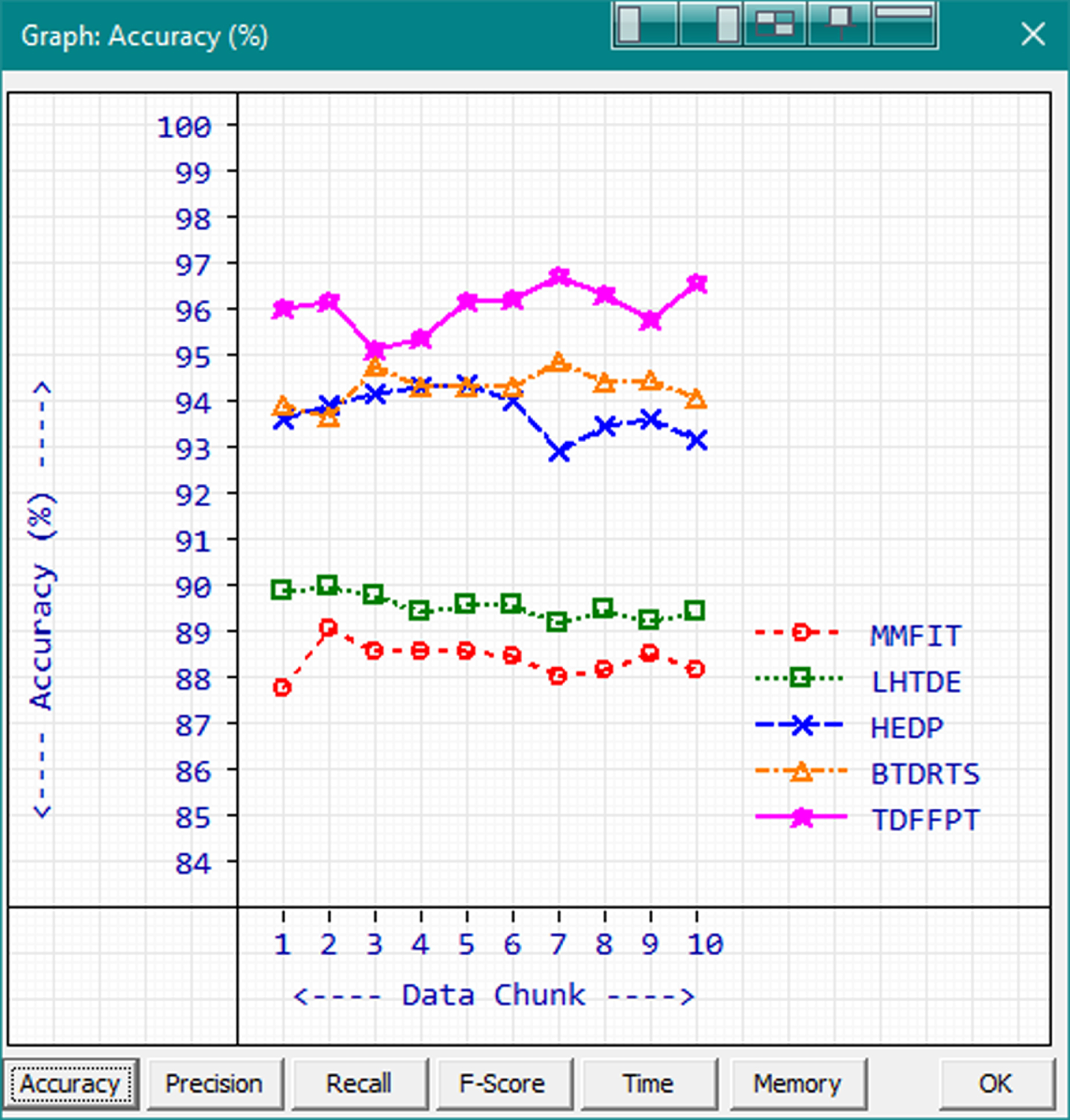
Accuracy.

Based on the observed results, proposed TDFFPT secured more accuracy with the range 95.23% to 96.8% and average 96.15%. BTDRTS, HEDP, LHTDE and MMFIT are getting the accuracy average of 94.41%, 93.86%, 89.64% and 88.5% respectively. The integration of the proposed functional blocks altogether works well to secure high accuracy values in temporal big data mining.

6.2 Precision

Precision is used to refer the closeness of the retrieved information from relevant information. Precision is also treated as important as accuracy in terms of evaluating data mining algorithms. A better-quality data mining should have higher precision values. Precision is calculated by the formula $\frac{\mathit{TP}}{\mathit{TP}+\mathit{FP}}$ . Precision values are measured and produced in Fig. 6.

Fig. 6

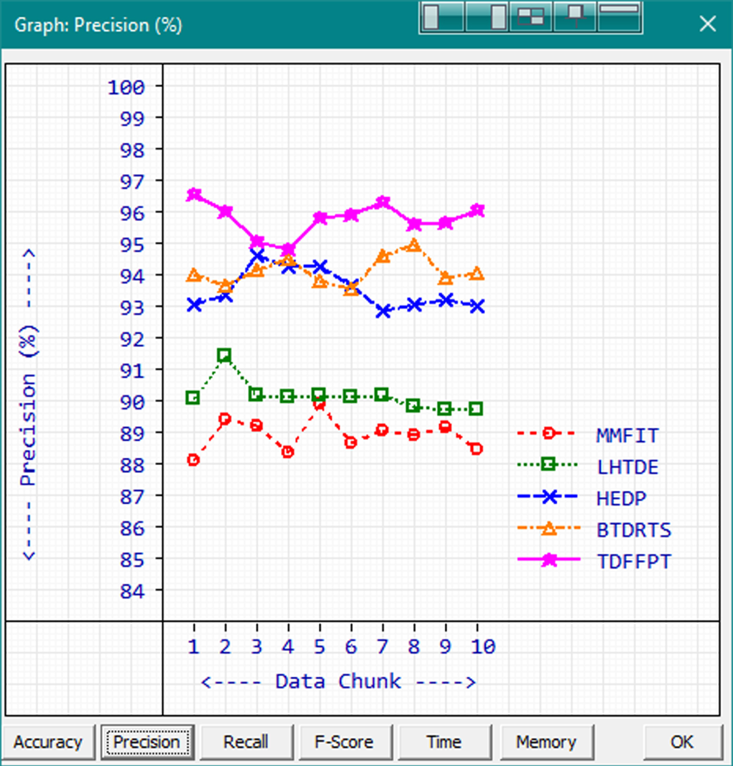
Precision.

Proposed TDFFPT gets the minimum - maximum precision values of 94.92% and 96.66% with the average precision value 95.89%. The highest measured precision value 96.66% is achieved by TDFFPT while processing the first data chunk. The precision value averages of MMFIT, LHTDE, HEDP and BTDRTS are 89.04%, 90.25%, 93.65% and 94.23% respectively. HEDP is performing better than BTDRTS which processing some data chunks and BTDRTS performs better in other data chunks whereas TDFFPT is performing better than both the methods in all data chunks.

6.3 Recall

Recall is the term used to refer the ratio of retrieved relevant instances and overall relevant instances. Similar to accuracy and precision, the high recall value shows the high-quality algorithm. Recall is calculated using the formula $\frac{\mathit{TP}}{\mathit{TP}+\mathit{FN}}$ . Calculated recall values are shown as comparison graph in Fig. 7.

Fig. 7

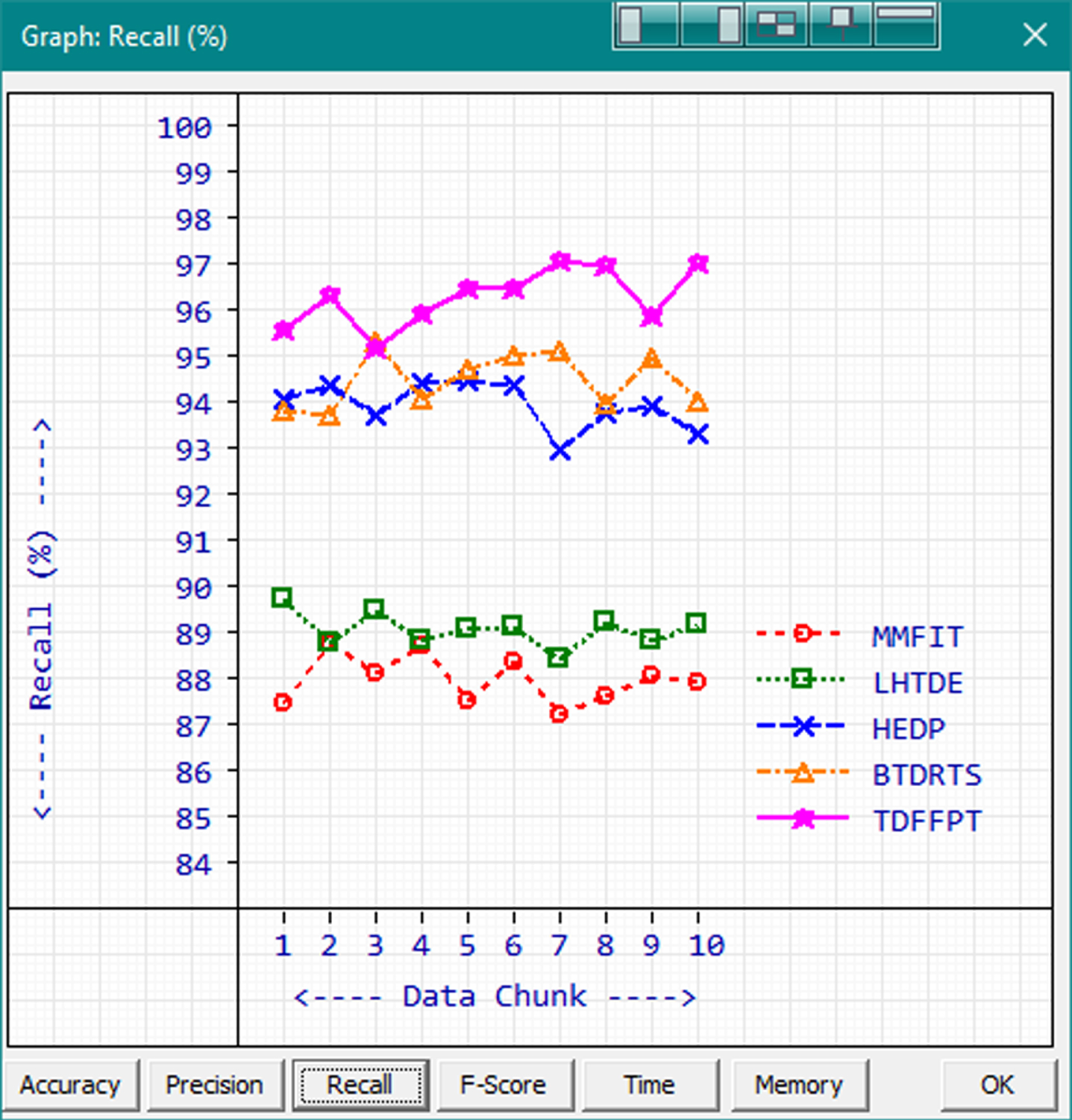
Recall.

The minimum-maximum recall range of TDFFPT is 95.29% to 97.16 with the average of 97.16%. BTDRTS gets the second-high score values with range 93.81% to 95.43% and 94.58% average in terms of recall. HEDP, LHTDE and MMFIT are getting the recall values of 94.04%, 89.16% and 88.08% in order. The highest recall value is achieved by TDFFPT while processing the 7^th data chunk.

6.4 F-score

F-Score is the term used to refer the resonated mean of the precision and recall. F-Score is mainly used to balance the ratio between precision and recall in statistical analysis and machine learning applications. F-Score is calculated by using the formula ${\left(\frac{\mathit{Recal}{l}^{-1}+\mathit{Precisio}{n}^{-1}}{2}\right)}^{-1}$ . The F-Score values of the methods in discussion are given in Fig. 8.

Fig. 8

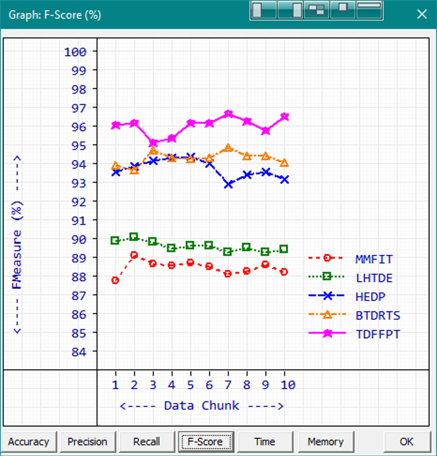
F-Score.

The methods are sorted from best to next based on the F-Score as TDFFPT, BTDRTS, HEDP, LHTDE and MMFIT with the F-Score Averages of 96.14, 94.41, 93.85, 89.71 and 88.58 in order. TDFFPT gets the highest F-Scores in the range from 95.23 to 96.79 with the average of 96.14. The second-best F-Score range is achieved by BTDRTS with the values 93.78 to 94.97.

6.5 Memory

Memory is one of the vital computational resources. A good algorithm should consume most optimum level of memory to avoid overflow issues. Though modern computers come with surplus memory, it is important to use it wisely while handling big data. Memory utilizations of existing and proposed methods are measured and the average memory requirement to handle a record transaction is calculated and shown in Fig. 9.

Fig. 9

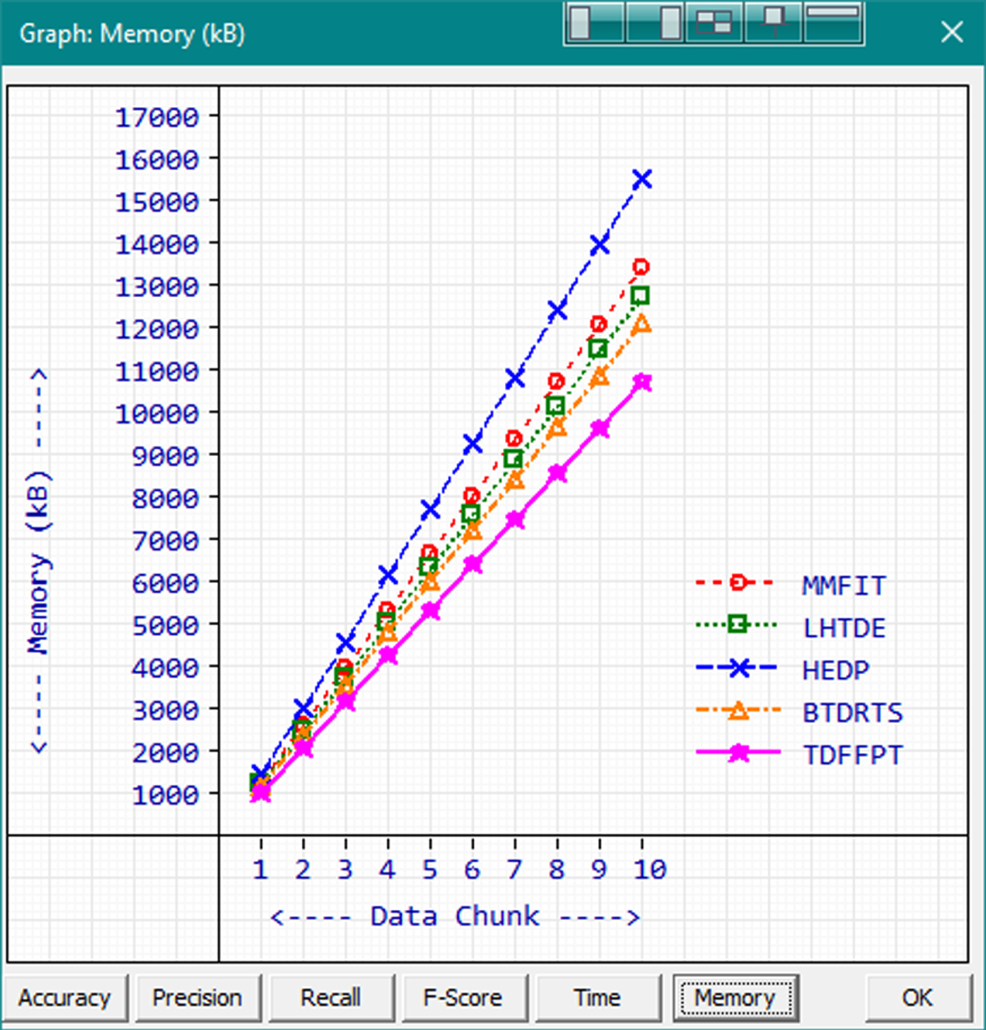
Average memory consumption.

The lower memory requirement shows the better memory management of a data mining procedure. Based on the measured results, proposed TDFFPT consumes lesser memory than the other methods. The memory consumption range of TDFFPT is from 1112 kB to 10802 kB while processing the first data chunk to entire dataset. The next best performer in terms of memory consumption is BTDRTS with the range 1253kB to 12229 kB.

6.6 Processing time

Processing time is the prime characteristic that determines the operational speed of a data mining algorithm. The processing time is measured by calculating the difference between process starting time and completion time. The processing time for 10 data chunks are measured individually and the average processing time to process a record transaction is calculated. The comparison graph is given in Fig. 10.

Fig. 10

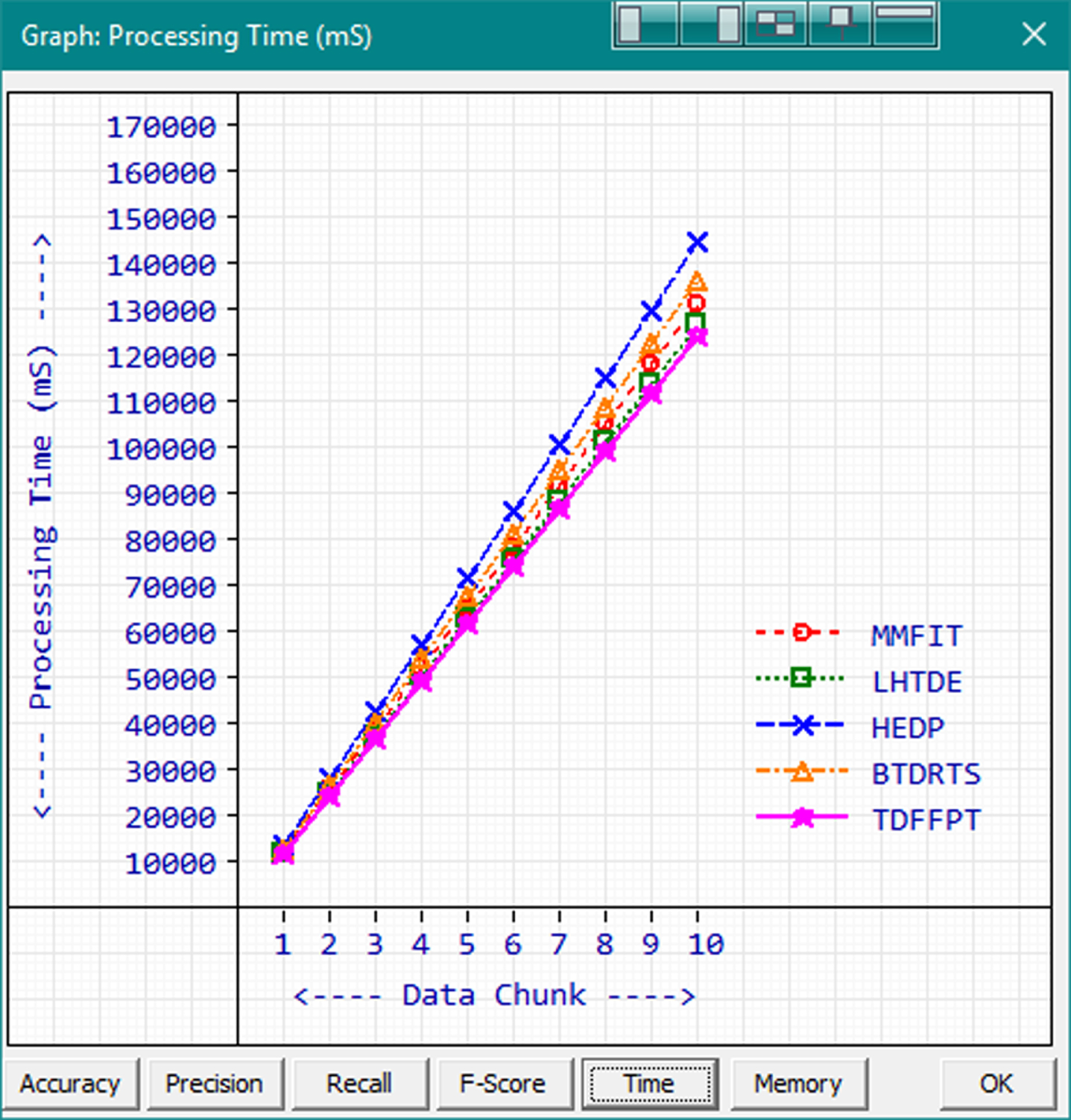
Processing Time(mS).

Based on the measured results, it is observed that the average processing time increases linearly based on the number of records for all methods. The best processing time is 12677 mS achieved by TDFFPT while processing the first data chuck. The processing time of TDFFPT during the 10^th data chunk is 125474 mS. In this case, existing method LHTDE operates slightly faster than BTDRTS with the range 12723 mS to 127541 mS which is in the 2^nd position in the comparison.

7 Conclusion

A Temporal data mining algorithm requires improved data mining characteristics such as accuracy, precision and recall. Modern day connected world produces massive volume of data in the retail domain. Predicting the individual purchase patterns and behavior along with accumulative social consumption demeanor will be more useful to optimize the production and improve profit. The problem in temporal data analysis is the increased computational resource consumption while trying to improve accuracy or the prediction. This problem is well handled by the proposed method which could increase the overall experience by improving the accuracy, precision and recall along with optimized computational resource consumption. The results obtained shows that the performance of the proposed pattern prediction model is more efficient than that of the existing algorithms.

There is also much scope for future work in the form of predictive analysis by combining proposed algorithms with other emerging technologies involving artificial intelligence and machine learning for powerful and accurate data analytics.