Quantitative reachability analysis of generalized possibilistic decision processes

Abstract

The verification of reachability properties of fuzzy systems is usually based on the fuzzy Kripke structure or possibilistic Kripke structure. However, fuzzy Kripke structure or possibilistic Kripke structure is not enough to describe nondeterministic and concurrent fuzzy systems in real life. In this paper, firstly, we propose the generalized possibilistic decision process as the model of nondeterministic and concurrent fuzzy systems, and deduce the possibilities of sets of paths of the generalized possibilistic decision process relying on defining of schedulers. Then, we give fuzzy matrices calculation methods of the maximal possibilities and the minimal possibilities of eventual reachability, always reachability, constrained reachability, repeated reachability and persistent reachability. Finally, we propose a model checking approach to convert the verification of safety property into the analysis of reachabilities.

1 Introduction

Reachability is one of the central problems in model checking [1, 2], program analysis [3] and verification [3], which is about whether a system in one state can reach other states [4]. Reachability is widely applied in urban transportation planning [5], human geography [6], regional economics and computer science [7]. In computer science, the use of reachability decision algorithm can avoid the loop detection of useless state space, save the memory occupancy of the algorithm, and improve the efficiency of the algorithm. The use of reachability optimization algorithm can reduce the complexity of the algorithm [4].

Reachability problems based on classical model checking were proposed in [8]. Classical model checking is to verify the qualitative characteristics of systems. Qualitative reachability aims at obtaining exact values of certain events. However, in real life, there are some randomness, uncertainties and inconsistencies that classical model checking is unable to express those information, such as a 90 percent probability of system crashing during operation [12]. To embed uncertain information into the model, quantitative model checking methods are proposed, including probabilistic model checking [4], possibilistic model checking [17], multi-valued model checking [10, 11] and fuzzy model checking [2, 18]. Quantitative reachability is to find the maximum probability [15] or the minimum probability [17].

This study extends the existing approach of the generalized possibilistic model checking to solve quantitative reachability problems. Li et al. [17, 22] propose possibility model checking and generalized possibility model checking in combination with measure theory, providing a solution to the existing problems of fuzzy model checking. In [17], the reachability problem based on the possibility measure is given, and the reachability problem is studied by using a possibilistic Kripke structure as a model. In the existing generalized possibilistic model checking, the generalized possibilistic Kripke structure is the formal model of the representation system. However, in real life, a generalized possibilistic Kripke structure cannot describe nondeterministic and concurrent fuzzy systems. For example, suppose three experts want to formulate treatment schemes for a new bacterial infection. Because different experts have different understandings of the disease, each expert has a different scheme. We use a generalized possibilistic Kripke structure K = (S, P, I, AP, L) to model the patient’s treatment process respectively. It describes three treatment processes given by three experts(α, β and γ) in Fig. 1(a), (b), (c). However, the generalized possibilistic Kripke structure can only represent the treatment process of a scheme, cannot describe the joint consultation of three experts. To solve this problem, we propose a generalized possibilistic decision process to describe nondeterministic and concurrent fuzzy systems.

Fig. 1

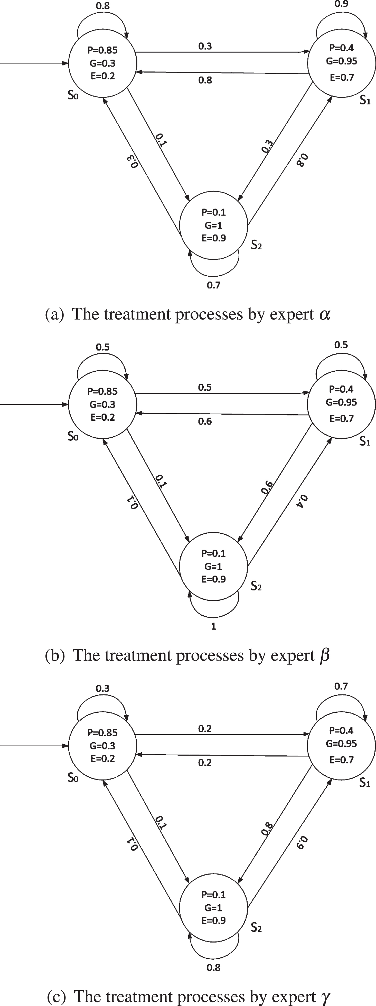
The treatment processes by three experts.

In this paper, we mainly study the maximum possibility problem and the minimum possibility problem of eventual reachability, always reachability, constrained reachability, repeated reachability and persistent reachability under a generalized possibilistic decision process. First, we propose a generalized possibilistic decision process as the model of fuzzy systems, and deduce the possibilities of sets of paths of the generalized possibilistic decision process relying on defining of schedulers. Then, the fuzzy matrices calculation methods of reachability under a generalized possibilistic decision process are given, and the results show that the compositional operations of the fuzzy matrix is polynomial time, which is better than the exponential level of existing algorithms. Finally, we propose a model checking approach to convert the verification of safety property into the analysis of reachabilities.

The rest of this paper is organized as follows. Section 2 gives some preliminary knowledge. In Section 3, we define generalized possibilistic decision processes. In Section 4, we present the fuzzy matrix calculation methods of eventual reachability, always reachability, constrained reachability, repeated reachability and persistent reachability. In Section 5, we use good prefixes to analyze the possibilistic regular safety property. Section 6 is the conclusion. The proofs of some theorems of this paper can be found in the Appendix.

2 Preliminaries

To model and verify fuzzy systems, we provide some necessary knowledge including the fuzzy set, fuzzy set operation, fuzzy matrix operation, closure and others.

Definition 1. [23, 28] Let X be a universal set. A fuzzy set A of X is an function which associates each element in X a value in the interval [0, 1], i.e., A : X ⟶ [0, 1]. For x ∈ X, A (x) is the membership of x in the fuzzy set A.

We use $\mathcal{F}\left(X\right)$ to represent all fuzzy sets in X, i.e. $\mathcal{F}\left(X\right)=\{A\mid A:X⟶[0,1\left]\right\}$ .

Definition 2. [26, 28] Let $A,B\in \mathcal{F}\left(X\right)$ , we use A ∪ B, A ∩ B, A ^c to represent the union, intersection and complement of A and B. The definition is as follows.

(A ∪ B) (x) = A (x) ∨B (x) = max {A (x) , B (x)},

(A ∩ B) (x) = A (x) ∧ B (x) = min {A (x) , B (x)},

A ^c  (x) =1 - A (x).

Definition 3. [26, 28] Let R and S be two fuzzy matrices with m rows and n columns, i.e., R = (r _ij ) _m×n, S = (s _ij ) _m×n. We introduce some set operators.

R = S if and only if r _ij  = s _ij for all i, j.

R ⊆ S if and only if r _ij  ≤ s _ij for all i, j.

R ∪ S = (r _ij ∨s _ij ) _m×n.

R ∩ S = (r _ij  ∧ s _ij ) _m×n.

R ^c  = (1 - r _ij ) _m×n.

Definition 4. [26, 28] Let R be a fuzzy matrix with m rows and n columns, and S be a fuzzy matrix with n rows and l columns, i.e., R = (r _ij ) _m×n and S = (s _ij ) _n×l. The composition operation of R and S is R ∘ S = (t _ij ) _m×l, where $t_{\mathit{ij}}={\vee }_{k=1}^n(r_{\mathit{ik}}\wedge s_{\mathit{kj}})$ , (i = 1, 2, . . . , m, j = 1, 2, . . . , l). For fuzzy matrices R, S, T, the composition operation has some operation laws.

(R ∘ S) ∘ T = R ∘ (S ∘ T);

(R ∪ S) ∘ T = (R ∘ T) ∪ (S ∘ T).

Let X be a universal set. For the fuzzy matrix R = (R (s, t)) _s,t∈X, we use R⁺ to denote its transitive closure. When X is finite, X has ∣X∣ elements, then R⁺ = R ∪ R² ∪ . . . ∪ R^∣X∣, where R^k+1 = R ^k  ∘ R for any positive integer number k. The Kleene closure R^* = R⁰ ∪ R⁺, for each 1≤ s, t ≤ ∣ S ∣, $R^0(s,t)=\{\begin{array}{ccc}\hfill 1& \hfill \hfill & s=t\hfill \\ \hfill 0& \hfill \hfill & s\ne t\hfill \end{array}$ . Possibility measure theory is a kind of uncertainty theory, which mainly deals with incomplete information and uncertain information. In addition, the possibility measure does not require additivity, which is more applicable to deal with practical application systems.

Definition 5. [21] Let X be a nonempty set,and Ω be a set composed of some subsets of X elements. We call Ω a σ- algebra, which is closed to countable and take complement set operations. The possibility measure on σ- algebra Ω is a mapping POS : Ω → [0, 1], which satisfies the following conditions:

POS (∅) =0;

POS (X) =1;

If E _i  ∈ Ω, i ∈ I, then POS (⋃ _i∈IE _i ) = ⋁ _i∈IPOS (E _i )

If only conditions(1) and (3), then POS is called a generalized possibility measure. If POS is a generalized possibility measure on the power set 2 ^X ,for any A ⊆ X, there is POS (A) = ⋁ _a∈APOS ({ a }).

Definition 6. [18] A Generalized possibilistic Kripke structure(GPKS) is a tuple K = (S, P, I, AP, L), where

S is a countable, nonempty states set;

P : S × S → [0, 1] is the possibility transition distribution, for any states s, there is a state t, such that P (s, t) >0;

I : S → [0, 1] is the initial distribution of possibility and there exists a state s, such that I (s) >0;

AP is a set of atomic propositions;

L : S × AP → [0, 1] is a label function, L (s, a) represents the true value of atomic proposition a in state s.

For a GPKS K, its path is defined as an infinite sequence of states π = s₀s₁s₂ ⋯ ∈ s ^ω, for any i so that P (s _i , s_i+1) > 0. Let Paths (s) and Paths _fin  (s) represent the set of all infinite and finite paths starting from the state s in K. Paths (K) represents the set of all infinite paths in K, Paths _fin  (K) represents the set of all finite paths in K, such as $\hat{\pi }=s_0{s}_1\cdots s_n$ .

3 Generalized Possibilistic Decision Processes

In this section, first, we give the notion of the generalized possibilistic decision process. Then, the definition of the scheduler is proposed to solve the nondeterministic the generalized possibilistic decision process. Finally, we solve the generalized possibility measure problems.

Nondeterminism is absent in GPKS. The generalized possibilistic decision process can be viewed as a variant of GPKS that permits both possibility and nondeterministic choices.

Definition 7. A Generalized possibilistic decision process(GPDP) is a tuple M = (S, Act, P, I, AP, L), where

S is a countable, nonempty set of states;

Act is a set of actions;

P : S × Act × S ⟶ [0, 1] is a function, called possibilistic transition distribution function. For all states s ∈ S and actions α ∈ Act, there exits a state t ∈ S such that P (s, α, t) >0;

I : S ⟶ [0, 1] is a function, there exits states s such that I (s) >0;

AP is a set of atomic propositions;

L : S × AP ⟶ [0, 1] is a possibilistic labeling function, which can be viewed as function mapping a state s to the fuzzy set of atomic proposition, L (s, a) denotes the possibility or truth value of atomic proposition a which is hold in state s.

Furthermore, if the set S, Act and AP are finite sets, then M is a finite GPDP. In this paper, we always assume that GPDPs are finite. A GPDP has a unique initial distribution I. For all states s, t ∈ S and actions α ∈ Act, P (s, α, t) denotes the possibility from state s under action α to state t. An action α is enabled in state s if and only if P (s, α, t) >0. Let Act (s) denote the set of enabled actions in state s. For any states s ∈ S, it is required that Act (s)≠ ∅. Each state t for which P (s, α, t) >0 is called an α-successor of s. The set of direct α-successors of s is defined as:

Post (s, α) = {t ∈ S ∣ P (s, α, t) >0}.

The set of α-predecessors of s is defined by:

Pref (t) = {(s, α) ∈ S × Act (s) ∣ P (s, α, t) >0}.

We also use the P (s, α, T) to denote the possibility from the state s under the action α to the set T of states, that is, $P\left(s,\alpha ,T\right)=\underset{t\in T}{\vee }P\left(s,\alpha ,t\right)$ .

Paths in GPDP M are defined as infinite alternating sequences π = s₀ α₀s₁ α₁s₂ ⋯ ∈ (S × Act)  ^ω such that P (s _i , α _i , s_i+1) >0 for all i ∈ I. Paths (s) denotes the set of all infinite paths in M that start in state s. Similarly, Paths _fin  (s) denotes the set of all finite path fragment $\hat{\pi }=s_0{\alpha }_0{s}_1{\alpha }_1{s}_2\cdots {\alpha }_{n-1}{s}_n$ such that s₀ = s. Paths (M) and Paths _fin  (M) denote the set of all infinite paths and finite paths in M respectively. The trace of the infinite path fragment π = s₀s₁⋯ is defined as trace(π) = L (s₀) L (s₁)⋯. The trace of the finite path fragment $\hat{\pi }$ = s₀s₁ ⋯ s _n is defined as trace( $\hat{\pi }$ ) = L (s₀) L (s₁) ⋯ L (s _n ).The trace of all infinite paths starting from state s is defined as Traces (s) = trace (Paths (s)).

Example 1. Let us consider the joint consult of three experts in Fig. 1(a),(b),(c). GPDP in Fig. 2, where states are represented by ovals and transitions by labeled edges, and state names are depicted outside the ovals, and labeling functions of the states are depicted inside the ovals.

Fig. 2

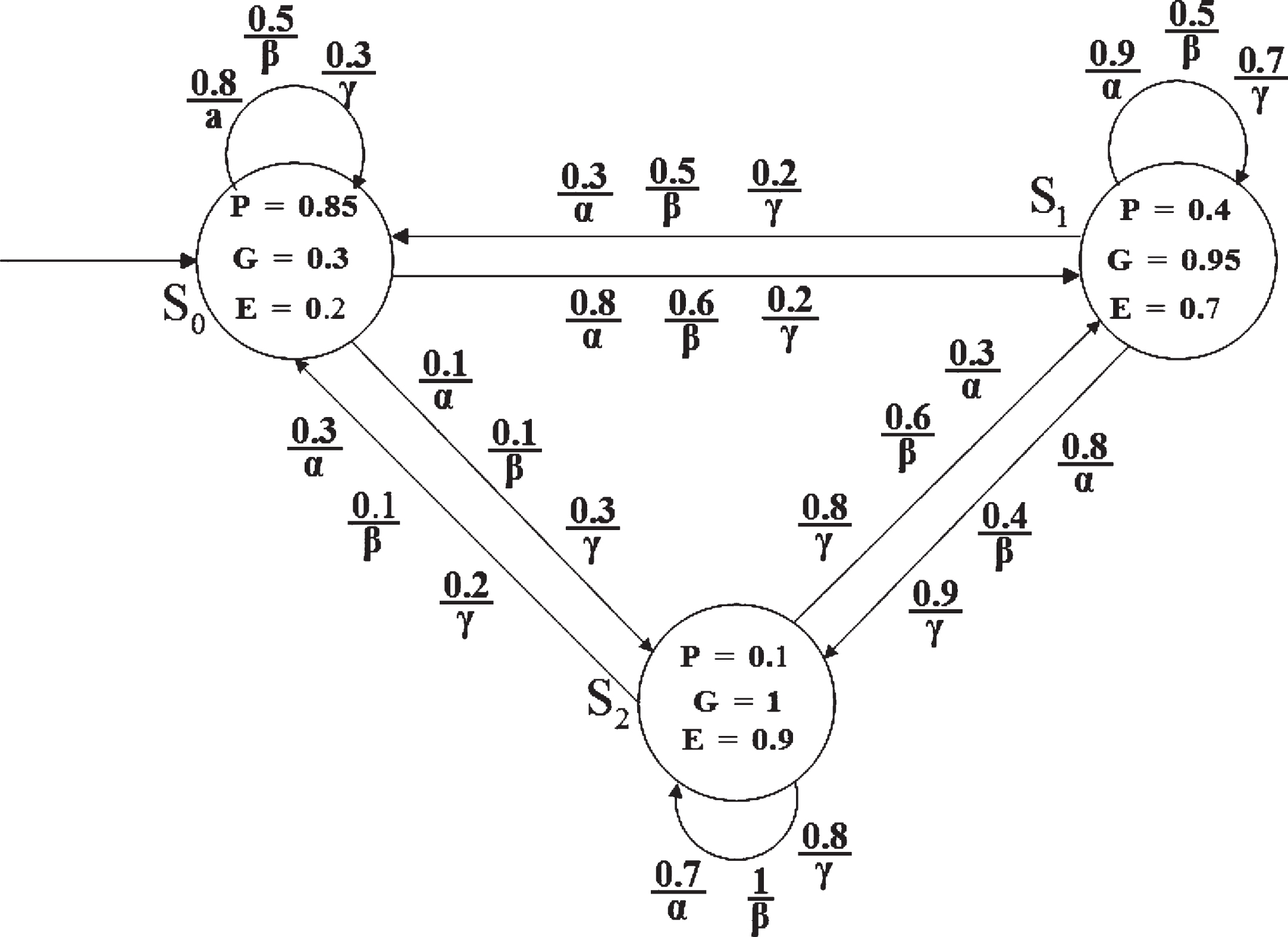
Treatment process by three experts’ consultation.

S = {s₀, s₁, s₂}, Act = {α, β, γ}, AP = {P, G, E}. P indicates that the patient is in “bad” health, G indicates that the patient is in “normal” health, E indicates that the patient is in “good” health.

For state s₀, the labeling functions are L (s₀, P) =0.85, L (s₀, G) =0.3, L (s₀, E) =0.2. L (s₀, P) =0.85 indicates that the degree of “bad” health in state s₀ is 0.85. L (s₀, G) =0.3 indicates that the degree of “normal” health in state s₀ is 0.3. L (s₀, E) =0.2 indicates that the degree of “good” health in state s₀ is 0.2.

Act (s₀) = {α, β, γ}, α, β, γ indicate three different treatment indicates. P (s₀, α, s₁) =0.8 indicates that the possibility of the patient’s health condition changing from state s₀ to state s₁ is 0.8 after the expert treats the patient with the α scheme. P (s₀, β, s₁) =0.6 indicates that the possibility of the patient’s health condition changing from state s₀ to state s₁ is 0.6 after the expert treats the patient with the β scheme. P (s₀, γ, s₁) =0.2 indicates that the possibility of the patient’s health condition changing from state s₀ to state s₁ is 0.2 after the expert treats the patient with the γ scheme.

Post (s₀, α) = {s₁, s₂},Post (s₀, α) indicates all α successor states of state s₀.

Pref (s₀) = {(s₀, α) , (s₀, β) , (s₀, γ) , (s₁, α) , (s₁, β) ,

(s₁, γ) , (s₂, α) , (s₂, β) , (s₂, γ)}, Pref (s₀) indicates all predecessor states of state s₀.

For the GPKS K, 2 ^Paths  (K) is the algebra that is generated by $\left\{\mathit{Cyl}\right(\hat{\pi })\mid \hat{\pi }\in \mathit{Path}{s}_{\mathit{fin}}\left(K\right)\}$ on Paths (K), but the GPDPs are not augmented with a unique possibility measure. Instead, deducing possibilities of sets of paths of a GPDP rely on the resolution of nondeterminism. This resolution is performed by a scheduler. A scheduler chooses in any state s one of the actions set A ⊆ Act (s). It does not impose any constraint on the possibilistic choice that is resolved once α ∈ A has been chosen.

Definition 8. Let M = (S, Act, P, I, AP, L) be a GPDP, a scheduler for M is a function Adv : S → 2 ^Act so that Adv (s) ⊆ Act (s) for all s ∈ S.

Let Path _Adv  (s) and ${\mathit{Path}}_{\mathit{Adv}}^{\mathit{fin}}\left(s\right)$ denote the set of paths and finite paths from state s under the decision of the scheduler Adv. Let Path _Adv  (M) and ${\mathit{Path}}_{\mathit{Adv}}^{\mathit{fin}}\left(M\right)$ denote the set of paths and finite paths in the M under the decision of the scheduler Adv.

Given a GPDP M = (S, Act, P, I, AP, L), α ∈ Act, possibility distribution function P : S × α × S ⟶ [0, 1] can be represented by a fuzzy matrix. For convenience, the fuzzy matrix is written as P _α, so that P _α = (P (s, α, t)) _s,t∈S, called the fuzzy transition matrix of M corresponding to scheduler α. Using fuzzy matrix $P_{\mathit{max}}={\bigvee }_{i=0}^n{P}_{{\alpha }_i}$ denotes the maximal possibility transition matrix, so that ${\left(P_{\mathit{max}}\left(s,t\right)\right)}_{s,t\in S}={\left({\bigvee }_{\alpha \in \mathit{Act}\left(s\right)}P\left(s,\alpha ,t\right)\right)}_{s,t\in S}.$

Using fuzzy matrix $P_{\mathit{min}}={\bigwedge }_{i=0}^n{P}_{{\alpha }_i}$ denotes the minimal possibility transition matrix, so that

${\left(P_{\mathit{min}}\left(s,t\right)\right)}_{s,t\in S}={\left({\bigwedge }_{\alpha \in \mathit{Act}\left(s\right)}P\left(s,\alpha ,t\right)\right)}_{s,t\in S}.$

The GPKS K _max  = (S, P _max , I, AP, L) and GPKS K _min  = (S, P _min , I, AP, L) can be constructed from matrix P _max and matrix P _min respectively.

Example 2. As shown in the Example 1, the order of s₀→s₁→s₂ is used to give the fuzzy matrices P _max , P _min . $\begin{array}{cc}\hfill P_{\mathit{max}}=\left(\begin{array}{ccc}0.8\hfill & 0.8\hfill & 0.3\hfill \\ 0.5\hfill & 0.9\hfill & 0.9\hfill \\ 0.3\hfill & 0.8\hfill & 1\hfill \\ \hfill \end{array}\right),P_{\mathit{min}}=\left(\begin{array}{ccc}0.3\hfill & 0.2\hfill & 0.1\hfill \\ 0.2\hfill & 0.5\hfill & 0.4\hfill \\ 0.1\hfill & 0.3\hfill & 0.7\hfill \\ \hfill \end{array}\right),& \hfill \end{array}$

Figure 3(a) shows the result of GPKS with respect to P _max , Fig. 3(b) shows the result of GPKS with respect to P _min .

Fig. 3

GPKS with respect to P_max and P_min.

Although GPDP can induce the GPKS under the consideration of some schedulers, reasoning about quantitative reachabilities requires a formalization of the possiblities for sets of paths. This formalization is based on possibility measure theory, in particular possibility spaces and generalized possibility measure theory.

Definition 9. Given a GPDP M = (S, Act, P, I, AP, L), let $\hat{\pi }=s_0{\alpha }_0{s}_1{\alpha }_1{s}_2\cdots s_{n-1}{\alpha }_{\mathrm{n}-1}{s}_n\in {\mathit{Paths}}_{\mathit{Adv}}^{\mathit{fin}}\left(M\right)$ and Adv be the max or min scheduler, then the cylinder set of the finite path $\hat{\pi }$ is defined as $\mathit{Cyl}\left(\hat{\pi }\right)=\{\pi \in \mathit{Path}{s}_{\mathit{Adv}}(M)\mid \hat{\pi }\in \mathit{Pref}(\pi \left)\right\},$(1) where $\mathit{Pref}\left({\pi }_{\mathit{Adv}}\right)=\{{\pi }^{\prime }\in {\mathit{Paths}}_{\mathit{Adv}}^{\mathit{fin}}(M)\mid {\pi }^{\prime }$ is a finite prefix of π _Adv }.

The cylinder set spanned by the finite adv-paths $\hat{\pi }$ consists of all infinite adv-paths that start with $\hat{\pi }$ . The cylinder sets serve as basis events of the measurable space 2 ^{Paths _Adv}  (M) associated with M. From classical concepts of possibility theory, it follows that there exists a unique possibility measure GPo on the measurable space 2 ^{Paths _Adv}  (M) associated with M are given by Definition 10.

Definition 10. Let M = (S, Act, P, I, AP, L) be a finite GPDP, the function GPo : Paths _Adv   (M) → [0, 1] is defined:

$\mathit{GPo}\left(\pi \right)=I\left(s_0\right)\wedge \underset{i\ge 0}{\wedge }{P}_{\mathit{Adv}}(s_i,{\alpha }_i,s_{i+1})$(2) where π = s₀ α₀s₁ α₁s₂ ⋯ ∈ Paths _Adv   (M). Furthermore, we define GPo (E) = ∨ {GPo (π) ∣ π ∈ E}, for any E ⊆ Paths _Adv   (M), then we have the function $\mathit{GPo}:2^{\mathit{Path}{s}_{\mathit{Adv}}\left(M\right)}\to [0,1]$ is called generalized possibility measure over Ω = 2^{Paths _Adv (M)}.

Let M = (S, Act, P, I, AP, L) be a GPDP, s ∈ S, α _i  ∈ Act, i ≥ 0, r _Adv  : S → [0, 1] is defined as following, which denotes the maximal possibility measure of all Adv-paths from state s in M:

$\begin{array}{cc}\hfill r_{\mathit{Adv}}\left(s\right)=& \bigvee \left\{{\bigwedge }_{i\ge 0}{P}_{\mathit{Adv}}\right(s_i,{\alpha }_i,s_{i+1})\mid s_1\hfill \\ \hfill & =s,s_i\in S,{\alpha }_i\in \mathit{Act}\}.\hfill \end{array}$(3)

The role of the function r _Adv is to help us to calculate the possibility of Adv-paths in M. The Theorem 1 gives a fuzzy matrix calculation for r _Adv .

Theorem 1. Let M = (S, Act, P, I, AP, L) be a finite GPDP, for any s ∈ S, then we have

$r_{\mathit{Adv}}\left(s\right)=\underset{t\in S}{\bigvee }\left(P_{\mathit{Adv}}^{+}(s,t)\wedge P_{\mathit{Adv}}^{+}(t,t)\right).$(4)

In particular, P _Adv is normal iff r _Adv  (s) =1 for any states s.

Proof. See the Appendix. ■

In the matrix notation, we have

$r_{\mathit{Adv}}=P_{\mathit{Adv}}^{+}\circ D_{\mathit{Adv}},$(5) where $D_{\mathit{Adv}}={\left(P_{\mathit{Adv}}^{+}\left(t,t\right)\right)}_{t\in S}$ .

The computational complexity of r _Adv  (s) mainly depends on the time of computational possibilistic transition closure. In [30], they gave an optimal algorithm to calculate D _Adv , then we get the time complexity is O (n² log n), where n =∣ S ∣.

Example 3. According to the GPDP in Example 1, for any s ∈ S,r _max and r _min corresponding to the maximal scheduler and the minimal scheduler are given,

$D_{\mathit{max}}={\left(P_{\mathit{max}}^{+}\left(t,t\right)\right)}_{t\in S}=\left(\begin{array}{c}\hfill 0.8\hfill \\ \hfill 0.9\hfill \\ \hfill 1\hfill \end{array}\right),$

$D_{\mathit{min}}={\left(P_{\mathit{min}}^{+}\left(t,t\right)\right)}_{t\in S}=\left(\begin{array}{c}\hfill 0.3\hfill \\ \hfill 0.5\hfill \\ \hfill 0.7\hfill \end{array}\right),$

$P_{\mathit{max}}^{+}=\left(\begin{array}{ccc}\hfill 0.8\hfill & \hfill 0.8\hfill & \hfill 0.8\hfill \\ \hfill 0.5\hfill & \hfill 0.9\hfill & \hfill 0.9\hfill \\ \hfill 0.5\hfill & \hfill 0.8\hfill & \hfill 1\hfill \\ \hfill \hfill \end{array}\right),$

$P_{\mathit{min}}^{+}=\left(\begin{array}{ccc}\hfill 0.3\hfill & \hfill 0.2\hfill & \hfill 0.1\hfill \\ \hfill 0.2\hfill & \hfill 0.5\hfill & \hfill 0.4\hfill \\ \hfill 0.2\hfill & \hfill 0.3\hfill & \hfill 0.7\hfill \\ \hfill \hfill \end{array}\right),$

$r_{\mathit{max}}=P_{\mathit{max}}^{+}\circ D_{\mathit{max}}=\left(\begin{array}{c}\hfill 0.8\hfill \\ \hfill 0.9\hfill \\ \hfill 1\hfill \end{array}\right),$

$r_{\mathit{min}}=P_{\mathit{min}}^{+}\circ D_{\mathit{min}}=\left(\begin{array}{c}\hfill 0.3\hfill \\ \hfill 0.5\hfill \\ \hfill 0.7\hfill \end{array}\right).$

r _max  (s₀) = 0.8 indicates that under the maximal possibilistic scheduler. That is, the maximal possibility of all paths from state s₀ is 0.8. r _min  (s₀) = 0.3 indicates that under the minimal possibilistic scheduler. That is, the maximal possibility of all paths from state s₀ is 0.3.

Based on Theorem 1, we can get Theorem 2, which can convert the calculation of generalized possibility measure of infinite path into the calculation of possibility of finite path.

Theorem 2. Let M = (S, Act, P, I, AP, L) be a finite GPDP, then the generalized possibility measure of cylinder set $\hat{\pi }=s_0{\alpha }_0{s}_1{\alpha }_1\cdots {\alpha }_{n-1}{s}_n\in {\mathit{Paths}}_{\mathit{Adv}}^{\mathit{fin}}\left(M\right)$ is: $\begin{array}{cc}\hfill & \mathit{GPo}\left(\mathit{Cyl}(s_0{\alpha }_0{s}_1{\alpha }_1\cdots {\alpha }_{n-1}{s}_n)\right)\hfill \\ \hfill & =I\left(s_0\right)\wedge \underset{i=0}{\overset{n-1}{\wedge }}{P}_{\mathit{Adv}}\left(s_i,{\alpha }_i,s_{i+1}\right)\wedge r_{\mathit{Adv}}\left(s_n\right),\hfill \end{array}$ where GPo (Cyl (s₀)) = I (s₀) ∧ r _Adv  (s₀).

Proof. See the Appendix. ■

Example 4. According to the GPDP of Example 1, under the maximal possibilistic measure and the minimal possibilistic measure, the generalized possibility measure of cylinder set of the corresponding finite paths $\hat{\pi }=s_0{\alpha }_0{s}_1$ are respectively,

GPo _max  (Cyl (s₀ α₀s₁) ) = I (s₀) ∧ P (s₀, α₀, s₁) ∧ r _max  (s₁) =0.8

GPo _min  (Cyl (s₀ α₀s₁)) = I (s₀) ∧ P (s₀, α₀, s₁) ∧ r _min  (s₁) =0.5 .

4 Reachability possibility

A typical task for the quantitative analysis of GPDPs is to compute the minimum or the maximum possibility for some reachabilities under consideration of the min or the max scheduler. This corresponds to the worst-case or best-case analysis possibility of GPDPs. Let M = (S, Act, P, I, AP, L) be a finite GPDP and B be a fuzzy set of target states. The fuzzy set B may represent a set of certain bad states that shall be visited with the minimum possibility, or dually, a set of good states that shall be visited with the maximum possibility. Some special reachabilities, such as eventual reachability, always reachability, constrained reachability, repeated reachability and persistent reachability are considered in this section.

4.1 Eventual reachability possibility

The event of eventual reachability is denoted ⋄B. We use the B : S ⟶ [0, 1] to represent the fuzzy set of states. For the given GPDP M, π = s₀ α₀s₁ … ∈ Paths _Adv  (M), ∣∣ ⋄ B (π) ∣∣ = ⋁ _i≥0B (s _i ). In the following, the quantitative analysis of eventual reachability is reduced to the computational range for all strategies of the minimum possibility or the maximum possibility of reaching a certain fuzzy set B of states.

Theorem 3. Let M = (S, Act, P, I, AP, L) be GPDP, max corresponds to the maximum possibility scheduler and min corresponds to the minimum possibility scheduler, then we have, $\begin{array}{cc}\hfill {\mathit{GPo}}_{\mathit{max}}(\diamond B)& =({\mathit{GPo}}_{\mathit{max}}(s\models \diamond B){)}_{s\in S}\hfill \\ \hfill & =P_{\mathit{max}}^{*}\circ D_B\circ r_{\mathit{max}}\hfill \end{array}$(6) $\begin{array}{cc}\hfill {\mathit{GPo}}_{\mathit{min}}(\diamond B)& =({\mathit{GPo}}_{\mathit{min}}(s\models \diamond B){)}_{s\in S}\hfill \\ \hfill & =P_{\mathit{min}}^{*}\circ D_B\circ r_{\mathit{min}}.\hfill \end{array}$(7)

Proof. See the Appendix. ■

Example 5. Based on Example 1, consider the generalized possibility of eventual reachability event ⋄B. Given the fuzzy state set B = (L (s, E)) _s∈S, only the reachability of the event is considered at this point, and the label function in GPDP is defined as L (s) = s.

Then the maximum possibility and minimum possibility of the event ◊^≤7B are respectively: $\begin{array}{cc}\hfill & {\mathit{GPo}}_{\mathit{max}}\left({◊}^{\le 7}B\right)=P_{\mathit{max}}^{*}\circ D_B\circ r_{\mathit{max}}\hfill \\ \hfill & ={\left(\begin{array}{ccc}\hfill 0.8\hfill & \hfill 0.8\hfill & \hfill 0.3\hfill \\ \hfill 0.5\hfill & \hfill 0.9\hfill & \hfill 0.9\hfill \\ \hfill 0.3\hfill & \hfill 0.8\hfill & \hfill 1\hfill \\ \hfill \hfill \end{array}\right)}^{*}\circ \left(\begin{array}{ccc}\hfill 0.2\hfill & \hfill 0\hfill & \hfill 0\hfill \\ \hfill 0\hfill & \hfill 0.7\hfill & \hfill 0\hfill \\ \hfill 0\hfill & \hfill 0\hfill & \hfill 0.9\hfill \\ \hfill \hfill \end{array}\right)\circ \left(\begin{array}{c}\hfill 0.8\hfill \\ \hfill 0.9\hfill \\ \hfill 1\hfill \end{array}\right)\hfill \\ \hfill & =\left(\begin{array}{c}\hfill 0.8\hfill \\ \hfill 0.9\hfill \\ \hfill 0.9\hfill \end{array}\right),\hfill \end{array}$ $\begin{array}{cc}\hfill & {\mathit{GPo}}_{\mathit{min}}\left({◊}^{\le 7}B\right)=P_{\mathit{min}}^{*}\circ D_B\circ r_{\mathit{min}}\hfill \\ \hfill & ={\left(\begin{array}{ccc}\hfill 0.2\hfill & \hfill 0.3\hfill & \hfill 0.1\hfill \\ \hfill 0.2\hfill & \hfill 0.5\hfill & \hfill 0.4\hfill \\ \hfill 0.1\hfill & \hfill 0.3\hfill & \hfill 0.7\hfill \\ \hfill \hfill \end{array}\right)}^{*}\circ \left(\begin{array}{ccc}\hfill 0.2\hfill & \hfill 0\hfill & \hfill 0\hfill \\ \hfill 0\hfill & \hfill 0.7\hfill & \hfill 0\hfill \\ \hfill 0\hfill & \hfill 0\hfill & \hfill 0.9\hfill \\ \hfill \hfill \end{array}\right)\circ \left(\begin{array}{c}\hfill 0.3\hfill \\ \hfill 0.5\hfill \\ \hfill 0.7\hfill \end{array}\right)\hfill \\ \hfill & =\left(\begin{array}{c}\hfill 0.2\hfill \\ \hfill 0.5\hfill \\ \hfill 0.7\hfill \end{array}\right).\hfill \end{array}$

∥GPo (◊ ^≤7B) ∥  _max  (s₀) =0.8, ∥GPo (◊ ^≤7B) ∥  _min  (s₀) =0.2, describes the maximum possibility of the patient’s final state of health with the maximum possibility of “good” being 0.8 and the minimum possibility of “good” being 0.2 after 7 days treatment from state s₀.

4.2 Always reachability possibility

The event of always reachability is denoted B. We use the B : S ⟶ [0, 1] to represent the fuzzy set of states. For the given GPDPs M, π = s₀ α₀s₁ … ∈ Paths _Adv  (M), B (π) = ⋀ _i≥0B (s _i ). Under the maximum possibility scheduler and the minimum possibility scheduler, the methods of computing GPo _max  (s ⊨  B) and GPo _min  (s ⊨  B) are given. $\begin{array}{cc}\hfill & {\mathit{GPo}}_{\mathit{max}}(s\models B)\hfill \\ \hfill & ={\bigvee }_{\pi \in {\mathit{Paths}}_{\mathit{max}}\left(s\right)}({\mathit{GPo}}_{\mathit{max}}\left(\pi \right)\wedge \parallel B\parallel \left(\pi \right))\hfill \\ \hfill & =\bigvee ({\mathit{GPo}}_{\mathit{max}}\left(\pi \right)\wedge {\bigwedge }_{i\ge 0}B\left(s_i\right)).\hfill \end{array}$

$\begin{array}{cc}\hfill & {\mathit{GPo}}_{\mathit{min}}(s\models B)=\bigvee ({\mathit{GPo}}_{\mathit{min}}\left(\pi \right)\wedge \parallel B\parallel \left(\pi \right))\hfill \\ \hfill & =\bigvee ({\mathit{GPo}}_{\mathit{min}}\left(\pi \right)\wedge {\bigwedge }_{i\ge 0}B\left(s_i\right)).\hfill \end{array}$ From these results, we can get Theorem 4.

Theorem 4. Let M = (S, Act, P, I, AP, L) be GPDPs, max corresponds to the maximum possibility scheduler and min corresponds to the minimum possibility scheduler, then we have

$\begin{array}{cc}\hfill {\mathit{GPo}}_{\mathit{max}}\left(B\right)& =\left({\mathit{GPo}}_{\mathit{max}}\right(s\models B){)}_{s\in S}\hfill \\ \hfill & =\upsilon .f_{\mathit{Bmax}}\left(Z\right),\hfill \end{array}$(8)

$\begin{array}{cc}\hfill {\mathit{GPo}}_{\mathit{min}}\left(B\right)& =\left({\mathit{GPo}}_{\mathit{min}}\right(s\models B){)}_{s\in S}\hfill \\ \hfill & =\upsilon .f_{\mathit{Bmin}}\left(Z\right),\hfill \end{array}$(9) where f _Bmax  (Z) = B ∧ P _max  ∘ D _Z  ∘ r _max , f _Bmin  (Z) = B ∧ P _min  ∘ D _Z  ∘ r _min . υ . f _Bmax  (Z) denotes the maximal fixed point of the operator f _Bmax  (Z), υ . f _Bmin  (Z) denotes the minimal fixed point of the operator f _Bmin  (Z). We have given the solution to the maximal fixed point in [18].

Example 6. Based on Example 1, considering the generalized possibility of always reachability event ^≤7B, given the fuzzy state set B = (L (s, E)) _s∈S, the maximum possibility and the minimum possibility of all states in M satisfied event ^≤7B are respectively:

$\begin{array}{cc}\hfill & f\left(z_1\right)=B\wedge (P_{\mathit{max}}^{*}\circ D_z\circ r_{\mathit{max}})\hfill \\ \hfill & =\left(\begin{array}{c}\hfill 0.2\hfill \\ \hfill 0.7\hfill \\ \hfill 0.9\hfill \end{array}\right)\wedge \hfill \\ \hfill & \left({\left(\begin{array}{cccc}\hfill \hfill & \hfill 0.8\hfill & \hfill 0.8\hfill & \hfill 0.3\hfill \\ \hfill \hfill & \hfill 0.5\hfill & \hfill 0.9\hfill & \hfill 0.9\hfill \\ \hfill \hfill & \hfill 0.3\hfill & \hfill 0.8\hfill & \hfill 1\hfill \\ \hfill \hfill \end{array}\right)}^{*}\circ \left(\begin{array}{cccc}\hfill \hfill & \hfill 1\hfill & \hfill 0\hfill & \hfill 0\hfill \\ \hfill \hfill & \hfill 0\hfill & \hfill 1\hfill & \hfill 0\hfill \\ \hfill \hfill & \hfill 0\hfill & \hfill 0\hfill & \hfill 1\hfill \\ \hfill \hfill \end{array}\right)\circ \left(\begin{array}{c}\hfill 0.8\hfill \\ \hfill 0.9\hfill \\ \hfill 1\hfill \end{array}\right)\right)\hfill \\ \hfill & =\left(\begin{array}{c}\hfill 0.2\hfill \\ \hfill 0.7\hfill \\ \hfill 0.9\hfill \end{array}\right),\hfill \end{array}$

$\begin{array}{cc}\hfill & f\left(z_2\right)=B\wedge (P_{\mathit{max}}^{*}\circ D_{z_1}\circ r_{\mathit{max}})\hfill \\ \hfill & =\left(\begin{array}{c}\hfill 0.2\hfill \\ \hfill 0.7\hfill \\ \hfill 0.9\hfill \end{array}\right)\wedge \hfill \\ \hfill & \left({\left(\begin{array}{ccc}\hfill 0.8\hfill & \hfill 0.8\hfill & \hfill 0.3\hfill \\ \hfill 0.5\hfill & \hfill 0.9\hfill & \hfill 0.9\hfill \\ \hfill 0.3\hfill & \hfill 0.8\hfill & \hfill 1\hfill \\ \hfill \hfill \end{array}\right)}^{*}\circ \left(\begin{array}{ccc}\hfill 0.2\hfill & \hfill 0\hfill & \hfill 0\hfill \\ \hfill 0\hfill & \hfill 0.7\hfill & \hfill 0\hfill \\ \hfill 0\hfill & \hfill 0\hfill & \hfill 0.9\hfill \\ \hfill \hfill \end{array}\right)\circ \left(\begin{array}{c}\hfill 0.8\hfill \\ \hfill 0.9\hfill \\ \hfill 1\hfill \end{array}\right)\right)\hfill \\ \hfill & =\left(\begin{array}{c}\hfill 0.2\hfill \\ \hfill 0.7\hfill \\ \hfill 0.9\hfill \end{array}\right).\hfill \end{array}$

fz₁ = fz₂, Therefore $\begin{array}{cc}\hfill {\mathit{GPo}}_{\mathit{max}}\left(\le 7B\right)=\left(\begin{array}{c}\hfill 0.2\hfill \\ \hfill 0.7\hfill \\ \hfill 0.9\hfill \end{array}\right).& \hfill \end{array}$

Calculated by the same method $\begin{array}{cc}\hfill {\mathit{GPo}}_{\mathit{min}}\left(\le 7B\right)=\left(\begin{array}{c}\hfill 0.2\hfill \\ \hfill 0.5\hfill \\ \hfill 0.7\hfill \end{array}\right).& \hfill \end{array}$

∥GPo ( E) ∥  _max  (s₀) =0.2, ∥GPo ( E) ∥  _min  (s₀) =0.2, it shows that from the state s₀, it is unlikely that the patient’s health always reach a “good” state after 7 days treatment.

4.3 Constrained reachability possibility

Given the GPDP M, and the fuzzy set of states B, C : S ⟶ [0, 1], consider the event of reaching B via a finite path fragment which ends in a fuzzy state s ∈ B, and visits only states in set of fuzzy states C prior to reaching fuzzy states s. This event is denoted by C ⊔ B. For n ≥ 0, the event C ⊔ ^≤nB has the same meaning as C ⊔ B, and it is required to reach B(via fuzzy state C) within n steps. Formally, C ⊔ ^≤nB is the union of the basic cylinders spanned by path fragments s₀ α₀s₁ α₁ … s _m so that m ≤ n with possibility C (s _i ) for all 0 ≤ i ≤ m with possibility B (s _k ).

Theorem 5. Let M = (S, Act, P, I, AP, L) be a GPDP, max corresponds to the maximum possibility scheduler and min corresponds to the minimum possibility scheduler, then we have

$\begin{array}{cc}\hfill {\mathit{GPo}}_{\mathit{max}}\left(C{\bigsqcup }^{\le n}B\right)={\mathit{GPo}}_{\mathit{max}}(C\bigsqcup B)& \hfill \\ \hfill =(D_C\circ P_{\mathit{max}}{)}^{*}\circ D_B\circ r_{\mathit{max}},& \hfill \end{array}$(10)

$\begin{array}{cc}\hfill {\mathit{GPo}}_{\mathit{min}}\left(C{\bigsqcup }^{\le n}B\right)={\mathit{GPo}}_{\mathit{min}}(C\bigsqcup B)& \hfill \\ \hfill =(D_C\circ P_{\mathit{min}}{)}^{*}\circ D_B\circ r_{\mathit{min}}.& \hfill \end{array}$(11)

Proof. See the Appendix. ■

Example 7. Next, let’s continue to consider the generalized possibility of constrained reachability event C ⊔ ^≤7B. Given the fuzzy state set C = (L (s, P)) _s∈S, B = (L (s, E)) _s∈S, the maximum possibility and the minimum possibility of all states in M satisfying event C ⊔ ^≤7B are respectively:

$\begin{array}{cc}\hfill & {\mathit{GPo}}_{\mathit{max}}\left(C{\bigsqcup }^{\le 7}B\right)=(D_C\circ P_{\mathit{max}}{)}^{*}\circ D_B\circ r_{\mathit{max}}\hfill \\ \hfill & ={\left(\left(\begin{array}{ccc}\hfill 0.85\hfill & \hfill 0\hfill & \hfill 0\hfill \\ \hfill 0\hfill & \hfill 0.4\hfill & \hfill 0\hfill \\ \hfill 0\hfill & \hfill 0\hfill & \hfill 0.1\hfill \\ \hfill \hfill \end{array}\right)\circ \left(\begin{array}{ccc}\hfill 0.8\hfill & \hfill 0.8\hfill & \hfill 0.3\hfill \\ \hfill 0.5\hfill & \hfill 0.9\hfill & \hfill 0.9\hfill \\ \hfill 0.3\hfill & \hfill 0.8\hfill & \hfill 1\hfill \\ \hfill \hfill \end{array}\right)\right)}^{*}\hfill \\ \hfill & \circ \left(\begin{array}{ccc}\hfill 0.2\hfill & \hfill 0\hfill & \hfill 0\hfill \\ \hfill 0\hfill & \hfill 0.7\hfill & \hfill 0\hfill \\ \hfill 0\hfill & \hfill 0\hfill & \hfill 0.9\hfill \\ \hfill \hfill \end{array}\right)\circ \left(\begin{array}{c}\hfill 0.8\hfill \\ \hfill 0.9\hfill \\ \hfill 1\hfill \end{array}\right)\hfill \\ \hfill & =\left(\begin{array}{c}\hfill 0.7\hfill \\ \hfill 0.7\hfill \\ \hfill 0.9\hfill \end{array}\right),\hfill \end{array}$ $\begin{array}{cc}\hfill & {\mathit{GPo}}_{\mathit{min}}\left(C{\bigsqcup }^{\le 7}B\right)=(D_C\circ P_{\mathit{min}}{)}^{*}\circ D_B\circ r_{\mathit{min}}\hfill \\ \hfill & ={\left(\left(\begin{array}{ccc}\hfill 0.85\hfill & \hfill 0\hfill & \hfill 0\hfill \\ \hfill 0\hfill & \hfill 0.4\hfill & \hfill 0\hfill \\ \hfill 0\hfill & \hfill 0\hfill & \hfill 0.1\hfill \\ \hfill \hfill \end{array}\right)\circ \left(\begin{array}{ccc}\hfill 0.2\hfill & \hfill 0.3\hfill & \hfill 0.1\hfill \\ \hfill 0.2\hfill & \hfill 0.5\hfill & \hfill 0.4\hfill \\ \hfill 0.1\hfill & \hfill 0.3\hfill & \hfill 0.7\hfill \\ \hfill \hfill \end{array}\right)\right)}^{*}\hfill \\ \hfill & \circ \left(\begin{array}{ccc}\hfill 0.2\hfill & \hfill 0\hfill & \hfill 0\hfill \\ \hfill 0\hfill & \hfill 0.7\hfill & \hfill 0\hfill \\ \hfill 0\hfill & \hfill 0\hfill & \hfill 0.9\hfill \\ \hfill \hfill \end{array}\right)\circ \left(\begin{array}{c}\hfill 0.3\hfill \\ \hfill 0.5\hfill \\ \hfill 0.7\hfill \end{array}\right)\hfill \\ \hfill & =\left(\begin{array}{c}\hfill 0.2\hfill \\ \hfill 0.5\hfill \\ \hfill 0.7\hfill \end{array}\right).\hfill \end{array}$

∥GPo (C ⊔ ^≤7B) ∥  _max  (s₀) =0.7, ∥GPo (C ⊔ ^≤7B) ∥  _min  (s₀) =0.2, which means that the patient’s health state is “bad” at state s₀. The expert adopts three treatment schemes after 7 days of treatment, the maximum possibility that a patient’s health states turn to a “good” state is 0.7 and the minimum possibility is 0.2.

4.4 Repeated reachability possibility

Let B : S ⟶ [0, 1] be a set of fuzzy states in GPDPs. For the event of repeated reachability, we use the  ⋄ B to represent it. The set of all paths that visit B infinitely is often measurable. Let π = s₀ α₀s₁ α₁ … ∈ Paths _Adv  (s₀), $\parallel \diamond B\parallel \left(\pi \right)={\bigvee }_{i\ge 0}^{\infty }{\bigwedge }_{j\ge i}^{\infty }B\left(s_j\right)$ , we consider to calculate GPo _Adv  (s ⊨  ⋄ B) under a scheduler Adv.

Theorem 6. Let M = (S, Act, P, I, AP, L) be a GPDP, B : S ⟶ [0, 1] is a fuzzy set of states, max corresponds to the maximum possibility scheduler and min corresponds to the minimum possibility scheduler. Then we have,

$\begin{array}{cc}\hfill {\mathit{GPo}}_{\mathit{max}}(\diamond B)=P_{\mathit{max}}^{+}\circ \mathit{diag}\left(P_{\mathit{max}}^{+}\right(t,t){)}_{t\in S}\circ B,& \hfill \end{array}$(12)

$\begin{array}{cc}\hfill {\mathit{GPo}}_{\mathit{min}}(\diamond B)=P_{\mathit{min}}^{+}\circ \mathit{diag}\left(P_{\mathit{min}}^{+}\right(t,t){)}_{t\in S}\circ B.& \hfill \end{array}$(13)

Proof. See the Appendix. ■

Example 8. Next, let’s continue to consider the generalized possibility of the repeated reachability event  ⋄ B. Given the fuzzy state set B = (L (s, P)) _s∈S, the maximum possibility and the minimum possibility of all states in M satisfying event  ⋄ B are respectively:

$\begin{array}{cc}\hfill & {\mathit{GPo}}_{\mathit{max}}(\diamond B)=P_{\mathit{max}}^{+}\circ \mathit{diag}\left(P_{\mathit{max}}^{+}\right(t,t){)}_{t\in S}\circ B\hfill \\ \hfill & ={\left(\begin{array}{ccc}\hfill 0.8\hfill & \hfill 0.8\hfill & \hfill 0.3\hfill \\ \hfill 0.5\hfill & \hfill 0.9\hfill & \hfill 0.9\hfill \\ \hfill 0.3\hfill & \hfill 0.8\hfill & \hfill 1\hfill \\ \hfill \hfill \end{array}\right)}^{+}\circ \left(\begin{array}{ccc}\hfill 0.8\hfill & \hfill 0\hfill & \hfill 0\hfill \\ \hfill 0\hfill & \hfill 0.9\hfill & \hfill 0\hfill \\ \hfill 0\hfill & \hfill 0\hfill & \hfill 1\hfill \\ \hfill \hfill \end{array}\right)\circ \left(\begin{array}{c}\hfill 0.85\hfill \\ \hfill 0.4\hfill \\ \hfill 0.1\hfill \end{array}\right)\hfill \\ \hfill & =\left(\begin{array}{c}\hfill 0.8\hfill \\ \hfill 0.4\hfill \\ \hfill 0.1\hfill \end{array}\right),\hfill \end{array}$ $\begin{array}{cc}\hfill & {\mathit{GPo}}_{\mathit{min}}(\diamond B)=P_{\mathit{min}}^{+}\circ \mathit{diag}\left(P_{\mathit{min}}^{+}\right(t,t){)}_{t\in S}\circ B\hfill \\ \hfill & ={\left(\begin{array}{ccc}\hfill 0.2\hfill & \hfill 0.3\hfill & \hfill 0.1\hfill \\ \hfill 0.2\hfill & \hfill 0.5\hfill & \hfill 0.4\hfill \\ \hfill 0.1\hfill & \hfill 0.3\hfill & \hfill 0.7\hfill \\ \hfill \hfill \end{array}\right)}^{+}\circ \left(\begin{array}{ccc}\hfill 0.3\hfill & \hfill 0\hfill & \hfill 0\hfill \\ \hfill 0\hfill & \hfill 0.5\hfill & \hfill 0\hfill \\ \hfill 0\hfill & \hfill 0\hfill & \hfill 07\hfill \\ \hfill \hfill \end{array}\right)\circ \left(\begin{array}{c}\hfill 0.85\hfill \\ \hfill 0.4\hfill \\ \hfill 0.1\hfill \end{array}\right)\hfill \\ \hfill & =\left(\begin{array}{c}\hfill 0.3\hfill \\ \hfill 0.4\hfill \\ \hfill 0.1\hfill \end{array}\right).\hfill \end{array}$

When the state is s₀, ∥GPo ( ⋄ B) ∥  _max  (s₀) =0.8, ∥GPo ( ⋄ B) ∥  _min  (s₀) =0.3, indicates that the patients in this state are more likely to relapse. When the state is s₂, ∥GPo ( ⋄ B) ∥  _max  (s₂) =0.1, ∥GPo ( ⋄ B) ∥  _min  (s₀) =0.1, indicates that once the patient’s disease in this state is cured, and it basically will not recur.

4.5 Persistent reachability possibility

Let us consider persistent reachability properties events of the form ⋄  B. Let π = s₀ α₀s₁ α₁ … ∈ Paths _Adv  (s₀) and B : S ⟶ [0, 1] be a fuzzy set of states in GPDPs. Thus, $\parallel \diamond B\parallel \left(\pi \right)={\bigwedge }_{i\ge 0}^{\infty }{\bigvee }_{j\ge i}^{\infty }B\left(s_j\right)$ . Let us calculate GPo _Adv  (s ⊨ ⋄  B) under the maximum possibility scheduler and the minimum possibility scheduler.

Theorem 7. Let M = (S, Act, P, I, AP, L) be a GPDP, B : S ⟶ [0, 1] is the fuzzy set of states, max corresponds to the maximum possibility scheduler and min corresponds to the minimum possibility scheduler. ${\mathit{GPo}}_{\mathit{max}}(\diamond B)=P_{\mathit{max}}^{*}\circ r_{D_B\circ P_{\mathit{max}}},$(14) ${\mathit{GPo}}_{\mathit{min}}(\diamond B)=P_{\mathit{min}}^{*}\circ r_{D_B\circ P_{\mathit{min}}}.$(15)

Proof. See the Appendix. ■

Example 9. Next, continue to consider the generalized possibility of persistent reachability event ⋄  B. Given the fuzzy state set B = (L (s, E)) _s∈S, the maximum possibility and the minimum possibility of all states in M satisfied event ⋄  B are respectively,

$\begin{array}{cc}\hfill & D_B\circ P_{\mathit{max}}=\left(\begin{array}{ccc}\hfill 0.2\hfill & \hfill 0\hfill & \hfill 0\hfill \\ \hfill 0\hfill & \hfill 0.7\hfill & \hfill 0\hfill \\ \hfill 0\hfill & \hfill 0\hfill & \hfill 0.9\hfill \\ \hfill \hfill \end{array}\right)\circ \left(\begin{array}{ccc}\hfill 0.8\hfill & \hfill 0.8\hfill & \hfill 0.3\hfill \\ \hfill 0.5\hfill & \hfill 0.9\hfill & \hfill 0.9\hfill \\ \hfill 0.3\hfill & \hfill 0.8\hfill & \hfill 1\hfill \\ \hfill \hfill \end{array}\right)\hfill \\ \hfill & =\left(\begin{array}{ccc}\hfill 0.2\hfill & \hfill 0.2\hfill & \hfill 0.2\hfill \\ \hfill 0.5\hfill & \hfill 0.7\hfill & \hfill 0.7\hfill \\ \hfill 0.3\hfill & \hfill 0.8\hfill & \hfill 0.9\hfill \\ \hfill \hfill \end{array}\right),\hfill \end{array}$ GPo _max  (⋄  B) $=P_{\mathit{max}}^{*}\circ r_{D_B\circ P_{\mathit{max}}}$

$={\left(\begin{array}{ccc}\hfill 0.8\hfill & \hfill 0.8\hfill & \hfill 0.3\hfill \\ \hfill 0.5\hfill & \hfill 0.9\hfill & \hfill 0.9\hfill \\ \hfill 0.3\hfill & \hfill 0.8\hfill & \hfill 1\hfill \\ \hfill \hfill \end{array}\right)}^{*}\circ \left(\begin{array}{c}\hfill 0.2\hfill \\ \hfill 0.7\hfill \\ \hfill 0.9\hfill \end{array}\right)=\left(\begin{array}{c}\hfill 0.2\hfill \\ \hfill 0.7\hfill \\ \hfill 0.9\hfill \end{array}\right),$

$\begin{array}{cc}\hfill & D_B\circ P_{\mathit{min}}=\left(\begin{array}{ccc}\hfill 0.2\hfill & \hfill 0\hfill & \hfill 0\hfill \\ \hfill 0\hfill & \hfill 0.7\hfill & \hfill 0\hfill \\ \hfill 0\hfill & \hfill 0\hfill & \hfill 0.9\hfill \\ \hfill \hfill \end{array}\right)\circ \left(\begin{array}{ccc}\hfill 0.2\hfill & \hfill 0.3\hfill & \hfill 0.1\hfill \\ \hfill 0.2\hfill & \hfill 0.5\hfill & \hfill 0.4\hfill \\ \hfill 0.1\hfill & \hfill 0.3\hfill & \hfill 0.7\hfill \\ \hfill \hfill \end{array}\right)\hfill \\ \hfill & =\left(\begin{array}{ccc}\hfill 0.2\hfill & \hfill 0.2\hfill & \hfill 0.1\hfill \\ \hfill 0.2\hfill & \hfill 0.5\hfill & \hfill 0.4\hfill \\ \hfill 0.1\hfill & \hfill 0.3\hfill & \hfill 0.7\hfill \\ \hfill \hfill \end{array}\right),\hfill \end{array}$ ${\mathit{GPo}}_{\mathit{min}}(\diamond B)=P_{\mathit{min}}^{*}\circ r_{D_B\circ P_{\mathit{max}}}$

$={\left(\begin{array}{ccc}\hfill 0.2\hfill & \hfill 0.3\hfill & \hfill 0.1\hfill \\ \hfill 0.2\hfill & \hfill 0.5\hfill & \hfill 0.4\hfill \\ \hfill 0.1\hfill & \hfill 0.3\hfill & \hfill 0.7\hfill \\ \hfill \hfill \end{array}\right)}^{*}\circ \left(\begin{array}{c}\hfill 0.2\hfill \\ \hfill 0.5\hfill \\ \hfill 0.7\hfill \end{array}\right)=\left(\begin{array}{c}\hfill 0.2\hfill \\ \hfill 0.5\hfill \\ \hfill 0.7\hfill \end{array}\right),$ where $D_B=\{\begin{array}{cc}\hfill L(s,E)\hfill & \hfill s=t\hfill \\ \hfill 0\hfill & \hfill \mathit{otherwise}\hfill \end{array}$ .

The possibility that the patient’s health continue to be “good” after the expert adopts the combination of three schemes. When the state is s₀, ∥GPo (⋄  B) ∥  _max  (s₀) =0.2, ∥GPo (⋄  B) ∥  _min  (s₀) =0.2, which indicates that the patient is in a bad state of health and is already in a state of illness. For state s₂, ∥GPo (⋄  B) ∥  _max  (s₂) =0.9, ∥GPo (⋄  B) ∥  _min  (s₂) =0.7, which indicates that the patient’s state health has been in a “good” state.

5 Reachability in the safety properties

The analysis of safety properties and the techniques for checking safety properties are closely related to reachability. Safety properties are often characterized as “nothing bad should happen”. In classic model checking, safety properties are defined as linear property which does not include a bad prefix, and analyses the eventual reachability and repeated reachability. Since it is difficult to define the notion of a bad prefix in fuzzy logic or possibility logic, Li [21] uses the good prefixes to define the fuzzy safety property, and computes the always reachability possibility and persistent reachability possibility. In the following section, we use the good prefixes to analyze the possibilistic of regular safety property.

For a GPDP M = (S, Act, P, I, AP, L), we assume the alphabet Σ = l ^AP for some finite subset l ⊆ [0, 1] in the following.

Definition 11.c4:def1 For the safety property P _safe , we define a possibilistic language Gref (P _safe ) : Σ^* ⟶ [0, 1] as Gpref (P _safe ) (θ) = ⋁  {P _safe  (θσ) ∣ σ ∈ Σ ^ω}. For all θ ∈ Σ^*, Gpref (P _safe ) is called the good prefixes of P _safe .

P _safe is called possibilistic regular safety property if P _safe  (σ) = ⋀  {Gpref (P _safe ) (θ) ∣ θ ∈ Gpref (σ) }, for all σ ∈ Σ ^ω, Pref (σ) =  {θ ∈ Σ^* ∣ σ = θσ′, σ′ ∈ Σ ^ω} is called the set of prefixes of σ.

We call P _safe a generalized possibilistic regular safety property if P _safe is a generalized possibilistic safety property and Gpref (P _safe ) is a fuzzy regular language over Σ.

Definition 12. [22] A fuzzy finite automata is a five tuple A = (Q, Σ, δ, Q₀, F), where

Q is a finite nonempty set of states;

Σ a finite nonempty set of input symbols;

δ : Q × Σ × Q ⟶ [0, 1] is a fuzzy transition function. For any p, q ∈ Q, a ∈ Σ, δ (p, a, q) denotes the possibility of state p reaching state Q under the action of input letter a;

Q₀ : Q ⟶ [0, 1] represent the fuzzy initial state of fuzzy automata A,for q ∈ Q,Q₀ (q) denotes q is the possibility of the initial state;

F : Q ⟶ [0, 1] represent the fuzzy acceptance state of fuzzy automata A,F (q) denotes q is the possibility of the acceptance state;

For a GPDP M = (S, Act, P, I, AP, L) and a fuzzy finite automata A = (Q, Σ, δ, Q₀, F), the product of M and A is defined as follows.

Definition 13. Let M = (S, P, Act, I, AP, L) be a GPDP, A = (Q, Σ, δ, Q₀, F) be a fuzzy finite automata, M ⊗ A = (S × Q, P′, Act′, I′, AP′, L′), where P′ (< s, q > , α, < s′, q′ >) = P (s, α, s′) ∧ δ (q, L (s′) , q′); Act′ (< s, q >) = Act (s); I′ (< s, q >) = I (s) ∧ ⋁ _q0∈QQ₀ (q₀) ∧ δ (q₀, L (s) , q); for all <s, q > ∈ S × Q, AP′ = S × Q; L′ (< s, q >) = < s, q >.

For each path π = s₀ α₀s₁ α₁s₂ α₂ … ∈ Paths _Adv  (M) in M, Trace _Adv  (π) = L (s₀) L (s₁) L (s₂)…, the fuzzy automata A has a unique run q₀q₁q₂… and in M ⊗ A there exists π⁺ =< s₀, q₁ > α₀ < s₁, q₂ > α₁ … corresponding to them.Similarly, the path in M ⊗ A with state <s₀, δ (q₀, L (s))> also corresponds to the path in M and the run in A.

Theorem 8.Let M = (S, Act, P, I, AP, L) be a GPDP, P _safe is the generalized possibilistic regular safety property accepted by a deterministic fuzzy finite automata A = (Q, Σ, δ, Q₀, F), and Adv is the set of all strategies begin state s. We have:

${\mathit{GPo}}_{\mathit{Adv}}^M(s\models P_{\mathit{safe}})={\mathit{GPo}}_{\mathit{Adv}}^{M\otimes A}(<s,q_s>\models B),$(16) where q _s  = δ (q₀, L (s)), B = S× F = ∑_s∈S,q∈QF (q)/< s, q >, which means that B (< s, q >) = F (q), for all <s, q > ∈ S × Q.

Proof. See the Appendix. ■

Let GPo _Adv  ( B) = GPo _Adv  (s ⊨  B) _s∈S, then

GPo _Adv  ( B) can be solved by the maximum fixed point, where the maximum fixed point of the operator is f _B  (Z) = B ∧ P _Adv  ∘ D _Z  ∘ r _Adv . For the scheduler Adv taking the maximum possibility scheduler max and the minimum possibility scheduler min, the maximum possibility and the minimum possibility that the state s satisfies the generalized possibilistic regular safety property P are respectively: $\begin{array}{cc}\hfill {\mathit{GPo}}_{\mathit{max}}\left(B\right)=\left({\mathit{GPo}}_{\mathit{max}}\right(s\models B){)}_{s\in S}& \hfill \\ \hfill =\upsilon Z.f_{\mathit{Bmax}}\left(Z\right),& \hfill \end{array}$(17) $\begin{array}{cc}\hfill {\mathit{GPo}}_{\mathit{min}}\left(B\right)=\left({\mathit{GPo}}_{\mathit{min}}\right(s\models B){)}_{s\in S}& \hfill \\ \hfill =\upsilon Z.f_{\mathit{Bmin}}\left(Z\right),& \hfill \end{array}$(18) where $\begin{array}{cc}\hfill f_{\mathit{Bmax}}\left(Z\right)=B\wedge P_{\mathit{max}}\circ D_Z\circ r_{\mathit{max}},& \hfill \\ \hfill f_{\mathit{Bmin}}\left(Z\right)=B\wedge P_{\mathit{min}}\circ D_Z\circ r_{\mathit{min}}.& \hfill \end{array}$

Example 10. We use Example 1 as a sample. To discuss the generalized possibility measure of generalized possibilistic regular safety property in the alphabet Σ = l ^AP , in which $l=\{0,0.1,0.2,0.3,0.4,0.5,0.6,0.7,0.8,0.9,1\}.$ Generalized possibilistic regular safety property P _safe  = {A₀, A₁, … ∈ Σ ^ω ∣ ∀ i ≥ 0, A _i  (E) >0} a describes the patient’s health states is good (E). Because the safety property P _safe has a good prefix Gref (P _safe ) = {A₀, A₁, …, A _n  ∈ Σ^* ∣ n ≥ 0, ∀ i ≥ 0, A _i  (E) >0}, and for any infinite words δ ∈ Σ ^ω, if w ∈ Pref (δ), w ∈ Gref (P _safe ), then δ ∈ P _safe . Gref (P _safe ) can be accepted by the definite finite fuzzy automata shown in the Fig. 4. Therefore, P _safe is generalized possibilistic regular safety property, where the letter E in the automata A denotes the atomic proposition for any A ∈ Σ such that A (E) >0 is an atomic proposition.

Fig. 4

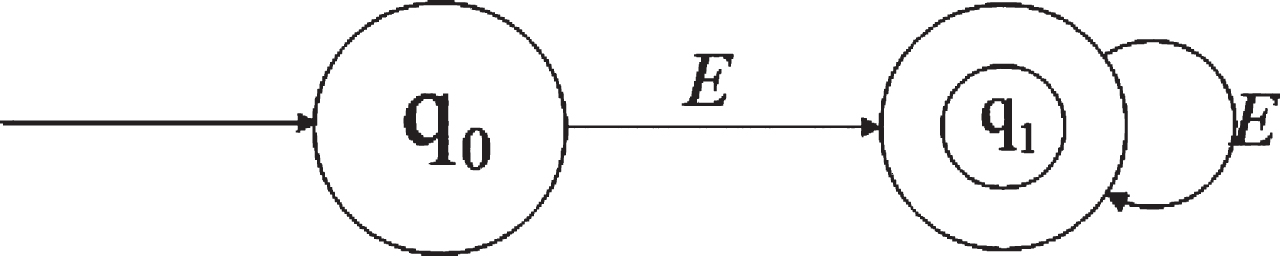
Finite automata A corresponding to Gref (P _safe ).

Given a GPDP M and generalized possibilistic regular safety property P _safe  = {A₀, A₁, … ∈ Σ ^ω ∣ ∀ i ≥ 0, A _i  (E) >0}, Adv is the scheduler defined in M. The solution processes of GPo _max  (s₀ ⊨ P _safe ) and GPo _min  (s₀ ⊨ P _safe ) corresponding to Adv is the maximum scheduler and the minimum scheduler are given.

The product M ⊗ A of a GPDP M and P _safe good prefix Gref (P _safe ) corresponding to a finite automata A is shown in Fig. 5. According to formulas 17 and 18, there B = S × {q₁} = {1, 1, 1} is

Fig. 5

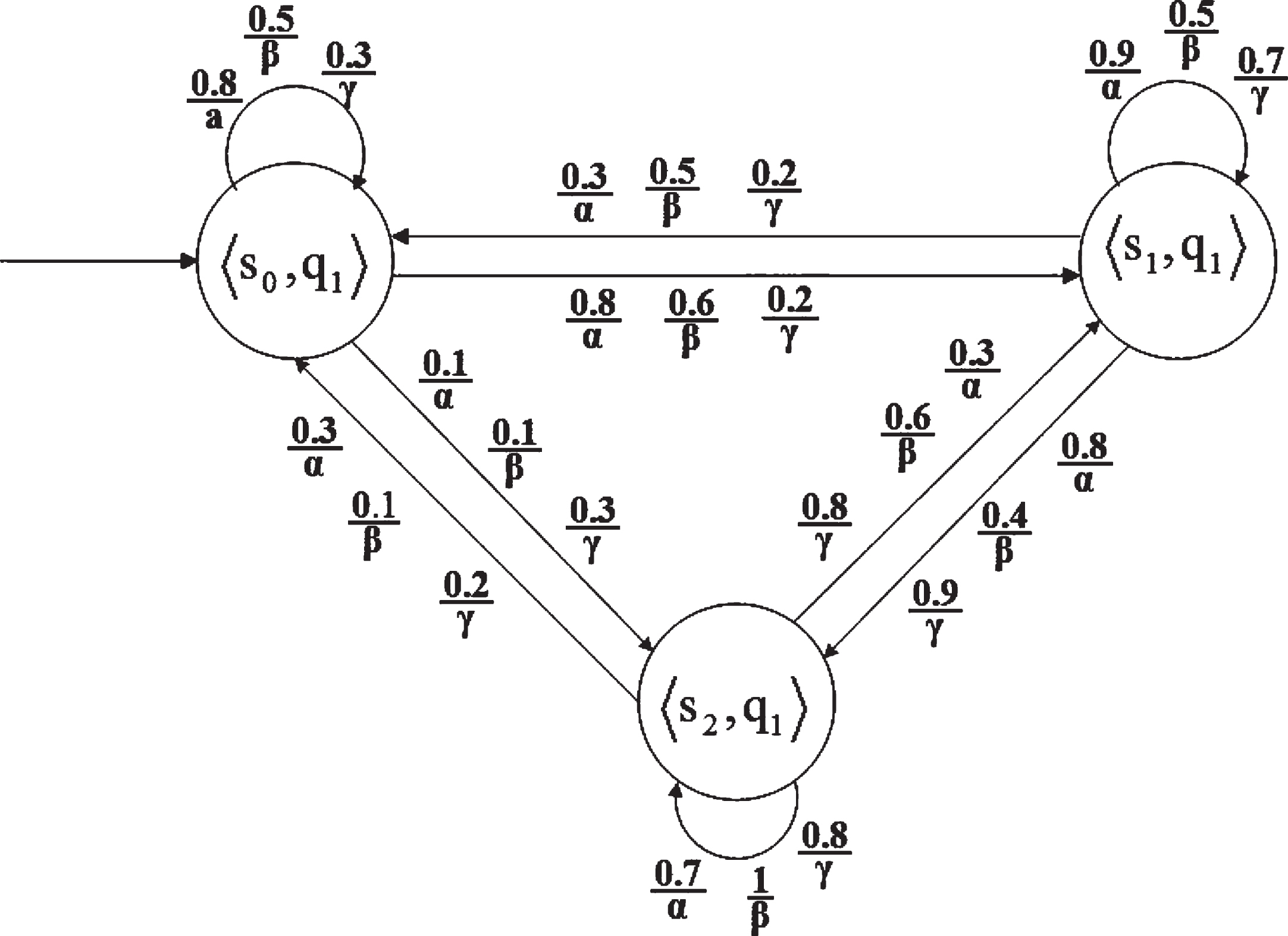
Product GPDPs M ⊗ A.

$\begin{array}{cc}\hfill & f\left(z_1\right)=B\wedge (P_{\mathit{max}}^{*}\circ D_z\circ r_{\mathit{max}})\hfill \\ \hfill & =\left(\begin{array}{c}\hfill 1\hfill \\ \hfill 1\hfill \\ \hfill 1\hfill \end{array}\right)\wedge \hfill \\ \hfill & \left({\left(\begin{array}{ccc}\hfill 0.8\hfill & \hfill 0.8\hfill & \hfill 0.3\hfill \\ \hfill 0.5\hfill & \hfill 0.9\hfill & \hfill 0.9\hfill \\ \hfill 0.3\hfill & \hfill 0.8\hfill & \hfill 1\hfill \\ \hfill \hfill \end{array}\right)}^{*}\circ \left(\begin{array}{ccc}\hfill 1\hfill & \hfill 0\hfill & \hfill 0\hfill \\ \hfill 0\hfill & \hfill 1\hfill & \hfill 0\hfill \\ \hfill 0\hfill & \hfill 0\hfill & \hfill 1\hfill \\ \hfill \hfill \end{array}\right)\circ \left(\begin{array}{c}\hfill 0.8\hfill \\ \hfill 0.9\hfill \\ \hfill 1\hfill \end{array}\right)\right)\hfill \\ \hfill & =\left(\begin{array}{c}\hfill 0.8\hfill \\ \hfill 0.9\hfill \\ \hfill 1\hfill \end{array}\right),\hfill \end{array}$ $\begin{array}{cc}\hfill & f\left(z_2\right)=B\wedge (P_{\mathit{max}}^{*}\circ D_{z_1}\circ r_{\mathit{max}})\hfill \\ \hfill & =\left(\begin{array}{c}\hfill 1\hfill \\ \hfill 1\hfill \\ \hfill 1\hfill \end{array}\right)\wedge \hfill \\ \hfill & \left({\left(\begin{array}{ccc}\hfill 0.8\hfill & \hfill 0.8\hfill & \hfill 0.3\hfill \\ \hfill 0.5\hfill & \hfill 0.9\hfill & \hfill 0.9\hfill \\ \hfill 0.3\hfill & \hfill 0.8\hfill & \hfill 1\hfill \\ \hfill \hfill \end{array}\right)}^{*}\circ \left(\begin{array}{ccc}\hfill 0.8\hfill & \hfill 0\hfill & \hfill 0\hfill \\ \hfill 0\hfill & \hfill 0.9\hfill & \hfill 0\hfill \\ \hfill 0\hfill & \hfill 0\hfill & \hfill 1\hfill \\ \hfill \hfill \end{array}\right)\circ \left(\begin{array}{c}\hfill 0.8\hfill \\ \hfill 0.9\hfill \\ \hfill 1\hfill \end{array}\right)\right)\hfill \\ \hfill & =\left(\begin{array}{c}\hfill 0.8\hfill \\ \hfill 0.9\hfill \\ \hfill 1\hfill \end{array}\right),\hfill \end{array}$

fz₁ = fz₂, Therefore $\begin{array}{cc}\hfill {\mathit{GPo}}_{\mathit{max}}\left(B\right)=\left(\begin{array}{c}\hfill 0.8\hfill \\ \hfill 0.9\hfill \\ \hfill 1\hfill \end{array}\right).& \hfill \end{array}$

Calculated by the same method $\begin{array}{cc}\hfill {\mathit{GPo}}_{\mathit{min}}\left(B\right)=\left(\begin{array}{c}\hfill 0.3\hfill \\ \hfill 0.5\hfill \\ \hfill 0.7\hfill \end{array}\right).& \hfill \end{array}$

GPo _max  (s₀ ⊨ P _safe ) =0.8,GPo _min  (s₀ ⊨ P _safe ) =0.3 are obtained, which shows that the maximum possibility and minimum possibility of generalized possibilistic regular safety property P _safe in GPDPs M are 0.8 and 0.3.

6 Conclusion

In this paper, firstly, we propose GPDPs as the models of nondeterministic and concurrent fuzzy systems. Then, we give fuzzy matrices calculation methods of the maximal possibilities and the minimal possibilities of reachabilities. Finally, we propose a model checking approach to convert the verification of safety property into the analysis of reachabilities. We have given the method of optimization algorithm for reachability. In the future, we will investigate the optimization algorithm for reachability to solve the verification of other properties, such as liveness and fairness in fuzzy systems.

Acknowledgments

The work is partially supported by National Natural Science Foundation of China(Grant No. 61962001), Graduate Innovation Project of North Minzu University(Grant No. YCX22184 and No. YCX22196).

Appendix

Proof. [Proof of Theorem 1]

Since S and Act is finite, given the scheduler Adv, the possibility transition matrix P _Adv is also finite. Obviously, the fuzzy meet operator ∧ does not generate new element,so the set $\left\{\underset{i\ge 0}{\wedge }{P}_{\mathit{Adv}}\right(s_i,{\alpha }_i,s_{i+1})\mid s_i\in S,{\alpha }_i\in \mathit{Act}\}$ is finite.Since S and Act is finite, for any states s ∈ S under consideration of the scheduler Adv, there exits t ∈ S and i < j so that s _i  = s _j  = t.

In this case, P _Adv  (s, α₀, s₁)∧ P _Adv  (s₁, α₁, s₂) ∧ ⋯

= P _Adv  (s, α₀, s₁) ∧ ⋯ ∧ P _Adv  (s_i-1, α_i-1, t) ∧ (P _Adv  (t, α _i , s_i+1)

∧⋯ P _Adv  (s_j-1, α _j , t)) ∧ ⋯

≤P _Adv  (s, α₀, s₁) ∧ ⋯ ∧ P _Adv  (s_i-1, α_i-1, t) ∧ (P _Adv  (t, α _i , s_i+1)

∧ ⋯ ∧ P _Adv  (s_j-1, α _j , t))

$\le P_{\mathit{Adv}}^{+}(s,\mathit{Act}(s),t)\wedge P_{\mathit{Adv}}^{+}(t,\mathit{Act}(t),t)$ .

Hence, $r_{\mathit{Adv}}\left(s\right)\le P_{\mathit{Adv}}^{+}(s,\mathit{Act}(s),t)\wedge P_{\mathit{Adv}}^{+}(t,\mathit{Act}(t),t)$ .

Conversely, for any t ∈ S and schedulers Adv, by the definition of $P_{\mathit{Adv}}^{+}$ , there exists ss₁ ⋯ s _i  = t ∈ S and s_i+1 ⋯ s _j such that

$P_{\mathit{Adv}}^{+}\left(s,t\right)=P_{\mathit{Adv}}(s,s_1)\wedge \cdots \wedge P_{\mathit{Adv}}\left(s_{i-1},t\right)$

$P_{\mathit{Adv}}^{+}\left(t,t\right)=P_{\mathit{Adv}}(t,s_1)\wedge \cdots \wedge P_{\mathit{Adv}}\left(s_j,t\right)$ .

Let π _Adv  = s₀ α₀s₁ α₁ ⋯ s_i-1 α_i-1tα _i  (s_i+1 ⋯ s _j   α _j t)  ^ω,then $P_{\mathit{Adv}}^{+}\left(s,t\right)\wedge P_{\mathit{Adv}}^{+}\left(t,t\right)=P_{\mathit{Adv}}(s,s_1)\wedge P_{\mathit{Adv}}(s_1,s_2)\wedge \cdots .$

Hence, $P_{\mathit{Adv}}^{+}\left(s,t\right)\wedge P_{\mathit{Adv}}^{+}\left(t,t\right)\le r_{\mathit{Adv}}\left(s\right)$ , $\bigvee \{P_{\mathit{Adv}}^{+}\left(s,t\right)\wedge P_{\mathit{Adv}}^{+}\left(t,t\right)\mid t\in S\}\le r_{\mathit{Adv}}\left(s\right).$

Therefore, $r_{\mathit{Adv}}\left(s\right)=\vee \{P_{\mathit{Adv}}^{+}\left(s,t\right)\wedge P_{\mathit{Adv}}^{+}\left(t,t\right)\mid t\in S\}$ .

Proof. [Proof of Theorem 2]

From $\mathit{Cyl}\left(\hat{\pi }\right)=\{\pi \in \mathit{Path}{s}_{\mathit{Adv}}(M)\mid \hat{\pi }\in \mathit{Pref}(\pi \left)\right\}$ , we have Cyl (s₀ α₀s₁ α₁ ⋯ α_n-1s _n ) = ⋃ {π _Adv  ∈ Paths _Adv  (M) ∣ s₀ α₀ ⋯ α_n-1s _n  ∈ Pref (π _Adv )} .

Therefore, GPo  (Cyl (s₀ α₀ ⋯ α_n-1s _n ) )

= ⋁ {GPo (π _Adv ) ∣ s₀ α₀ ⋯ α_n-1s _n  ∈ Pref (π _Adv )}

$=\bigvee \{I\left(s_0\right)\wedge \underset{i\ge 0}{\bigwedge }{P}_{\mathit{Adv}}(s_i,{\alpha }_i,s_{i+1})\mid s_0{\alpha }_0{s}_1\cdots {\alpha }_{n-1}{s}_n\in \mathit{Pref}\left({\pi }_{\mathit{Adv}}\right)\}=\{I\left(s_0\right)\wedge {\bigwedge }_{i=0}^{n-1}{P}_{\mathit{Adv}}(s_i,{\alpha }_i,s_{i+1})\}\wedge \bigwedge \{\underset{j\ge n}{\bigwedge }{P}_{\mathit{Adv}}(s_j,{\alpha }_j,s_{j+1})\}$

$=I\left(s_0\right)\wedge {\bigwedge }_{i=0}^{n-1}{P}_{\mathit{Adv}}\left(s_i,{\alpha }_i,s_{i+1}\right)\}\wedge r_{\mathit{Adv}}(s_n).$

Proof. [Proof of Theorem 3]

GPo _max  (s ⊨ ⋄ B)

= ⋁ _{π∈Paths max (s)}  (GPo _max  (π) ∧ ∥ ⋄ B ∥ (π) )

$=\bigvee ({\bigwedge }_{i=0}^{\infty }{\bigvee }_{{\alpha }_i\in \mathit{Act}}P(s_i,{\alpha }_i,s_{i+1})\wedge {\bigvee }_{j=0}^{\infty }B\left(s_j\right))$

$=\bigvee {\bigvee }_{i=0}^{\infty }(P_{\mathit{max}}(s,s_1)\wedge \dots \wedge P_{\mathit{max}}(s_{i-1},s_i)\wedge B\left(s_i\right))\wedge \bigvee {\bigwedge }_{j=i}^{\infty }{P}_{\mathit{max}}(s_j,s_{j+1})$

$={\bigvee }_{i=0}^{\infty }\bigvee (P_{\mathit{max}}(s,s_1)\wedge \dots \wedge P_{\mathit{max}}(s_{i-1},s_i)\wedge B\left(s_i\right)\wedge r_{\mathit{max}}\left(s_i\right))$

$={\bigvee }_{i=0}^{\infty }(P_{\mathit{max}}^i\circ D_B\circ r_{\mathit{max}})\left(s\right)$

$=\left(\right({\bigvee }_{i=0}^{\infty }{P}_{\mathit{max}}^i)\circ D_B\circ r_{\mathit{max}})\left(s\right)$

$=(P_{\mathit{max}}^{*}\circ D_B\circ r_{\mathit{max}})\left(s\right)$

where P _max is the maximum possibility transition matrix under the max scheduler, Kleene closure of P _max is $P_{\mathit{max}}^{*}$ , D _B is the diagonal matrix diag (B (s)) _s∈S, $r_{\mathit{max}}=P_{\mathit{max}}^{+}\circ D$ , $P_{\mathit{max}}^{+}=P_{\mathit{max}}\vee P_{\mathit{max}}^{*}$ , $D=\left(P_{\mathit{max}}^{+}\right(t,t){)}_{t\in S}$ .

GPo _min  (s ⊨ ⋄ B)

= ⋁ _{π∈Paths min (s)}  (GPo _min  (π) ∧ ∥ ⋄ B ∥ (π) )

$=\bigvee ({\bigwedge }_{i=0}^{\infty }{\bigwedge }_{{\alpha }_i\in \mathit{Act}}P(s_i,{\alpha }_i,s_{i+1})\wedge {\bigvee }_{j=0}^{\infty }B\left(s_j\right))$

$=\bigvee {\bigvee }_{i=0}^{\infty }(P_{\mathit{min}}(s,s_1)\wedge \dots \wedge P_{\mathit{min}}(s_{i-1},s_i)\wedge B\left(s_i\right))\wedge \bigvee {\bigwedge }_{j=i}^{\infty }{P}_{\mathit{min}}(s_j,s_{j+1})$

$={\bigvee }_{i=0}^{\infty }\bigvee (P_{\mathit{min}}(s,s_1)\wedge \dots \wedge P_{\mathit{min}}(s_{i-1},s_i)\wedge B\left(s_i\right)\wedge r_{\mathit{min}}\left(s_i\right))$

$={\bigvee }_{i=0}^{\infty }(P_{\mathit{min}}^i\circ D_B\circ r_{\mathit{min}})\left(s\right)$

$=\left(\right({\bigvee }_{i=0}^{\infty }{P}_{\mathit{min}}^i)\circ D_B\circ r_{\mathit{min}})\left(s\right)$

$=(P_{\mathit{min}}^{*}\circ D_B\circ r_{\mathit{min}})\left(s\right),$

where P _min is the minimum possibility transition matrix under the min scheduler.

Proof. [Proof of Theorem 5]

GPo _max  (s ⊨ C ⊔ ^≤nB) = ⋁ _{π∈Paths max (s)}  (GPo _max  (π) ∧ ∥ C ⊔ ^≤nB ∥ (π) )

= ⋁  (⋁  _{α0∈Act(s0)}P (s₀, α₀, s₁) ∧ ⋁  _{α1∈Act(s1)}P (s₁, α₁, s₂)

$\wedge \dots \wedge ({\bigvee }_{j\ge 0}^{n}B\left(s_j\right)\wedge {\bigwedge }_{i\le j}C\left(s_i\right)))$

$=\bigvee (P_{\mathit{max}}(s_0,s_1)\wedge P_{\mathit{max}}(s_1,s_2)\wedge \dots \wedge ({\bigvee }_{j\ge 0}^{n}B\left(s_j\right)\wedge {\bigwedge }_{i\le j}C\left(s_i\right)))$

$=(B\left(s_0\right)\wedge r_{\mathit{max}}\left(s_0\right))\vee ({\bigvee }_{j\ge 0}^{n}C\left(s_j\right)\wedge {\bigwedge }_{i\le j}{P}_{\mathit{max}}(s_{i-1},s_i)\wedge C\left(s_i\right)\wedge P_{\mathit{max}}(s_{j-1},s_j)\wedge B\left(s_j\right)\wedge r_{\mathit{max}}\left(s_j\right))$

$=\left({\bigvee }_{i=0}^n\right(D_C\circ P_{\mathit{max}}{)}_i\circ D_B\circ r_{\mathit{max}}\left)\right(s).$

GPo _min  (s ⊨ C ⊔ ^≤nB)

= ⋁ _{π∈Paths min (s)}  (GPo _min  (π) ∧ ∥ C ⊔ ^≤nB ∥ (π) )

$=\bigvee ({\bigwedge }_{{\alpha }_0\in \mathit{Act}\left(s_0\right)}P(s_0,{\alpha }_0,s_1)\wedge {\bigwedge }_{{\alpha }_1\in \mathit{Act}\left(s_1\right)}P(s_1,{\alpha }_1,s_2)\wedge \dots \wedge ({\bigvee }_{j\ge 0}^{n}B\left(s_j\right)\wedge {\bigwedge }_{i\le j}C\left(s_i\right)))$

$=\bigvee (P_{\mathit{min}}(s_0,s_1)\wedge P_{\mathit{min}}(s_1,s_2)\wedge \dots \wedge ({\bigvee }_{j\ge 0}^{n}B\left(s_j\right)\wedge {\bigwedge }_{i\le j}C\left(s_i\right)))$

$=(B\left(s_0\right)\wedge r_{\mathit{min}}\left(s_0\right))\vee ({\bigvee }_{j\ge 0}^{n}C\left(s_j\right)\wedge {\bigwedge }_{i\le j}{P}_{\mathit{min}}(s_{i-1},s_i)\wedge C\left(s_i\right)\wedge P_{\mathit{min}}(s_{j-1},s_j)\wedge B\left(s_j\right)\wedge r_{\mathit{min}}\left(s_j\right))$

$=\left({\bigvee }_{i=0}^n\right(D_C\circ P_{\mathit{min}}{)}_i\circ D_B\circ r_{\mathit{min}}\left)\right(s).$

Proof. [Proof of Theorem 6]

GPo _Adv  (s ⊨  ⋄ B) = ⋁ _{π∈Paths Adv (s)}  (GPo (π) ∧ ∥  ⋄ B ∥ (π) ). Let π = s₀ α₀s₁ α₁ … ∈ Paths _Adv  (s₀), inf (π) denotes the set of states that occur infinitely many times on the path π, then ∥  ⋄ B ∥ (π) ≤ ⋁ _t∈inf(π)B (t). Furthermore, for any t ∈ inf (π), π ⊨  ⋄ t, we can get GPo _Adv  (π) ≤ GPo _Adv  ({π ∈ Paths _fin  (s) ∣ π ⊨  ⋄ t} ) , thus GPo _Adv  (π) ∧ ∥  ⋄ B ∥ (π) ≤ ⋁ _t∈inf(π) > (B (t) ∧ GPo _Adv  (s ⊨  ⋄ t) ) ≤ ⋁ _t∈S  (B (t) ∧ GPo _Adv  (s ⊨  ⋄ t) ) . Therefore, GPo _Adv  (s ⊨  ⋄ B) ≤ ⋁ _t∈S  (B (t) ∧ GPo _Adv  (s ⊨  ⋄ t) ) .

Conversely, for any state t ∈ S, and any path π ∈ Paths _Adv  (s) that satisfies the event  ⋄ t,we have B (s) ≤ ∥  ⋄ B ∥ (π). It follows that ⋁_t∈S  (B (t) ∧ GPo _Adv  (s ⊨  ⋄ t) ) ≤ ⋁ _t∈S  (B (t) ∧ GPo _Adv  (s ⊨  ⋄ t) ), therefore, ⋁_t∈S  (B (t) ∧ GPo _Adv  (s ⊨  ⋄ t) ) ≤ GPo _Adv  (s ⊨  ⋄ B).

In conclusion, GPo _Adv  (s⊨  ⋄ B) = ⋁ _t∈SB (t) ∧

GPo _Adv  (s ⊨  ⋄ t) .

We can get the method to calculate GPo _Adv  (s ⊨  ⋄ t) from these results, that is ${\mathit{GPo}}_{\mathit{Adv}}(s\models \diamond t)=P_{\mathit{Adv}}^{+}(s,t)\wedge P_{\mathit{Adv}}^{+}(t,t)$ . Then we obtain ${\mathit{GPo}}_{\mathit{Adv}}(s\models \diamond B)={\bigvee }_{t\in S}B\left(t\right)\wedge P_{\mathit{Adv}}^{+}(s,t)\wedge P_{\mathit{Adv}}^{+}(t,t).$

When the Adv is the maximum possibility scheduler and the minimum possibility scheduler, we can get Theorem 6.

Proof. [Proof of Theorem 7]

GPo _max  (s ⊨ ⋄  B)

= ⋁ _{π∈Paths max (s)}  (GPo _max  (π) ∧ ∥ ⋄  B ∥ (π) )

$=\bigvee ({\mathit{GPo}}_{\mathit{max}}\left(\pi \right)\wedge {\bigvee }_{i=0}^{\infty }{\bigwedge }_{j=i}^{\infty }B\left(s_j\right))$

$=\bigvee {\bigvee }_{i=0}^{\infty }({\bigvee }_{{\alpha }_0\in \mathit{Act}}P(s,{\alpha }_0,s_1)\wedge {\bigvee }_{{\alpha }_1\in \mathit{Act}}P(s_1,{\alpha }_1,s_2)\wedge \dots \wedge {\bigvee }_{{\alpha }_{i-1}\in \mathit{Act}}P(s_{i-1},{\alpha }_{i-1},s_i)\wedge B\left(s_i\right)\wedge {\bigvee }_{{\alpha }_i\in \mathit{Act}}P(s_i,{\alpha }_i,s_{i+1})$

∧B (s_i+1) ∧ ⋁  _αi+1∈ActP (s_i+1, α_i+1, s_i+2) ∧ B (s_i+2) ∧ … )

$=\bigvee {\bigvee }_{i=0}^{\infty }(P_{\mathit{max}}(s,s_1)\wedge P_{\mathit{max}}(s_1,s_2)\wedge \dots \wedge P_{\mathit{max}}\left(s_{i-1}{s}_i\right)\wedge B\left(s_i\right)\wedge P_{\mathit{max}}(s_i,s_{i+1})\wedge B\left(s_{i+1}\right)\wedge P_{\mathit{max}}(s_{i+1},s_{i+2})\wedge$

B (s_i+2) ∧ … )

$=\bigvee {\bigvee }_{i=0}^{\infty }(P_{\mathit{max}}(s,s_1)\wedge P_{\mathit{max}}(s_1,s_2)\wedge \dots \wedge P_{\mathit{max}}\left(s_{i-1}{s}_i\right)$

∧ (D _max  ∘ P _max ) (s _i , s_i+1) ∧ (D _max  ∘ P _max ) (s_i+1, s_i+2)

∧ … )

$=\bigvee {\bigvee }_{i=0}^{\infty }(P_{\mathit{max}}(s,s_1)\wedge P_{\mathit{max}}(s_1,s_2)\wedge \dots \wedge P_{\mathit{max}}\left(s_{i-1}{s}_i\right)$

∧r_{D B ∘P max}  (s _i ) )

$={\bigvee }_{i=0}^{\infty }({\bigvee }_{s_i\in S}(P_{\mathit{max}}(s,s_1)\wedge P_{\mathit{max}}(s_1,s_2)\wedge \dots )\wedge$

P _max  (s_i-1s _i ) ∧ r_{D B ∘P max}  (s _i ) )

$={\bigvee }_{i=0}^{\infty }(P_{\mathit{max}}^i\circ r_{D_B\circ P_{\mathit{max}}}\left(s\right))=\left({\bigvee }_{i=0}^{\infty }{P}_{\mathit{max}}^i\right)\circ r_{D_B\circ P_{\mathit{max}}}\left(s\right)$

$=P_{\mathit{max}}^{*}\circ r_{D_B\circ P_{\mathit{max}}}\left(s\right),$

GPo _min  (s ⊨ ⋄  B)

= ⋁ _{π∈Paths min (s)}  (GPo _min  (π) ∧ ∥ ⋄  B ∥ (π) )

$=\bigvee ({\mathit{GPo}}_{\mathit{min}}\left(\pi \right)\wedge {\bigvee }_{i=0}^{\infty }{\bigwedge }_{j=i}^{\infty }B\left(s_j\right))$

$=\bigvee {\bigvee }_{i=0}^{\infty }({\bigwedge }_{{\alpha }_0\in \mathit{Act}}P(s,{\alpha }_0,s_1)\wedge {\bigwedge }_{{\alpha }_1\in \mathit{Act}}P(s_1,{\alpha }_1,s_2)\wedge \dots \wedge {\bigwedge }_{{\alpha }_{i-1}\in \mathit{Act}}P(s_{i-1},{\alpha }_{i-1},s_i)\wedge B\left(s_i\right)\wedge {\bigwedge }_{{\alpha }_i\in \mathit{Act}}P(s_i,{\alpha }_i,s_{i+1})\wedge B\left(s_{i+1}\right)\wedge {\bigwedge }_{{\alpha }_{i+1}\in \mathit{Act}}P(s_{i+1},{\alpha }_{i+1},s_{i+2})\wedge B\left(s_{i+2}\right)\wedge \dots )$

$=\bigvee {\bigvee }_{i=0}^{\infty }(P_{\mathit{min}}(s,s_1)\wedge P_{\mathit{min}}(s_1,s_2)\wedge \dots \wedge P_{\mathit{min}}\left(s_{i-1}{s}_i\right)\wedge B\left(s_i\right)\wedge P_{\mathit{min}}(s_i,s_{i+1})\wedge B\left(s_{i+1}\right)\wedge P_{\mathit{min}}(s_{i+1},s_{i+2})\wedge B\left(s_{i+2}\right)\wedge \dots )$

$=\bigvee {\bigvee }_{i=0}^{\infty }(P_{\mathit{min}}(s,s_1)\wedge P_{\mathit{min}}(s_1,s_2)\wedge \dots \wedge P_{\mathit{min}}\left(s_{i-1}{s}_i\right)\wedge (D_{\mathit{min}}\circ P_{\mathit{min}})(s_i,s_{i+1})\wedge (D_{\mathit{min}}\circ P_{\mathit{min}})(s_{i+1},s_{i+2})\wedge \dots )$

$=\bigvee {\bigvee }_{i=0}^{\infty }(P_{\mathit{min}}(s,s_1)\wedge P_{\mathit{min}}(s_1,s_2)\wedge \dots \wedge P_{\mathit{min}}\left(s_{i-1}{s}_i\right)\wedge r_{D_B\circ P_{\mathit{min}}}\left(s_i\right))={\bigvee }_{i=0}^{\infty }({\bigvee }_{s_i\in S}(P_{\mathit{min}}(s,s_1)\wedge P_{\mathit{min}}(s_1,s_2)\wedge \dots )\wedge P_{\mathit{min}}\left(s_{i-1}{s}_i\right)\wedge r_{D_B\circ P_{\mathit{min}}}\left(s_i\right))$

$={\bigvee }_{i=0}^{\infty }(P_{\mathit{min}}^i\circ r_{D_B\circ P_{\mathit{min}}}\left(s\right))=\left({\bigvee }_{i=0}^{\infty }{P}_{\mathit{min}}^i\right)\circ r_{D_B\circ P_{\mathit{min}}}\left(s\right)=P_{\mathit{min}}^{*}\circ r_{D_B\circ P_{\mathit{min}}}\left(s\right).$

Proof. [Proof of Theorem 8]

${\mathit{GPo}}_{\mathit{Adv}}^M(s\models P_{\mathit{safe}})$

= ⋁ _{π∈Paths Adv (s)}  (GPo _Adv  (π) ∧ P _safe  (Trace _Adv  (π)) )

= ⋁  (GPo _Adv  (π) ∧ ⋀ _j≥0  {L (A) (θ) ∣ θ ∈ Pref (Trace _Adv  (π)) } )

= ⋁  (GPo _Adv  (π) ∧ ⋀ _j≥0  {F (q _j ) ∣ q _j δ^* (q₀, L (s) L (s₁) … L (s _j )) } ) ⋁  (GPo _Adv  (π) ∧ ⋀ _i≥0F (q _i ) ) .

For π = sα₀s₁ α₁ … ∈ Paths _Adv  (s), we define the run sequence q₀q₁q₂… of the deterministic fuzzy finite automata by q_i+1 = δ (q _i , L (s _i )). Vice versa, for the same run sequence q₀q₁q₂… of the deterministic fuzzy finite automata, we have

${\mathit{GPo}}_{\mathit{Adv}}^{M\otimes A}(<a,q_s>\models B)$

= ⋁ _{π⁺∈Paths Adv (<s,q s >)}  (GPo _Adv  (π⁺) ∧ ⋀ _i≥0B (π⁺ [i]) )

= ⋁ _{π∈Paths Adv (s)}  (GPo _Adv  (π) ∧ ⋀ _i≥0F (q _i ) ) ,