Sage Journals: Discover world-class research

Abstract

A recent three-dimensional (3D) model that revisited earlier theoretical work for longitudinal electromagnetic stirring in the continuous casting of steel blooms is analyzed further to explore how the bloom width interacts with the pole pitch of the stirrer to affect the magnetic flux density. Whereas the first work indicated the presence of a boundary layer in the steel near the interface with the stirrer, with all three components of the magnetic flux density vector being coupled to each other, in the analysis presented here we find that the component along the direction of the travelling wave decouples from those in the other two directions and can even be determined analytically in the form of a series solution. Moreover, it is found that the remaining two components can be found via a two-dimensional computation, but that it is not possible in general to determine these components without taking into account the surrounding air. The validity of the asymptotically reduced model solution is confirmed by comparing it with the results of 3D numerical computations. Moreover, the asymptotic approach provides a way to compute the time-averaged Lorentz force components that requires two orders of magnitude less computational time than the fully 3D approach.

Keywords

Asymptotic analysis continuous casting electromagnetic stirring

1. Introduction

Electromagnetic stirring (EMS) is the process by which a high level of stirring efficiency can be achieved through interaction between the magnetic field from a static induction coil and an electrically conducting metal bath. It has long been used in the steel industry as a way to affect the flow of molten metal during the continuous casting process, both in the ladle and during the solidification in the casting machine itself [1–3]; more recently, EMS has also been used in the magnesium and aluminium industries [4,5]. At the same time, mathematical modelling has been used for the purposes of understanding exactly what effect EMS has on the metal flow.

A series of papers by Schwerdtfeger and co-workers [6–11], originally written in the context of the continuous casting of steel, explored both experimentally and theoretically the effect of EMS in the round-billet, rectangular-bloom and slab configurations that are typical for this process; these have formed the basis of modelling in this area and are even cited until the present day [12–20]. The theoretical models developed consist of Maxwell’s equations for the induced magnetic flux density and the Navier Stokes equations for the velocity field of the molten metal; in principle, these equations are two-way coupled, since the alternating magnetic field gives rise to a Lorentz force which drives the velocity field, which can in turn affect the magnetic field. Typically, however, the magnetic Reynolds number is small enough that the velocity field does not affect the spatial and temporal distribution of the magnetic field, implying only one-way coupling. A further often-invoked simplification is that the frequency of the magnetic field is typically large enough to allow the use of the time-averaged value of the Lorentz force as input to the Navier Stokes equations, rather than having to solve for the velocity and magnetic fields simultaneously.

However, on revisiting the problem of rotary EMS in round-billet continuous casting, Vynnycky [21] recently found that the method used originally in [6,11] to determine the components of the Lorentz force did not lead to a unique solution; this was because the normal component of the induced magnetic flux density, rather than the tangential ones, had been prescribed as the boundary condition. Thereafter, Nick and Vynnycky [22] revisited the models for the corresponding problem for longitudinal stirring in rectangular blooms, originally considered in [7–10]; in addition to the issue of the appropriate boundary condition at the interface between the stirrer and the steel were the conditions to be taken at the interfaces between the steel and the surrounding air. Moreover, through nondimensionalization, it was found that the key dimensionless parameter in the model, Δ, was the product of the the wave vector and the width of the bloom, and that this parameter was comparatively large (approximately 13) in the models in [7–10]. Interestingly, previous literature had not remarked on the significance of this quantity and its cause is different to the more well-documented skin effect [23], which is related to the frequency of the magnetic field. Furthermore, it was possible to carry out an asymptotic analysis of the problem which identified the structure of the field; this essentially consisted of a boundary layer having a dimensionless width of order of 1∕Δ near the surface of the stirrer in which all magnetic flux density vector components decreased rapidly to zero. A follow-on question is then what happens when Δ is not large, as might occur if a smaller bloom and a larger pole pitch is used. Thus, the purpose of this manuscript is to consider, still in the low magnetic Reynolds number limit as in [22], the corresponding analysis when Δ is small; although this can no doubt be done solely numerically using commercially available software, the benefit of the analysis given here is that elucidates more clearly the dependencies of the magnetic flux density, the current density and the Lorentz force components on the applied boundary conditions and key dimensionless parameters. In addition, this gives a way to determine these quantities at a fraction of the computational cost that full 3D simulations require.

The structure of the paper is as follows. In Sections 2 and 3, we recap the mathematical formulation of the problem and the nondimensionalization of the governing equations, respectively. The new analysis, in terms of the asymptotically small parameter Δ, is given in Section 4, whilst Section 5 outlines the numerical method used to solve the fully three-dimensional (3D) and reduced two-dimensional (2D) time-dependent problems. The results are presented in Section 6, and conclusions are drawn in Section 7.

2. Model formulation

2.1. Governing equations

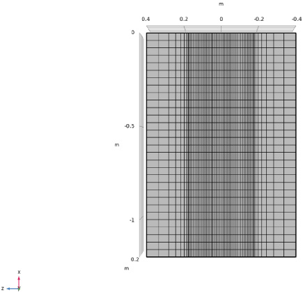
We consider, as depicted in Fig. 1, a linear travelling stirrer that is situated at y = 0, −h∕2 ≤ z ≤ h∕2, −l ≤ x ≤ 0, operating on a molten steel region whose cross-section is given by 0 ≤ y ≤ b, −h∕2 ≤ z ≤ h∕2, as shown in Fig. 2; the steel is surrounded by air on the other three sides. As explained in [22], this is a simplification of the actual situation in a continuous casting process, but we have nevertheless retained enough to carry out a meaningful analysis with respect to determining the characteristics of the magnetic flux density.

Fig. 1.

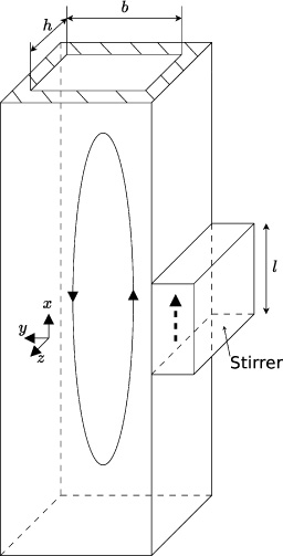
Schematic for the longitudinal stirring of blooms and billets. A travelling wave is passed along the casting (x) direction.

Fig. 2.

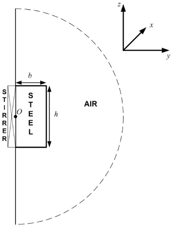
Cross-section in the y-z plane of Fig. 1, showing the stirrer, steel and air. O denotes the origin of the coordinates.

We consider the solution of Maxwell’s equations in the magnetohydrodynamic (MHD) approximation, which consist of:

the magnetic field constraint, $\begin{eqnarray}\displaystyle {\nabla}\cdot \mathbf{B}=0, & & \displaystyle\end{eqnarray}$ (1) where B is the magnetic flux density vector;

Ampère’s law, $\begin{eqnarray}\displaystyle \mathbf{J}+{\displaystyle \frac{\partial \mathbf{D}}{\partial t}}={\nabla}\times \mathbf{H}, & & \displaystyle\end{eqnarray}$ (2) where J is the electrical current density vector, H is the magnetic field strength, which is related to B via the magnetic permeability, 𝜂, by B = 𝜂H, and D is the displacement current, although we shall neglect it in what follows;

Faraday’s law, $\begin{eqnarray}\displaystyle {\nabla}\times \mathbf{E}=-{\displaystyle \frac{\partial \mathbf{B}}{\partial t}}, & & \displaystyle\end{eqnarray}$ (3) where E is the electric field and t is time;

Ohm’s law, $\begin{eqnarray}\displaystyle \mathbf{J}={\sigma}(\mathbf{E}+\boldsymbol{v}\times \mathbf{B}), & & \displaystyle\end{eqnarray}$ (4) where v is the velocity vector, which we will simply set to zero, and σ is the electrical conductivity of the medium under consideration, which we take to be constant in both steel and air.

Manipulating (2)–(4), we obtain $\begin{eqnarray}\displaystyle {\sigma}{\eta}{\displaystyle \frac{\partial \mathbf{B}}{\partial t}}={\nabla}^{2}\mathbf{B}; & & \displaystyle\end{eqnarray}$ (5) note, however, that this must still be solved together with Eq. (1). Thus, with B _x, B _y and B _z as x-, y- and z-components, respectively, of B, we have $\begin{eqnarray}\displaystyle \text{} & \text{} & \displaystyle {\displaystyle \frac{\partial B_{x}}{\partial x}}+{\displaystyle \frac{\partial B_{y}}{\partial y}}+{\displaystyle \frac{\partial B_{z}}{\partial z}}=0,\end{eqnarray}$ (6) $\begin{eqnarray}\displaystyle \text{} & \text{} & \displaystyle {\sigma}{\eta}{\displaystyle \frac{\partial B_{x}}{\partial t}}={\displaystyle \frac{\partial ^{2}B_{x}}{\partial x^{2}}}+{\displaystyle \frac{\partial ^{2}B_{x}}{\partial y^{2}}}+{\displaystyle \frac{\partial ^{2}B_{x}}{\partial z^{2}}},\end{eqnarray}$ (7) $\begin{eqnarray}\displaystyle \text{} & \text{} & \displaystyle {\sigma}{\eta}{\displaystyle \frac{\partial B_{y}}{\partial t}}={\displaystyle \frac{\partial ^{2}B_{y}}{\partial x^{2}}}+{\displaystyle \frac{\partial ^{2}B_{y}}{\partial y^{2}}}+{\displaystyle \frac{\partial ^{2}B_{y}}{\partial z^{2}}},\end{eqnarray}$ (8) $\begin{eqnarray}\displaystyle \text{} & \text{} & \displaystyle {\sigma}{\eta}{\displaystyle \frac{\partial B_{z}}{\partial t}}={\displaystyle \frac{\partial ^{2}B_{z}}{\partial x^{2}}}+{\displaystyle \frac{\partial ^{2}B_{z}}{\partial y^{2}}}+{\displaystyle \frac{\partial ^{2}B_{z}}{\partial z^{2}}}.\end{eqnarray}$ (9)

Once B _x, B _y and B _z have been computed, the quantities of principal interest are the components of the Lorentz force, F _x, F _y and F _z, which are given by $\begin{eqnarray}\displaystyle F_{x}=J_{y}B_{z}-J_{z}B_{y},\quad F_{y}=J_{z}B_{x}-J_{x}B_{z},\quad F_{z}=J_{x}B_{y}-J_{y}B_{x}, & & \displaystyle\end{eqnarray}$ (10) where (J _x, J _y, J _z) are the components of J and are given by $\begin{eqnarray}\displaystyle \left(\begin{array}{@{}c@{}}J_{x}\\ J_{y}\\ J_{z}\end{array}\right)={\displaystyle \frac{1}{{\eta}}}\left(\begin{array}{@{}c@{}}\displaystyle {\displaystyle \frac{\partial B_{z}}{\partial y}}-{\displaystyle \frac{\partial B_{y}}{\partial z}}\\[12.0pt] \displaystyle {\displaystyle \frac{\partial B_{x}}{\partial z}}-{\displaystyle \frac{\partial B_{z}}{\partial x}}\\[12.0pt] \displaystyle {\displaystyle \frac{\partial B_{y}}{\partial x}}-{\displaystyle \frac{\partial B_{x}}{\partial y}}\end{array}\right). & & \displaystyle\end{eqnarray}$ (11) Finally, F _x, F _y and F _z are used to calculate the time-averaged Lorentz force components - $\overline{F}_x$ , $\overline{F}_y$ and $\overline{F}_z$ - via $\begin{eqnarray}\displaystyle \bar{F}_{k}={\displaystyle \frac{1}{2{\pi}/{\omega}}}\displaystyle \int _{0}^{2{\pi}/{\omega}}F_{k}\text{d}t^{\prime },\quad k=x,y,z, & & \displaystyle\end{eqnarray}$ (12) with the integrals in (12) being taken with respect to time over one period of oscillation, 2π∕ω, and with ω as the angular frequency of the current.

2.2. Boundary and interfacial conditions

At y = 0, as discussed previously [22], we prescribe the tangential components of B; thus, $\begin{eqnarray}\displaystyle \text{} & \text{} & \displaystyle B_{x}=\left\{\begin{array}{@{}ll@{}}{\alpha}(z)\cos ({\omega}t-{\lambda}x) & \text{for }|z|\leq h/2\\ 0 & \text{for }|z|>h/2,\end{array}\right.\end{eqnarray}$ (13) $\begin{eqnarray}\displaystyle \text{} & \text{} & \displaystyle B_{z}=\left\{\begin{array}{@{}ll@{}}{\beta}(z)\cos ({\omega}t-{\lambda}x) & \text{for }|z|\leq h/2\\ 0 & \text{for }|z|>h/2,\end{array}\right.\end{eqnarray}$ (14) where 𝜆 is the wave vector given by 𝜆 = π∕p, with p as the pole pitch, i.e. the distance from north to south pole in the inductor. For orientation, Fig. 3 shows the common time-dependent part of Eqs (13) and (14), cos(ωt −𝜆x), as a function of x for four different values of t during one period of oscillation. For this figure, we have made use of the parameters shown in Table 1 in the following way: ω is related to the current frequency, f, by ω =2πf; on the other hand, since 𝜆b turns out to be an important dimensionless parameter in the problem, we have used the value of b in Table 1 and plotted profiles for the cases where 𝜆 = 0.01∕b and 0.1∕b. Note here that the plotted function is sinusoidal in nature, although this may not be apparent from these plots because of the comparatively small values of 𝜆, relative to the stirrer length, l.

Fig. 3.

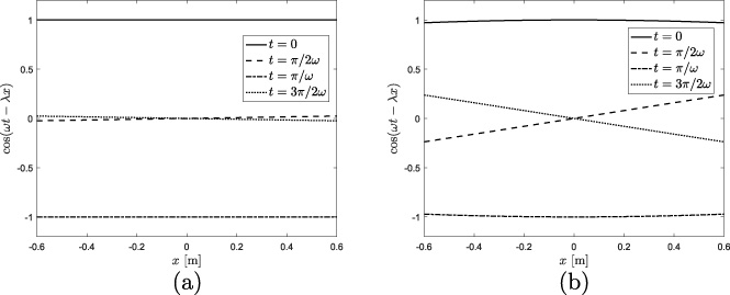
cos(ωt −𝜆x) vs. x for: (a) 𝜆 = 0.01∕b; (b) 𝜆 = 0.1∕b.

Table 1

Model parameters

Parameter	Symbol	Value
Steel width	b	0.25 m
Characteristic magnetic flux density	B ₀	0.02 T
Current frequency	f	50 Hz
Steel breadth	h	0.35 m
Stirrer length	l	1.2 m
Air magnetic permeability	𝜂_a	1.2566 ×10⁻⁶ Vs A⁻¹ m⁻¹
Steel magnetic permeability	𝜂_s	1.2566 ×10⁻⁶ Vs A⁻¹ m⁻¹
Air electrical conductivity	σ_a	3 ×10⁻¹⁵ −8 ×10⁻¹⁵ A V⁻¹ m⁻¹
Steel electrical conductivity	σ_s	7.14 ×10⁵ A V⁻¹ m⁻¹

For the steel-air interfaces at y = b, |z| ≤ h∕2 and |z| = h∕2, 0 ≤ y ≤ b, we apply the conventional electromagnetic interface conditions between two media. These are the continuity of the tangential components of the magnetic field strength, the continuity of the normal component of the magnetic flux density and the continuity of the tangential components of the electric field; these are written, respectively, as $\begin{eqnarray}\displaystyle \text{} & \text{} & \displaystyle \left[{\displaystyle \frac{\mathbf{B}\cdot \mathbf{t}}{{\eta}}}\right]_{-}^{+}=0,\end{eqnarray}$ (15) $\begin{eqnarray}\displaystyle \text{} & \text{} & \displaystyle [\mathbf{B}\cdot \mathbf{n}]_{-}^{+}=0,\end{eqnarray}$ (16) $\begin{eqnarray}\displaystyle \text{} & \text{} & \displaystyle [\mathbf{E}\cdot \mathbf{t}]_{-}^{+}=0,\end{eqnarray}$ (17) where t and n are the unit tangential and normal vectors, respectively, at these interfaces. In (15)–(17), $[\text{ }]_{-}^{+}$ is taken to mean the difference in the value of a function in the air (+) and in the steel (−).

In the air far from the steel, we should also expect the magnetic flux density to vanish, so we take $\begin{eqnarray}\displaystyle \mathbf{B}\rightarrow 0\quad \text{as }r\rightarrow \infty , & & \displaystyle\end{eqnarray}$ (18) where $r=\sqrt{x^{2}+y^{2}+z^{2}}$ .

3. Nondimensionalization

We nondimensionalize the equations by setting $\begin{eqnarray}\displaystyle X={\displaystyle \frac{x}{l}},\quad Y={\displaystyle \frac{y}{b}},\quad Z={\displaystyle \frac{z}{b}},\quad {\tau}={\displaystyle \frac{{\omega}t}{2{\pi}}}, & & \displaystyle\end{eqnarray}$ (19) and for k = x, y, z and K = X, Y, Z, $\begin{eqnarray}\displaystyle B_{K}={\displaystyle \frac{B_{k}}{B_{0}}},\quad E_{K}={\displaystyle \frac{E_{k}}{B_{0}/{\sigma}_{s}{\eta}_{s}b}},\quad J_{K}={\displaystyle \frac{J_{k}}{B_{0}/{\eta}_{s}b}},\quad F_{K}={\displaystyle \frac{F_{k}}{B_{0}^{2}/{\eta}_{s}b}}, & & \displaystyle \nonumber\end{eqnarray}$ where B ₀ is the characteristic magnetic flux density, and 𝜂_s and σ_s are the steel magnetic permeability and electrical conductivity, respectively. Equations (6)–(9) give $\begin{eqnarray}\displaystyle \text{} & \text{} & \displaystyle {\delta}{\displaystyle \frac{\partial B_{X}}{\partial X}}+{\displaystyle \frac{\partial B_{Y}}{\partial Y}}+{\displaystyle \frac{\partial B_{Z}}{\partial Z}}=0,\end{eqnarray}$ (20) $\begin{eqnarray}\displaystyle \text{} & \text{} & \displaystyle {\Omega}{\displaystyle \frac{\partial B_{X}}{\partial {\tau}}}={\delta}^{2}{\displaystyle \frac{\partial ^{2}B_{X}}{\partial X^{2}}}+{\displaystyle \frac{\partial ^{2}B_{X}}{\partial Y^{2}}}+{\displaystyle \frac{\partial ^{2}B_{X}}{\partial Z^{2}}},\end{eqnarray}$ (21) $\begin{eqnarray}\displaystyle \text{} & \text{} & \displaystyle {\Omega}{\displaystyle \frac{\partial B_{Y}}{\partial {\tau}}}={\delta}^{2}{\displaystyle \frac{\partial ^{2}B_{Y}}{\partial X^{2}}}+{\displaystyle \frac{\partial ^{2}B_{Y}}{\partial Y^{2}}}+{\displaystyle \frac{\partial ^{2}B_{Y}}{\partial Z^{2}}},\end{eqnarray}$ (22) $\begin{eqnarray}\displaystyle \text{} & \text{} & \displaystyle {\Omega}{\displaystyle \frac{\partial B_{Z}}{\partial {\tau}}}={\delta}^{2}{\displaystyle \frac{\partial ^{2}B_{Z}}{\partial X^{2}}}+{\displaystyle \frac{\partial ^{2}B_{Z}}{\partial Y^{2}}}+{\displaystyle \frac{\partial ^{2}B_{Z}}{\partial Z^{2}}},\end{eqnarray}$ (23) where 𝛺 = fσ𝜂b ² and δ = b∕l. However, note that the values for 𝛺 for steel and air, 𝛺_s and 𝛺_a respectively, are different; from the data in Table 1, it is evident that 𝛺_s ≫ 𝛺_a. Also, from (11), (10) and (12), respectively, we have $\begin{eqnarray}\displaystyle \text{} & \text{} & \displaystyle \left(\begin{array}{@{}c@{}}J_{X}\\ J_{Y}\\ J_{Z}\end{array}\right)=\left(\begin{array}{@{}c@{}}\displaystyle {\displaystyle \frac{\partial B_{Z}}{\partial Y}}-{\displaystyle \frac{\partial B_{Y}}{\partial Z}}\\[6.0pt] \displaystyle \frac{\partial B_{X}}{\partial Z}-{\delta}{\displaystyle \frac{\partial B_{Z}}{\partial X}}\\[6.0pt] \displaystyle {\delta}\frac{\partial B_{Y}}{\partial X}-{\displaystyle \frac{\partial B_{X}}{\partial Y}}\end{array}\right),\end{eqnarray}$ (24) $\begin{eqnarray}\displaystyle \text{} & \text{} & \displaystyle F_{X}=J_{Y}B_{Z}-J_{Z}B_{Y},\quad F_{Y}=J_{Z}B_{X}-J_{X}B_{Z},\quad F_{Z}=J_{X}B_{Y}-J_{Y}B_{X},\end{eqnarray}$ (25) $\begin{eqnarray}\displaystyle \text{} & \text{} & \displaystyle \bar{F}_{K}=\displaystyle \int _{0}^{1}F_{K}\text{d}t^{\prime },\quad K=X,Y,Z.\end{eqnarray}$ (26)

The boundary conditions (13)–(18) are then: at Y = 0, $\begin{eqnarray}\displaystyle \text{} & \text{} & \displaystyle B_{X}=\left\{\begin{array}{@{}ll@{}}\bar{{\alpha}}(Z)\cos (2{\pi}{\tau}-{\Lambda}X) & \text{for }|Z|\leq H/2\\ 0 & \text{for }|Z|>H/2,\end{array}\right.\end{eqnarray}$ (27) $\begin{eqnarray}\displaystyle \text{} & \text{} & \displaystyle B_{Z}=\left\{\begin{array}{@{}ll@{}}\bar{{\beta}}(Z)\cos (2{\pi}{\tau}-{\Lambda}X) & \text{for }|Z|\leq H/2\\ 0 & \text{for }|Z|>H/2,\end{array}\right.\end{eqnarray}$ (28) where $\begin{eqnarray}\displaystyle \bar{{\alpha}}={\displaystyle \frac{{\alpha}}{[{\alpha}]}},\quad \bar{{\beta}}={\displaystyle \frac{{\beta}}{[{\beta}]}},\quad {\Lambda}={\lambda}l,\quad H={\displaystyle \frac{h}{b}}, & & \displaystyle \nonumber\end{eqnarray}$ with [𝛼] and [𝛽] denoting, respectively, the scales for 𝛼 and 𝛽; at Y = 1, |Z| ≤ H∕2 and |Z| = H∕2,0 ≤ Y ≤ 1, $\begin{eqnarray}\displaystyle \text{} & \text{} & \displaystyle \left[{\displaystyle \frac{\mathbf{B}\cdot \mathbf{t}}{{\eta}}}\right]_{-}^{+}=0,\end{eqnarray}$ (29) $\begin{eqnarray}\displaystyle \text{} & \text{} & \displaystyle [\mathbf{B}\cdot \mathbf{n}]_{-}^{+}=0,\end{eqnarray}$ (30) $\begin{eqnarray}\displaystyle \text{} & \text{} & \displaystyle [\mathbf{E}\cdot \mathbf{t}]_{-}^{+}=0;\end{eqnarray}$ (31) as R →∞, where $R=\sqrt{X^{2}+Y^{2}+Z^{2}}$ , $\begin{eqnarray}\displaystyle \mathbf{B}\rightarrow 0. & & \displaystyle\end{eqnarray}$ (32)

4. Analysis

As in [22], equation (20) and the boundary conditions in (27) imply that the solutions for B _X, B _Y and B _Z will have the form $\begin{eqnarray}\displaystyle B_{X},B_{Y},B_{Z}\sim \left\{\begin{array}{@{}l@{}}\cos (2{\pi}{\tau}-{\Lambda}X)\\ \sin (2{\pi}{\tau}-{\Lambda}X).\end{array}\right. & & \displaystyle \nonumber\end{eqnarray}$ Thus, we will first set $\begin{eqnarray}\displaystyle \left.\begin{array}{@{}c@{}}B_{k}=\mathfrak{Re}({\mathcal{B}}_{k}(Y,Z)e^{\text{i}(2{\pi}{\tau}-{\Lambda}X)}),\\[4.0pt] E_{k}=\mathfrak{Re}({\mathcal{E}}_{k}(Y,Z)e^{\text{i}(2{\pi}{\tau}-{\Lambda}X)}),\end{array}\right\}\quad k=X,Y,Z, & & \displaystyle \nonumber\end{eqnarray}$ with i = √ − 1 and $\mathfrak{Re}$ denoting the real part of a complex number. Equations (20)–(23) become $\begin{eqnarray}\displaystyle \text{} & \text{} & \displaystyle -{\Delta}\text{i}{\mathcal{B}}_{X}+{\displaystyle \frac{\partial {\mathcal{B}}_{Y}}{\partial Y}}+{\displaystyle \frac{\partial {\mathcal{B}}_{Z}}{\partial Z}}=0,\end{eqnarray}$ (33) $\begin{eqnarray}\displaystyle \text{} & \text{} & \displaystyle (2{\pi}{\Omega}_{i}\text{i}+{\Delta}^{2}){\mathcal{B}}_{X}={\displaystyle \frac{\partial ^{2}{\mathcal{B}}_{X}}{\partial Y^{2}}}+{\displaystyle \frac{\partial ^{2}{\mathcal{B}}_{X}}{\partial Z^{2}}},\end{eqnarray}$ (34) $\begin{eqnarray}\displaystyle \text{} & \text{} & \displaystyle (2{\pi}{\Omega}_{i}\text{i}+{\Delta}^{2}){\mathcal{B}}_{Y}={\displaystyle \frac{\partial ^{2}{\mathcal{B}}_{Y}}{\partial Y^{2}}}+{\displaystyle \frac{\partial ^{2}{\mathcal{B}}_{Y}}{\partial Z^{2}}},\end{eqnarray}$ (35) $\begin{eqnarray}\displaystyle \text{} & \text{} & \displaystyle (2{\pi}{\Omega}_{i}\text{i}+{\Delta}^{2}){\mathcal{B}}_{Z}={\displaystyle \frac{\partial ^{2}{\mathcal{B}}_{Z}}{\partial Y^{2}}}+{\displaystyle \frac{\partial ^{2}{\mathcal{B}}_{Z}}{\partial Z^{2}}},\end{eqnarray}$ (36) where Δ = 𝜆b and i = a, s. In terms of ${\mathcal{B}}_{X},{\mathcal{B}}_{Y}$ and ${\mathcal{B}}_{Z}$ , the boundary conditions are now: at Y = 0, $\begin{eqnarray}\displaystyle \text{} & \text{} & \displaystyle {\mathcal{B}}_{X}=\left\{\begin{array}{@{}ll@{}}\bar{{\alpha}}(Z) & \quad \text{for }|Z|\leq H/2\\ 0 & \quad \text{for }|Z|>H/2,\end{array}\right.\end{eqnarray}$ (37) $\begin{eqnarray}\displaystyle \text{} & \text{} & \displaystyle {\mathcal{B}}_{Z}=\left\{\begin{array}{@{}ll@{}}\bar{{\beta}}(Z) & \quad \text{for }|Z|\leq H/2\\ 0 & \quad \text{for }|Z|>H/2;\end{array}\right.\end{eqnarray}$ (38) at Y = 1, |Z| ≤ H∕2, $\begin{eqnarray}\displaystyle \text{} & \text{} & \displaystyle \left[{\displaystyle \frac{{\mathcal{B}}_{X}}{{\eta}}}\right]_{-}^{+}=0,\end{eqnarray}$ (39) $\begin{eqnarray}\displaystyle \text{} & \text{} & \displaystyle [{\mathcal{B}}_{Y}]_{-}^{+}=0,\end{eqnarray}$ (40) $\begin{eqnarray}\displaystyle \text{} & \text{} & \displaystyle \left[{\displaystyle \frac{{\mathcal{B}}_{Z}}{{\eta}}}\right]_{-}^{+}=0,\end{eqnarray}$ (41) $\begin{eqnarray}\displaystyle \text{} & \text{} & \displaystyle \left[{\displaystyle \frac{1}{{\sigma}{\eta}}}\left({\displaystyle \frac{\partial {\mathcal{B}}_{Z}}{\partial Y}}-{\displaystyle \frac{\partial {\mathcal{B}}_{Y}}{\partial Z}}\right)\right]_{-}^{+}=0,\end{eqnarray}$ (42) $\begin{eqnarray}\displaystyle \text{} & \text{} & \displaystyle \left[{\displaystyle \frac{1}{{\sigma}{\eta}}}\left(-\text{i}{\Delta}{\mathcal{B}}_{Z}-{\displaystyle \frac{\partial {\mathcal{B}}_{X}}{\partial Z}}\right)\right]_{-}^{+}=0;\end{eqnarray}$ (43) at |Z| = H∕2, 0 ≤ Y ≤ 1, $\begin{eqnarray}\displaystyle \text{} & \text{} & \displaystyle \left[{\displaystyle \frac{{\mathcal{B}}_{X}}{{\eta}}}\right]_{-}^{+}=0,\end{eqnarray}$ (44) $\begin{eqnarray}\displaystyle \text{} & \text{} & \displaystyle \left[{\displaystyle \frac{{\mathcal{B}}_{Y}}{{\eta}}}\right]_{-}^{+}=0,\end{eqnarray}$ (45) $\begin{eqnarray}\displaystyle \text{} & \text{} & \displaystyle [{\mathcal{B}}_{Z}]_{-}^{+}=0,\end{eqnarray}$ (46) $\begin{eqnarray}\displaystyle \text{} & \text{} & \displaystyle \left[{\displaystyle \frac{1}{{\sigma}{\eta}}}\left({\displaystyle \frac{\partial {\mathcal{B}}_{Z}}{\partial Y}}-{\displaystyle \frac{\partial {\mathcal{B}}_{Y}}{\partial Z}}\right)\right]_{-}^{+}=0,\end{eqnarray}$ (47) $\begin{eqnarray}\displaystyle \text{} & \text{} & \displaystyle \left[{\displaystyle \frac{1}{{\sigma}{\eta}}}\left(-\text{i}{\Delta}{\mathcal{B}}_{Y}-{\displaystyle \frac{\partial {\mathcal{B}}_{X}}{\partial Y}}\right)\right]_{-}^{+}=0;\end{eqnarray}$ (48) and, as R →∞, $\begin{eqnarray}\displaystyle {\mathcal{B}}_{X},{\mathcal{B}}_{Y},{\mathcal{B}}_{Z}\rightarrow 0. & & \displaystyle\end{eqnarray}$ (49)

Our earlier work [22] considered the case Δ ≫ 1, and we identified a boundary layer of thickness 1∕Δ near the surface of the stirrer. This time, we consider the other extreme when Δ ≪ 1, whilst treating the parameters 𝛺_a and 𝛺_s as being of O (1). Note also that if we had had 𝛺_s ≫ 1, this would have led to the skin-effect case; however, 𝛺_s ≫ 1 still does not lead to the Δ ≫ 1 case considered in [22], since there is no term in 𝛺_s in (33). This further emphasizes the fact that the problem treated in [22] was not that of the classical skin-effect type.

We first determine the solutions for B _X, B _Y and B _Z; thereafter, these are used to constitute expressions for J _X, J _Y, J _Z, F _X, F _Y and F _Z.

4.1. B _X, B _Y, B _Z

In what follows, we assume that $\bar{{\alpha}},\bar{{\beta}}\neq 0$ and that $\bar{{\alpha}},\bar{{\beta}}\sim O(1)$ ; the analysis proceeds slightly differently if $\bar{{\alpha}}\neq 0,\bar{{\beta}}=∼0$ or $\bar{{\alpha}}=∼0,\bar{{\beta}}\neq 0$ , and these cases are considered in appendices A and B, respectively.

We set $\begin{eqnarray}\displaystyle \left.\begin{array}{@{}l@{}}B_{k}=B_{k}^{(0)}+{\Delta}B_{k}^{(1)}+O({\Delta}^{2})\\[4.0pt] {\mathcal{B}}_{k}={\mathcal{B}}_{k}^{(0)}+{\Delta}{\mathcal{B}}_{k}^{(1)}+O({\Delta}^{2})\end{array}\right\},\quad k=X,Y,Z, & & \displaystyle\end{eqnarray}$ (50) which is motivated by the appearance of the terms in Δ in Eqs (33), (43) and (48). We have, at O (Δ⁰), $\begin{eqnarray}\displaystyle \text{} & \text{} & \displaystyle {\displaystyle \frac{\partial {\mathcal{B}}_{Y}^{(0)}}{\partial Y}}+{\displaystyle \frac{\partial {\mathcal{B}}_{Z}^{(0)}}{\partial Z}}=0,\end{eqnarray}$ (51) $\begin{eqnarray}\displaystyle \text{} & \text{} & \displaystyle 2{\pi}{\Omega}_{i}\text{i}{\mathcal{B}}_{X}^{(0)}={\displaystyle \frac{\partial ^{2}{\mathcal{B}}_{X}^{(0)}}{\partial Y^{2}}}+{\displaystyle \frac{\partial ^{2}{\mathcal{B}}_{X}^{(0)}}{\partial Z^{2}}},\end{eqnarray}$ (52) $\begin{eqnarray}\displaystyle \text{} & \text{} & \displaystyle 2{\pi}{\Omega}_{i}\text{i}{\mathcal{B}}_{Y}^{(0)}={\displaystyle \frac{\partial ^{2}{\mathcal{B}}_{Y}^{(0)}}{\partial Y^{2}}}+{\displaystyle \frac{\partial ^{2}{\mathcal{B}}_{Y}^{(0)}}{\partial Z^{2}}},\end{eqnarray}$ (53) $\begin{eqnarray}\displaystyle \text{} & \text{} & \displaystyle 2{\pi}{\Omega}_{i}\text{i}{\mathcal{B}}_{Z}^{(0)}={\displaystyle \frac{\partial ^{2}{\mathcal{B}}_{Z}^{(0)}}{\partial Y^{2}}}+{\displaystyle \frac{\partial ^{2}{\mathcal{B}}_{Z}^{(0)}}{\partial Z^{2}}},\end{eqnarray}$ (54) subject to: at Y = 0, $\begin{eqnarray}\displaystyle \text{} & \text{} & \displaystyle {\mathcal{B}}_{X}^{(0)}=\left\{\begin{array}{@{}ll@{}}\bar{{\alpha}}(Z) & \quad \text{for }|Z|\leq H/2\\ 0 & \quad \text{for }|Z|>H/2,\end{array}\right.\end{eqnarray}$ (55) $\begin{eqnarray}\displaystyle \text{} & \text{} & \displaystyle {\mathcal{B}}_{Z}^{(0)}=\left\{\begin{array}{@{}ll@{}}\bar{{\beta}}(Z) & \quad \text{for }|Z|\leq H/2\\ 0 & \quad \text{for }|Z|>H/2;\end{array}\right.\end{eqnarray}$ (56) at Y = 1, |Z| ≤ H∕2, $\begin{eqnarray}\displaystyle \text{} & \text{} & \displaystyle \left[{\displaystyle \frac{{\mathcal{B}}_{X}^{(0)}}{{\eta}}}\right]_{-}^{+}=0,\end{eqnarray}$ (57) $\begin{eqnarray}\displaystyle \text{} & \text{} & \displaystyle [{\mathcal{B}}_{Y}^{(0)}]_{-}^{+}=0,\end{eqnarray}$ (58) $\begin{eqnarray}\displaystyle \text{} & \text{} & \displaystyle \left[{\displaystyle \frac{{\mathcal{B}}_{Z}^{(0)}}{{\eta}}}\right]_{-}^{+}=0,\end{eqnarray}$ (59) $\begin{eqnarray}\displaystyle \text{} & \text{} & \displaystyle \left[{\displaystyle \frac{1}{{\sigma}{\eta}}}\left({\displaystyle \frac{\partial {\mathcal{B}}_{Z}^{(0)}}{\partial Y}}-{\displaystyle \frac{\partial {\mathcal{B}}_{Y}^{(0)}}{\partial Z}}\right)\right]_{-}^{+}=0,\end{eqnarray}$ (60) $\begin{eqnarray}\displaystyle \text{} & \text{} & \displaystyle \left[{\displaystyle \frac{1}{{\sigma}{\eta}}}{\displaystyle \frac{\partial {\mathcal{B}}_{X}^{(0)}}{\partial Z}}\right]_{-}^{+}=0;\end{eqnarray}$ (61) at |Z| = H∕2, 0 ≤ Y ≤ 1, $\begin{eqnarray}\displaystyle \text{} & \text{} & \displaystyle \left[{\displaystyle \frac{{\mathcal{B}}_{X}^{(0)}}{{\eta}}}\right]_{-}^{+}=0,\end{eqnarray}$ (62) $\begin{eqnarray}\displaystyle \text{} & \text{} & \displaystyle \left[{\displaystyle \frac{{\mathcal{B}}_{Y}^{(0)}}{{\eta}}}\right]_{-}^{+}=0,\end{eqnarray}$ (63) $\begin{eqnarray}\displaystyle \text{} & \text{} & \displaystyle [{\mathcal{B}}_{Z}^{(0)}]_{-}^{+}=0,\end{eqnarray}$ (64) $\begin{eqnarray}\displaystyle \text{} & \text{} & \displaystyle \left[{\displaystyle \frac{1}{{\sigma}{\eta}}}\left({\displaystyle \frac{\partial {\mathcal{B}}_{Z}^{(0)}}{\partial Y}}-{\displaystyle \frac{\partial {\mathcal{B}}_{Y}^{(0)}}{\partial Z}}\right)\right]_{-}^{+}=0,\end{eqnarray}$ (65) $\begin{eqnarray}\displaystyle \text{} & \text{} & \displaystyle \left[{\displaystyle \frac{1}{{\sigma}{\eta}}}{\displaystyle \frac{\partial {\mathcal{B}}_{X}^{(0)}}{\partial Y}}\right]_{-}^{+}=0;\end{eqnarray}$ (66) as R → ∞, $\begin{eqnarray}\displaystyle {\mathcal{B}}_{X}^{(0)},{\mathcal{B}}_{Y}^{(0)},{\mathcal{B}}_{Z}^{(0)}\rightarrow 0. & & \displaystyle\end{eqnarray}$ (67)

We can now see that, in contrast to the case when Δ ≫ 1, the equations for ${\mathcal{B}}_{Y}^{(0)}$ and ${\mathcal{B}}_{Z}^{(0)}$ , i.e. (51), (53) and (54), subject to (56), (58)–(60), (63)–(65) and the last two conditions in (67), decouple from those for ${\mathcal{B}}_{X}^{(0)}$ , i.e. (52), subject to (55), (57), (61), (62), (66) and the first condition in (67), and can therefore be solved separately.

4.1.1.

{\mathcal{B}}_{X}^{(0)}

Further simplification is now possible in view of the fact that σ_a∕σ_s ≪ 1, 𝜂_a∕𝜂_s = 1, as seen from Table 1. Therefore, equations (61) and (66) reduce to $\begin{eqnarray}\displaystyle \text{} & \text{} & \displaystyle \left({\displaystyle \frac{\partial {\mathcal{B}}_{X}^{(0)}}{\partial Z}}\right)_{+}\approx 0,\nonumber\\ \displaystyle \text{} & \text{} & \displaystyle \left({\displaystyle \frac{\partial {\mathcal{B}}_{X}^{(0)}}{\partial Y}}\right)_{+}\approx 0,\nonumber\end{eqnarray}$ respectively; this means that the solution in the air has effectively decoupled from that in the steel. Moreover, since ${\mathcal{B}}_{X}^{(0)}$ satisfies a homogeneous partial differential equation (PDE) and is subject to homogeneous boundary conditions, it is clear that ${\mathcal{B}}_{X}^{(0)}\equiv 0$ in the air; hence, (57) and (62) then both give $\begin{eqnarray}\displaystyle ({\mathcal{B}}_{X}^{(0)})_{-}=0, & & \displaystyle \nonumber\end{eqnarray}$ which then leads to the following problem for ${\mathcal{B}}_{X}^{(0)}$ , which needs only to be solved in the steel: equation (52), subject to $\begin{eqnarray}\displaystyle \text{} & \text{} & \displaystyle {\mathcal{B}}_{X}^{(0)}=\bar{{\alpha}}(Z)\quad \text{for }Y=0,|Z|\leq H/2,\end{eqnarray}$ (68) $\begin{eqnarray}\displaystyle \text{} & \text{} & \displaystyle {\mathcal{B}}_{X}^{(0)}=0\quad \text{for }Y=1,|Z|\leq H/2,\end{eqnarray}$ (69) $\begin{eqnarray}\displaystyle \text{} & \text{} & \displaystyle {\mathcal{B}}_{X}^{(0)}=0\quad \text{for }|Z|=H/2,0<Y<1.\end{eqnarray}$ (70)

It is now possible to construct an analytical series solution for ${\mathcal{B}}_{X}^{(0)}$ for 0 ≤ Y ≤ 1, |Z| ≤ H∕2. Trying a solution of the form $\begin{eqnarray}\displaystyle {\mathcal{B}}_{X}^{(0)}\sim g_{n}(Y)\sin {\displaystyle \frac{n{\pi}}{H}}\left(Z-{\displaystyle \frac{H}{2}}\right), & & \displaystyle\end{eqnarray}$ (71) since this satisfies (70), we have $\begin{eqnarray}\displaystyle g_{n}^{\prime \prime }-{\mu}_{n}^{2}g_{n}=0, & & \displaystyle\end{eqnarray}$ (72) where $\begin{eqnarray}\displaystyle {\mu}_{n}^{2}={\displaystyle \frac{n^{2}{\pi}^{2}}{H^{2}}}+2{\pi}{\Omega}_{s}\text{i}, & & \displaystyle\end{eqnarray}$ (73) which will give $\begin{eqnarray}\displaystyle g_{n}=A_{n}\sinh ({\mu}_{n}(1-Y))+B_{n}\cosh ({\mu}_{n}(1-Y)), & & \displaystyle\end{eqnarray}$ (74) where A _n and B _n are constants to be determined. Since we require g _n(1) = 0 from (69), where the prime denotes differentiation with respect to Y , we must have B _n = 0. To determine A _n, we will have, on using (68), $\begin{eqnarray}\displaystyle \bar{{\alpha}}(Z)=\mathop{\sum }_{n=1}^{\infty }A_{n}\sinh {\mu}_{n}\sin {\displaystyle \frac{n{\pi}}{H}}\left(Z-{\displaystyle \frac{H}{2}}\right). & & \displaystyle\end{eqnarray}$ (75) Multiplying both of sides of (75) by $\sin \frac{m{\pi}}{H}(Z-\frac{H}{2})$ , m = 1,2, …, and integrating from Z = −H∕2 to Z = H∕2, we obtain $\begin{eqnarray}\displaystyle A_{n}={\displaystyle \frac{2I_{n}}{H\sinh {\mu}_{n}}},\quad n=1,2,\ldots , & & \displaystyle\end{eqnarray}$ (76) where $\begin{eqnarray}\displaystyle I_{n}=\displaystyle \int _{-H/2}^{H/2}\bar{{\alpha}}(Z^{\prime })\sin {\displaystyle \frac{n{\pi}}{H}}\left(Z^{\prime }-{\displaystyle \frac{H}{2}}\right)\text{d}Z^{\prime },\quad n=1,2,\ldots , & & \displaystyle\end{eqnarray}$ (77) leading to $\begin{eqnarray}\displaystyle {\mathcal{B}}_{X}^{(0)}=\displaystyle \mathop{\sum }_{n=1}^{\infty }A_{n}\sinh ({\mu}_{n}(1-Y))\sin {\displaystyle \frac{n{\pi}}{H}}\left(Z-{\displaystyle \frac{H}{2}}\right) & & \displaystyle\end{eqnarray}$ (78) as the solution. From this, it is evident that $\begin{eqnarray}\displaystyle B_{X}^{(0)}=\mathfrak{Re}\left(e^{\text{i}(2{\pi}{\tau}-{\Lambda}X)}\displaystyle \mathop{\sum }_{n=1}^{\infty }A_{n}\sinh ({\mu}_{n}(1-Y))\sin {\displaystyle \frac{n{\pi}}{H}}\left(Z-{\displaystyle \frac{H}{2}}\right)\right). & & \displaystyle\end{eqnarray}$ (79)

4.1.2.

{\mathcal{B}}_{Y}^{(0)}

and

{\mathcal{B}}_{Z}^{(0)}

As regards ${\mathcal{B}}_{Y}^{(0)}$ and ${\mathcal{B}}_{Z}^{(0)}$ , it is convenient to consider a formulation in terms of a magnetic vector potential, A = (A (Y, Z), 0, 0), such that $\begin{eqnarray}\displaystyle {\mathcal{B}}_{Y}^{(0)}={\displaystyle \frac{\partial A}{\partial Z}},\quad {\mathcal{B}}_{Z}^{(0)}=-{\displaystyle \frac{\partial A}{\partial Y}}, & & \displaystyle\end{eqnarray}$ (80) i.e. (0, B_Y ⁽⁰⁾, B_Z ⁽⁰⁾) = 𝛻 × A. Equations (53) and (54) give, respectively, $\begin{eqnarray}\displaystyle \text{} & \text{} & \displaystyle {\displaystyle \frac{\partial }{\partial Z}}\left(2{\pi}{\Omega}_{i}\text{i}A-{\displaystyle \frac{\partial ^{2}A}{\partial Y^{2}}}-{\displaystyle \frac{\partial ^{2}A}{\partial Z^{2}}}\right)=0,\end{eqnarray}$ (81) $\begin{eqnarray}\displaystyle \text{} & \text{} & \displaystyle {\displaystyle \frac{\partial }{\partial Y}}\left(2{\pi}{\Omega}_{i}\text{i}A-{\displaystyle \frac{\partial ^{2}A}{\partial Y^{2}}}-{\displaystyle \frac{\partial ^{2}A}{\partial Y^{2}}}\right)=0,\end{eqnarray}$ (82) leading, on integrating with respect to Z and Y respectively, to $\begin{eqnarray}\displaystyle \text{} & \text{} & \displaystyle 2{\pi}{\Omega}_{i}\text{i}A={\displaystyle \frac{\partial ^{2}A}{\partial Y^{2}}}+{\displaystyle \frac{\partial ^{2}A}{\partial Z^{2}}}+{\gamma}_{1}(Y),\end{eqnarray}$ (83) $\begin{eqnarray}\displaystyle \text{} & \text{} & \displaystyle 2{\pi}{\Omega}_{i}\text{i}A={\displaystyle \frac{\partial ^{2}A}{\partial Y^{2}}}+{\displaystyle \frac{\partial ^{2}A}{\partial Z^{2}}}+{\gamma}_{2}(Z),\end{eqnarray}$ (84) where 𝛾₁ and 𝛾₂ are functions to be determined; however, since Y and Z are independent variables, clearly 𝛾₁ and 𝛾₂ can only be constants, with 𝛾₁ = 𝛾₂(= 𝛾). We can write $A_{i}=\bar{A}_{i}+\frac{{\gamma}}{2{\pi}{\Omega}_{i}\text{i}}$ , so that (83) and (84) both give $\begin{eqnarray}\displaystyle 2{\pi}{\Omega}_{i}\text{i}\bar{A}={\displaystyle \frac{\partial ^{2}\bar{A}}{\partial Y^{2}}}+{\displaystyle \frac{\partial ^{2}\bar{A}}{\partial Z^{2}}}. & & \displaystyle\end{eqnarray}$ (85)

For the boundary conditions, we have, in terms of $\bar{A}$ : at Y = 0, $\begin{eqnarray}\displaystyle {\displaystyle \frac{\partial \bar{A}}{\partial Y}}=\left\{\begin{array}{@{}ll@{}}-\bar{{\beta}}(Z) & \quad \text{for }|Z|\leq H/2\\ 0 & \quad \text{for }|Z|>H/2;\end{array}\right. & & \displaystyle\end{eqnarray}$ (86) at Y = 1, |Z| ≤ H∕2, $\begin{eqnarray}\displaystyle \text{} & \text{} & \displaystyle \left[{\displaystyle \frac{\partial \bar{A}}{\partial Z}}\right]_{-}^{+}=0,\end{eqnarray}$ (87) $\begin{eqnarray}\displaystyle \text{} & \text{} & \displaystyle \left[{\displaystyle \frac{1}{{\eta}}}{\displaystyle \frac{\partial \bar{A}}{\partial Y}}\right]_{-}^{+}=0,\end{eqnarray}$ (88) $\begin{eqnarray}\displaystyle \text{} & \text{} & \displaystyle \left[{\displaystyle \frac{1}{{\sigma}{\eta}}}\left({\displaystyle \frac{\partial ^{2}\bar{A}}{\partial Y^{2}}}+{\displaystyle \frac{\partial ^{2}\bar{A}}{\partial Z^{2}}}\right)\right]_{-}^{+}=0;\end{eqnarray}$ (89) at |Z| = H∕2, 0 ≤ Y ≤ 1, $\begin{eqnarray}\displaystyle \text{} & \text{} & \displaystyle \left[{\displaystyle \frac{1}{{\eta}}}{\displaystyle \frac{\partial \bar{A}}{\partial Z}}\right]_{-}^{+}=0,\end{eqnarray}$ (90) $\begin{eqnarray}\displaystyle \text{} & \text{} & \displaystyle \left[{\displaystyle \frac{\partial \bar{A}}{\partial Y}}\right]_{-}^{+}=0,\end{eqnarray}$ (91) $\begin{eqnarray}\displaystyle \text{} & \text{} & \displaystyle \left[{\displaystyle \frac{1}{{\sigma}{\eta}}}\left({\displaystyle \frac{\partial ^{2}\bar{A}}{\partial Y^{2}}}+{\displaystyle \frac{\partial ^{2}\bar{A}}{\partial Z^{2}}}\right)\right]_{-}^{+}=0;\end{eqnarray}$ (92) as R →∞, $\begin{eqnarray}\displaystyle {\displaystyle \frac{\partial \bar{A}}{\partial Y}},{\displaystyle \frac{\partial \bar{A}}{\partial Z}}\rightarrow 0. & & \displaystyle\end{eqnarray}$ (93)

Using (85), we find that (89) and (92) give, at Y = 1, |Z| ≤ H∕2 and |Z| = H∕2, 0 ≤ Y ≤ 1, $\begin{eqnarray}\displaystyle [\bar{A}]_{-}^{+}=0, & & \displaystyle\end{eqnarray}$ (94) which will in turn mean that (87) and (91) are automatically satisfied. At this stage, the equations that remain to be solved are (85), subject to (88), (90), (93) and (94), and we can note that, in general, it is not possible to determine the magnetic field for 0 ≤ Y ≤ 1, |Z| ≤ H∕2 without considering the region outside it.

4.2. J _X, J _Y, J _Z, F _X, F _Y, F _X

Next, with the expansions $\begin{eqnarray}\displaystyle \left.\begin{array}{@{}l@{}}J_{k}=J_{k}^{(0)}+{\Delta}J_{k}^{(1)}+\ldots \\ F_{k}=F_{k}^{(0)}+{\Delta}F_{k}^{(1)}+\ldots \\ \bar{F}_{k}=\bar{F}_{k}^{(0)}+{\Delta}\bar{F}_{k}^{(1)}+\ldots \end{array}\right\},\quad k=X,Y,Z, & & \displaystyle\end{eqnarray}$ (95) we have $\begin{eqnarray}\displaystyle \left(\begin{array}{@{}c@{}}J_{X}^{(0)}\\[5.0pt] J_{Y}^{(0)}\\[5.0pt] J_{Z}^{(0)}\end{array}\right)=\left(\begin{array}{@{}c@{}}\displaystyle {\displaystyle \frac{\partial B_{Z}^{(0)}}{\partial Y}}-{\displaystyle \frac{\partial B_{Y}^{(0)}}{\partial Z}}\\[7.0pt] \displaystyle {\displaystyle \frac{\partial B_{X}^{(0)}}{\partial Z}}\\[7.0pt] \displaystyle -{\displaystyle \frac{\partial B_{X}^{(0)}}{\partial Y}}\end{array}\right), & & \displaystyle\end{eqnarray}$ (96) and the Lorentz force at leading order in Δ is given by $\begin{eqnarray}\displaystyle \left(\begin{array}{@{}c@{}}F_{X}^{(0)}\\[5.0pt] F_{Y}^{(0)}\\[5.0pt] F_{Z}^{(0)}\end{array}\right)=\left(\begin{array}{@{}c@{}}J_{Y}^{(0)}B_{Z}^{(0)}-J_{Z}^{(0)}B_{Y}^{(0)}\\[4.0pt] J_{Z}^{(0)}B_{X}^{(0)}-J_{X}^{(0)}B_{Z}^{(0)}\\[4.0pt] J_{X}^{(0)}B_{Y}^{(0)}-J_{Y}^{(0)}B_{X}^{(0)}\end{array}\right); & & \displaystyle\end{eqnarray}$ (97) then, the leading order time-averaged Lorentz force, $\bar{\mathbf{F}}^{(0)}=(\bar{F}_{X}^{(0)},\bar{F}_{Y}^{(0)},\bar{F}_{Z}^{(0)})$ , is given by $\begin{eqnarray}\displaystyle \bar{\mathbf{F}}^{(0)}={\displaystyle \frac{1}{2}}(\mathfrak{Re}({\mathcal{J}}^{(0)})\times \mathfrak{Re}({\mathcal{B}}^{(0)})+\mathfrak{Im}({\mathcal{J}}^{(0)})\times \mathfrak{Im}({\mathcal{B}}^{(0)})), & & \displaystyle\end{eqnarray}$ (98) where $\begin{eqnarray}\displaystyle {\mathcal{J}}^{(0)}={\nabla}\times {\mathcal{B}}^{(0)}, & & \displaystyle\end{eqnarray}$ (99) with ${\mathcal{B}}^{(0)}=({\mathcal{B}}_{X}^{(0)},{\mathcal{B}}_{Y}^{(0)},{\mathcal{B}}_{Z}^{(0)})$ .

5. Numerical solution

5.1. 3D computations

In order to verify the correctness of the asymptotic analysis, equations (6)–(9), subject to (13)–(18), were also solved numerically. For this, the Magnetic Fields module of the finite-element software Comsol Multiphysics was used, as in [22]. Second-order Lagrangian quadrilateral elements were employed on a mesh having approximately 55000 elements, corresponding to around 1.3 million degrees of freedom. As regards the size of the computational domain, its outer edge was taken to be a half-cylinder with a radius of 0.4 m and a height of 1.2 m. The geometry and the mesh are shown in Figs 4–6. Note that the mesh is somewhat different to that used in [22], since there is no need to refine the mesh near y = 0, as there is no boundary layer for the values of Δ used; on the other hand, the magnetic flux density in the steel does not decay rapidly to zero away from the stirrer, meaning that a more or less uniform mesh is necessary throughout the steel region.

Fig. 4.

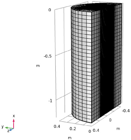
Geometry and mesh used for three-dimensional computations.

Fig. 5.

Mesh used for three-dimensional computations, adjacent to the stirrer face at y = 0.

Fig. 6.

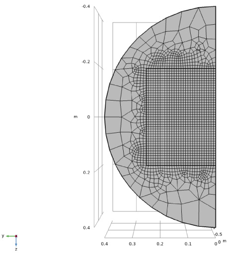
A cross-section in the y-z plane of the mesh used for three-dimensional computations.

Adaptive time-stepping was used for the numerical integration, and the convergence criterion at each time step was taken as $\begin{eqnarray}\displaystyle \left({\displaystyle \frac{1}{N_{dof}}}\mathop{\sum }_{i=1}^{N_{dof}}\left({\displaystyle \frac{|E_{i}|}{A_{i}+R|U_{i}|}}\right)^{2}\right)^{\frac{1}{2}}<1, & & \displaystyle\end{eqnarray}$ (100) where (U _i) is the solution vector corresponding to the solution at each time step, E _i is the estimated error in the latest approximation to the ith component of the true solution vector, A _i is the absolute tolerance for the ith degree of freedom, and R is the relative tolerance; for the computations, R = 10⁻², A _i = 10⁻³ for i = 1, …, N _dof were used, where N _dof is the number of degrees of freedom. Note that all computations were carried out on an architecture with an Intel^® Core^{^TM} i7 CPU 970 @ 3. 20 GHz × 6 processor with a 11.6 GB RAM. In order to collect data that is appropriate for computing the time-averaged Lorentz force, it is necessary to run the simulation long enough to overcome the initial transient. For this purpose, the model was run for three periods of oscillation, corresponding to 0.06 s; as consequence, typical computation times for one simulation were found to be of the order of 9–11 hours.

5.2. 2D computations

In order to ascertain the correctness of asymptotic reduction of the 3D model, it was also necessary to carry out 2D computations pertaining to the reduced form of Eqs (6)–(9), subject to (13)–(18). These are:

for B _x, $\begin{eqnarray}\displaystyle {\sigma}{\eta}{\displaystyle \frac{\partial B_{x}}{\partial t}}={\displaystyle \frac{\partial ^{2}B_{x}}{\partial y^{2}}}+{\displaystyle \frac{\partial ^{2}B_{x}}{\partial z^{2}}}, & & \displaystyle\end{eqnarray}$ (101) subject to $\begin{eqnarray}\displaystyle \text{} & \text{} & \displaystyle B_{x}=\left\{\begin{array}{@{}ll@{}}{\alpha}(z)\cos {\omega}t & \text{for }|z|\leq h/2\\ 0 & \text{for }|z|>h/2\end{array}\right.\quad \text{at }y=0,\end{eqnarray}$ (102) $\begin{eqnarray}\displaystyle \text{} & \text{} & \displaystyle \left[{\displaystyle \frac{B_{x}}{{\eta}}}\right]_{-}^{+}=0,\quad \left[{\displaystyle \frac{1}{{\sigma}{\eta}}}{\displaystyle \frac{\partial B_{x}}{\partial z}}\right]_{-}^{+}=0,\quad \text{at }y=1,\left|z\right|\leq h/2,\end{eqnarray}$ (103) $\begin{eqnarray}\displaystyle \text{} & \text{} & \displaystyle \left[{\displaystyle \frac{B_{x}}{{\eta}}}\right]_{-}^{+}=0,\quad \left[{\displaystyle \frac{1}{{\sigma}{\eta}}}{\displaystyle \frac{\partial B_{x}}{\partial y}}\right]_{-}^{+}=0,\quad \text{at }z=h/2,0<y<b,\end{eqnarray}$ (104) $\begin{eqnarray}\displaystyle \text{} & \text{} & \displaystyle B_{x}\rightarrow 0\quad \text{as }y^{2}+z^{2}\rightarrow \infty ;\end{eqnarray}$ (105)

for B _y and B _z $\begin{eqnarray}\displaystyle \text{} & \text{} & \displaystyle {\displaystyle \frac{\partial B_{y}}{\partial y}}+{\displaystyle \frac{\partial B_{z}}{\partial z}}=0,\end{eqnarray}$ (106) $\begin{eqnarray}\displaystyle \text{} & \text{} & \displaystyle {\sigma}{\eta}{\displaystyle \frac{\partial B_{y}}{\partial t}}={\displaystyle \frac{\partial ^{2}B_{y}}{\partial y^{2}}}+{\displaystyle \frac{\partial ^{2}B_{y}}{\partial z^{2}}},\end{eqnarray}$ (107) $\begin{eqnarray}\displaystyle \text{} & \text{} & \displaystyle {\sigma}{\eta}{\displaystyle \frac{\partial B_{z}}{\partial t}}={\displaystyle \frac{\partial ^{2}B_{z}}{\partial y^{2}}}+{\displaystyle \frac{\partial ^{2}B_{z}}{\partial z^{2}}},\end{eqnarray}$ (108) subject to $\begin{eqnarray}\displaystyle \text{} & \text{} & \displaystyle B_{z}=\left\{\begin{array}{@{}ll@{}}{\beta}(z)\cos {\omega}t & \text{for }|z|\leq h/2\\ 0 & \text{for }|z|>h/2\end{array}\right.\quad \text{at }y=0,\end{eqnarray}$ (109) $\begin{eqnarray}\displaystyle \text{} & \text{} & \displaystyle \left.\begin{array}{@{}l@{}}\displaystyle [B_{y}]_{-}^{+}=0,\quad \left[{\displaystyle \frac{B_{z}}{{\eta}}}\right]_{-}^{+}=0,\\[10.0pt] \displaystyle \left[{\displaystyle \frac{1}{{\sigma}{\eta}}}\left({\displaystyle \frac{\partial B_{z}}{\partial y}}-{\displaystyle \frac{\partial B_{y}}{\partial z}}\right)\right]_{-}^{+}=0,\end{array}\right\}\quad \text{at }y=1,\left|z\right|\leq h/2,\end{eqnarray}$ (110) $\begin{eqnarray}\displaystyle \text{} & \text{} & \displaystyle \left.\begin{array}{@{}l@{}}\displaystyle \left[{\displaystyle \frac{B_{y}}{{\eta}}}\right]_{-}^{+}=0,\quad \left[B_{z}\right]_{-}^{+}=0,\\[10.0pt] \displaystyle \left[{\displaystyle \frac{1}{{\sigma}{\eta}}}\left({\displaystyle \frac{\partial B_{z}}{\partial y}}-{\displaystyle \frac{\partial B_{y}}{\partial z}}\right)\right]_{-}^{+}=0,\end{array}\right\}\quad \text{at }z=h/2,0<y<b,\end{eqnarray}$ (111) $\begin{eqnarray}\displaystyle \text{} & \text{} & \displaystyle B_{y},B_{z}\rightarrow 0\quad \text{as }y^{2}+z^{2}\rightarrow \infty .\end{eqnarray}$ (112)

For Eqs (106)–(112), the Magnetic Fields module of the Comsol Multiphysics software mentioned previously was used; on the other hand, equations (101)–(105) are readily solved using the software’s General Form PDE module. For both modules, second-order Lagrangian quadrilateral elements were employed on a mesh having approximately 11000 elements, corresponding to around 22000 degrees of freedom. The geometry used was an y-z plane from the geometry shown in Fig. 4. For the numerical integration, adaptive time-stepping with a maximum step equal to 0.001 s was used and the convergence criterion (100) was again used, this time with R = 10⁻⁵, A _i = 10⁻⁶ for i = 1, …, N _dof. Note that all computations for this reduced model were carried out on an architecture similar to that used for the 3D model (Intel(R) Core(TM) i7-8700 CPU @ 3. 20 GHz × 6 processor with a 32 GB RAM). The typical computation time was of the order of 20 seconds; this constitutes running the asymptotically reduced model for three periods of oscillations, for the same reason as mentioned in Section 5.1. One can therefore note that these computations required around two orders of magnitude less computational time than those outlined in Section 5.1, which provides further justification for pursuing the asymptotic approach.

6. Results

We focus on results for the following cases:

𝛼 = B ₀, 𝛽 = B ₀, which are the simplest profiles that provide non-trivial solution for B _x, B _y, B _z;

𝛼 = B ₀, 𝛽 = 0, which is the same as that considered in [22], and which was in turn motivated by the original model equations in [7];

𝛼 = 0, 𝛽 = B ₀, as this is, in some sense, the mirror image of case (ii).

However, the first step is to determine how small Δ needs to be in order for the asymptotic behaviour to become apparent in the full 3D computations. To this end, Fig. 7 compares the 3D numerical solution for B _x for Δ = 10⁻³, 10⁻², 10⁻¹ and the asymptotic solution at z = 0 m, t = 0. 06 s, x = −0. 6 m when (𝛼, 𝛽) = (B ₀, B ₀) and (B ₀,0); here, the asymptotic solution is the series expression from Eq. 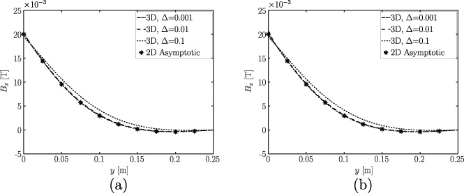(79), for which A _n is calculated from (76) and (77) as $\begin{eqnarray}\displaystyle A_{n}={\displaystyle \frac{2(1-(-1)^{n})}{n{\pi}\sinh {\mu}_{n}}},\quad n=1,2,\ldots & & \displaystyle \nonumber\end{eqnarray}$ From this figure, it is evident that the numerical solution does not change once Δ becomes as small as 10⁻² and that it agrees with the asymptotic solution. Moreover, a comparison of the (a) and (b) plots indicates that the choice of 𝛽 does not affect the solution, as was suggested by the asymptotic analysis. In addition, Fig. 8 shows the corresponding plots at z = 0.0875 m and indicates that the same trends are repeated. We can also note that Figs 7 and 8 look almost identical, principally because the boundary condition for B _x at y = 0 is independent of z.

Fig. 7.

The x-component of magnetic flux density vector, B _x, vs. distance from the stirrer, y, for z = 0 m, t = 0.06 s, x = −0.6 m, for Δ = 0.001, 0.01, 0.1, as obtained from full 3D computations and the asymptotic solution for: (a) 𝛼 = B ₀, 𝛽 = 0; (b) 𝛼 = B ₀, 𝛽 = B ₀.

Fig. 8.

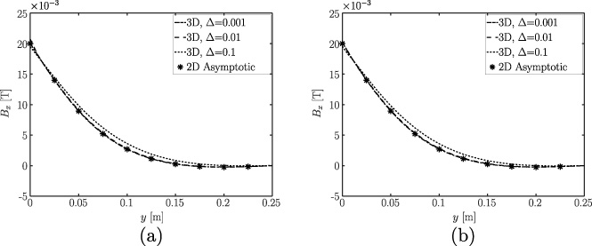
The x-component of magnetic flux density vector, B _x, vs. distance from the stirrer, y, for z = 0.0875 m, t = 0.06 s, x = −0.6 m, for Δ = 0.001, 0.01, 0.1, as obtained from full 3D computations and the asymptotic solution for: (a) 𝛼 = B ₀, 𝛽 = 0; (b) 𝛼 = B ₀, 𝛽 = B ₀.

Fig. 9.

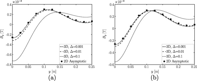
The y-component of magnetic flux density vector, B _y, vs. distance from the stirrer, y, for z = 0.0875 m, t = 0.06 s, x = −0.6 m, for Δ = 0.001, 0.01, 0.1, as obtained from full 3D computations and the asymptotic solution for: (a) 𝛼 = 0, 𝛽 = B ₀; (b) 𝛼 = B ₀, 𝛽 = B ₀.

Fig. 10.

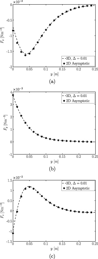
Comparison of the time-averaged component of the Lorentz force in the (a) x-direction, $\bar{F}_{x}$ , (b) y-direction, $\bar{F}_{y}$ and (c) z-direction, $\bar{F}_{z}$ vs. distance from the stirrer, y, for z = 0.0875 m, x = −0.6 m, using the asymptotic solution and the full 3D numerical solution for Δ = 0.01.

Next, Fig. 9 shows corresponding plots for B _y, this time when (𝛼, 𝛽) = (B ₀, B ₀) and (0, B ₀); here, the asymptotic solution is the numerical 2D solution for B _y and B _z. Analogous to Fig. 7, the plots indicate that the choice of 𝛽 does not affect B _y. Note that we could equally have presented plots for B _z, but plots for B _y are more instructive, since B _y was not prescribed at y = 0; hence, plots for B _y provide stronger evidence that the asymptotic limit has been reached. Observe also that this plot is for z = 0. 0875 m, rather than z = 0 m; this is because, as explained in Appendix C, B _y is odd about z = 0 as Δ →0, meaning it will be zero there. Hence, to provide a comparison at a location at which B _y is not zero, we chose the mid-plane between the axis of symmetry and the steel-air interface.

The quantities of principal interest are the time-averaged Lorentz force components, and it is therefore of interest to see whether the asymptotic approach is able to reproduce the 3D numerical approach, especially in view of the considerably smaller computational load in being able to do so. Thus, Figs 10(a)–(c) show $\bar{F}_{x},\bar{F}_{y}$ and $\bar{F}_{z}$ , respectively, for 𝛼 = B ₀, 𝛽 = B ₀, as functions of y at z = 0 m, x = −0.6 m, and given by the 3D numerical solution for Δ = 10⁻² and the leading-order asymptotic solution, i.e. $\bar{F}_{X}^{(0)},\bar{F}_{Y}^{(0)}$ and $\bar{F}_{Z}^{(0)}$ in Eq. (98). As is evident, the asymptotic solution successfully reproduces the numerical one for all three profiles. Note also that we made this comparison for Δ = 10⁻², rather than Δ = 10⁻³ as might have been expected from looking at Fig. 9, in order to demonstrate the extended range of validity of the asymptotic solution. In fact, this agreement reinforces the common experience that asymptotic solutions are often useful numerically far beyond their nominal range of validity, as discussed by Crighton [24] and Andrianov and Awrejcewicz [25].

Lastly, we point out that, although we have not presented a comparison of these results with those of [7] here, such a comparison is discussed in Appendix C.

7. Conclusions

This paper has provided an extended analysis of a recent 3D model [22] that revisited earlier theoretical work for longitudinal electromagnetic stirring in the continuous casting for steel blooms [7], in order to explore how bloom width interacts with the pole pitch of the stirrer. The work in [22] indicated the presence of a boundary layer in the steel near the interface with the stirrer, with all three components of the magnetic flux density vector being coupled to each other. In the current work, it was found that the component along the direction of the travelling wave decouples from those in the other two directions, and can even be determined analytically in the form of a series solution, regardless of the form of the boundary condition at the stirrer; this decoupling is possible because the electrical conductivity of the steel is much greater than that of the surrounding air. On the other hand, the components in the remaining two directions remain coupled and need to be calculated numerically, albeit only with a 2D simulation. Moreover, the validity of the asymptotic structure of the solution obtained was confirmed via numerical computations carried out using the finite-element software Comsol Multiphysics. Overall, the significance of this result is that the numerical work associated with the asymptotic approach is around two order of magnitude smaller than that required when performing a numerical simulation of the originally posed 3D problem.

Lastly, it is worth considering how these results would be used to simulate a real caster with longitudinal stirring. In practice, such stirring, referred to as S-EMS (strand electromagnetic stirring), is applied several metres below the mould region where solidification of the steel shell begins. Thus, in the S-EMS zone, one can expect the presence of solid, mushy and molten regions, and the magnetic field will operate across all three. From the point of view of modelling, the governing partial differential equations consist of the Maxwell’s equations, the energy equation with conduction and convection, and the turbulent Navier–Stokes equations with Lorentz force and Darcy-like damping terms, the latter to take account of the transition to the porous mushy zone and then to the solid phase that translates with uniform speed in the casting direction; see, for example, [26]. However, it is normally found that the magnetic Reynolds number, Re _m, which is given by Re _m = Vlσ𝜂, where V is a characteristic velocity scale for the flow, is small enough for the velocity to be neglected from the Maxwell equations; thus, they decouple from the Navier–Stokes equations, meaning that the components of the Lorentz force can be determined a priori. Hence, the quantities determined in this paper can be used directly in subsequent computations of the Navier–Stokes equations and energy equation.

Footnotes

α ¯ ≠ 0,β ¯ = 0

For this case, we set (A.1) $\begin{eqnarray} \displaystyle \text{} & \text{} & \displaystyle \left. \begin{array}{@{} l@{}}B_{X}=B_{X}^{(0)}+{\Delta}B_{X}^{(1)}+O({\Delta}^{2})\\ [6.0pt] {\mathcal{B}}_{X}={\mathcal{B}}_{X}^{(0)}+{\Delta}{\mathcal{B}}_{X}^{(1)}+O({\Delta}^{2}) \end{array} \right\}, \end{eqnarray}$ (A.2) $\begin{eqnarray}\displaystyle \text{} & \text{} & \displaystyle \left.\begin{array}{@{}l@{}}B_{k}={\Delta}B_{k}^{(1)}+{\Delta}^{2}B_{k}^{(2)}+O({\Delta}^{3})\\[6.0pt] {\mathcal{B}}_{k}={\Delta}{\mathcal{B}}_{k}^{(1)}+{\Delta}^{2}{\mathcal{B}}_{k}^{(2)}+O({\Delta}^{3})\end{array}\right\},\quad k=Y,Z.\end{eqnarray}$ We have, at leading order, (A.3) $\begin{eqnarray}\displaystyle \text{} & \text{} & \displaystyle -\text{i}{\mathcal{B}}_{X}^{(0)}+{\displaystyle \frac{\partial {\mathcal{B}}_{Y}^{(1)}}{\partial Y}}+{\displaystyle \frac{\partial {\mathcal{B}}_{Z}^{(1)}}{\partial Z}}=0,\end{eqnarray}$ (A.4) $\begin{eqnarray}\displaystyle \text{} & \text{} & \displaystyle 2{\pi}{\Omega}_{i}\text{i}{\mathcal{B}}_{X}^{(0)}={\displaystyle \frac{\partial ^{2}{\mathcal{B}}_{X}^{(0)}}{\partial Y^{2}}}+{\displaystyle \frac{\partial ^{2}{\mathcal{B}}_{X}^{(0)}}{\partial Z^{2}}},\end{eqnarray}$ (A.5) $\begin{eqnarray}\displaystyle \text{} & \text{} & \displaystyle 2{\pi}{\Omega}_{i}\text{i}{\mathcal{B}}_{Y}^{(1)}={\displaystyle \frac{\partial ^{2}{\mathcal{B}}_{Y}^{(1)}}{\partial Y^{2}}}+{\displaystyle \frac{\partial ^{2}{\mathcal{B}}_{Y}^{(1)}}{\partial Z^{2}}},\end{eqnarray}$ (A.6) $\begin{eqnarray}\displaystyle \text{} & \text{} & \displaystyle 2{\pi}{\Omega}_{i}\text{i}{\mathcal{B}}_{Z}^{(1)}={\displaystyle \frac{\partial ^{2}{\mathcal{B}}_{Z}^{(1)}}{\partial Y^{2}}}+{\displaystyle \frac{\partial ^{2}{\mathcal{B}}_{Z}^{(1)}}{\partial Z^{2}}},\end{eqnarray}$ subject to: at Y = 0, (A.7) $\begin{eqnarray}\displaystyle \text{} & \text{} & \displaystyle {\mathcal{B}}_{X}^{(0)}=\left\{\begin{array}{@{}ll@{}}\bar{{\alpha}}(Z) & \quad \text{for }|Z|\leq H/2\\ 0 & \quad \text{for }|Z|>H/2,\end{array}\right.\end{eqnarray}$ (A.8) $\begin{eqnarray}\displaystyle \text{} & \text{} & \displaystyle {\mathcal{B}}_{Z}^{(1)}=0;\end{eqnarray}$ at Y = 1, |Z| ≤ H∕2, (A.9) $\begin{eqnarray}\displaystyle \text{} & \text{} & \displaystyle \left[{\displaystyle \frac{{\mathcal{B}}_{X}^{(0)}}{{\eta}}}\right]_{-}^{+}=0,\end{eqnarray}$ (A.10) $\begin{eqnarray}\displaystyle \text{} & \text{} & \displaystyle [{\mathcal{B}}_{Y}^{(1)}]_{-}^{+}=0,\end{eqnarray}$ (A.11) $\begin{eqnarray}\displaystyle \text{} & \text{} & \displaystyle \left[{\displaystyle \frac{{\mathcal{B}}_{Z}^{(1)}}{{\eta}}}\right]_{-}^{+}=0,\end{eqnarray}$ (A.12) $\begin{eqnarray}\displaystyle \text{} & \text{} & \displaystyle \left[{\displaystyle \frac{1}{{\sigma}{\eta}}}\left({\displaystyle \frac{\partial {\mathcal{B}}_{Z}^{(1)}}{\partial Y}}-{\displaystyle \frac{\partial {\mathcal{B}}_{Y}^{(1)}}{\partial Z}}\right)\right]_{-}^{+}=0,\end{eqnarray}$ (A.13) $\begin{eqnarray}\displaystyle \text{} & \text{} & \displaystyle \left[{\displaystyle \frac{1}{{\sigma}{\eta}}}\left({\displaystyle \frac{\partial {\mathcal{B}}_{X}^{(0)}}{\partial Z}}\right)\right]_{-}^{+}=0;\end{eqnarray}$ at |Z| = H∕2, 0 ≤ Y ≤ 1, (A.14) $\begin{eqnarray}\displaystyle \text{} & \text{} & \displaystyle \left[{\displaystyle \frac{{\mathcal{B}}_{X}^{(0)}}{{\eta}}}\right]_{-}^{+}=0,\end{eqnarray}$ (A.15) $\begin{eqnarray}\displaystyle \text{} & \text{} & \displaystyle \left[{\displaystyle \frac{{\mathcal{B}}_{Y}^{(1)}}{{\eta}}}\right]_{-}^{+}=0,\end{eqnarray}$ (A.16) $\begin{eqnarray}\displaystyle \text{} & \text{} & \displaystyle \left[{\mathcal{B}}_{Z}^{(1)}\right]_{-}^{+}=0,\end{eqnarray}$ (A.17) $\begin{eqnarray}\displaystyle \text{} & \text{} & \displaystyle \left[{\displaystyle \frac{1}{{\sigma}{\eta}}}\left({\displaystyle \frac{\partial {\mathcal{B}}_{Z}^{(1)}}{\partial Y}}-{\displaystyle \frac{\partial {\mathcal{B}}_{Y}^{(1)}}{\partial Z}}\right)\right]_{-}^{+}=0,\end{eqnarray}$ (A.18) $\begin{eqnarray}\displaystyle \text{} & \text{} & \displaystyle \left[{\displaystyle \frac{1}{{\sigma}{\eta}}}{\displaystyle \frac{\partial {\mathcal{B}}_{X}^{(0)}}{\partial Y}}\right]_{-}^{+}=0;\end{eqnarray}$ as R → ∞, (A.19) $\begin{eqnarray}\displaystyle {\mathcal{B}}_{X}^{(0)},{\mathcal{B}}_{Y}^{(1)},{\mathcal{B}}_{Z}^{(1)}\rightarrow 0. & & \displaystyle\end{eqnarray}$

This system of equations decouples, so that ${\mathcal{B}}_{X}^{(0)}$ can be found first, and then ${\mathcal{B}}_{Y}^{(1)}$ and ${\mathcal{B}}_{Z}^{(1)}$ . In fact, the equations for ${\mathcal{B}}_{X}^{(0)}$ are identical to those given in Section 4.1, although the ones for ${\mathcal{B}}_{Y}^{(1)}$ and ${\mathcal{B}}_{Z}^{(1)}$ are different to those for ${\mathcal{B}}_{Y}^{(1)}$ and ${\mathcal{B}}_{Z}^{(1)}$ in the same section, on account of the source term in Eq. (A.3), which was not present in Eq. (51).

α ¯ = 0,β ¯ ≠ 0

For this case, we set (B.1) $\begin{eqnarray} \displaystyle \text{} & \text{} & \displaystyle \left. \begin{array}{@{} l@{}}B_{X}={\Delta}B_{X}^{(0)}+{\Delta}^{2}B_{X}^{(1)}+O({\Delta}^{3})\\ [6.0pt] {\mathcal{B}}_{X}={\Delta}{\mathcal{B}}_{X}^{(0)}+{\Delta}^{2}{\mathcal{B}}_{X}^{(1)}+O({\Delta}^{3}) \end{array} \right\}, \end{eqnarray}$ (B.2) $\begin{eqnarray}\displaystyle \text{} & \text{} & \displaystyle \left.\begin{array}{@{}l@{}}B_{k}=B_{k}^{(1)}+{\Delta}B_{k}^{(2)}+O({\Delta}^{2})\\[6.0pt] {\mathcal{B}}_{k}={\mathcal{B}}_{k}^{(1)}+{\Delta}{\mathcal{B}}_{k}^{(2)}+O({\Delta}^{2})\end{array}\right\},\quad k=Y,Z.\end{eqnarray}$ We have, at leading order, (B.3) $\begin{eqnarray}\displaystyle \text{} & \text{} & \displaystyle {\displaystyle \frac{\partial {\mathcal{B}}_{Y}^{(0)}}{\partial Y}}+{\displaystyle \frac{\partial {\mathcal{B}}_{Z}^{(0)}}{\partial Z}}=0,\end{eqnarray}$ (B.4) $\begin{eqnarray}\displaystyle \text{} & \text{} & \displaystyle 2{\pi}{\Omega}_{i}\text{i}{\mathcal{B}}_{X}^{(1)}={\displaystyle \frac{\partial ^{2}{\mathcal{B}}_{X}^{(1)}}{\partial Y^{2}}}+{\displaystyle \frac{\partial ^{2}{\mathcal{B}}_{X}^{(1)}}{\partial Z^{2}}},\end{eqnarray}$ (B.5) $\begin{eqnarray}\displaystyle \text{} & \text{} & \displaystyle 2{\pi}{\Omega}_{i}\text{i}{\mathcal{B}}_{Y}^{(0)}={\displaystyle \frac{\partial ^{2}{\mathcal{B}}_{Y}^{(0)}}{\partial Y^{2}}}+{\displaystyle \frac{\partial ^{2}{\mathcal{B}}_{Y}^{(0)}}{\partial Z^{2}}},\end{eqnarray}$ (B.6) $\begin{eqnarray}\displaystyle \text{} & \text{} & \displaystyle 2{\pi}{\Omega}_{i}\text{i}{\mathcal{B}}_{Z}^{(0)}={\displaystyle \frac{\partial ^{2}{\mathcal{B}}_{Z}^{(0)}}{\partial Y^{2}}}+{\displaystyle \frac{\partial ^{2}{\mathcal{B}}_{Z}^{(0)}}{\partial Z^{2}}},\end{eqnarray}$ subject to: at Y = 0, (B.7) $\begin{eqnarray}\displaystyle \text{} & \text{} & \displaystyle {\mathcal{B}}_{X}^{(0)}=0,\end{eqnarray}$ (B.8) $\begin{eqnarray}\displaystyle \text{} & \text{} & \displaystyle {\mathcal{B}}_{Z}^{(0)}=\left\{\begin{array}{@{}ll@{}}\bar{{\beta}}(Z) & \quad \text{for }|Z|\leq H/2\\ 0 & \quad \text{for }|Z|>H/2;\end{array}\right.\end{eqnarray}$ at Y = 1, |Z| ≤ H∕2, (B.9) $\begin{eqnarray}\displaystyle \text{} & \text{} & \displaystyle \left[{\displaystyle \frac{{\mathcal{B}}_{X}^{(1)}}{{\eta}}}\right]_{-}^{+}=0,\end{eqnarray}$ (B.10) $\begin{eqnarray}\displaystyle \text{} & \text{} & \displaystyle \left[{\mathcal{B}}_{Y}^{(0)}\right]_{-}^{+}=0,\end{eqnarray}$ (B.11) $\begin{eqnarray}\displaystyle \text{} & \text{} & \displaystyle \left[{\displaystyle \frac{{\mathcal{B}}_{Z}^{(0)}}{{\eta}}}\right]_{-}^{+}=0,\end{eqnarray}$ (B.12) $\begin{eqnarray}\displaystyle \text{} & \text{} & \displaystyle \left[{\displaystyle \frac{1}{{\sigma}{\eta}}}\left({\displaystyle \frac{\partial {\mathcal{B}}_{Z}^{(0)}}{\partial Y}}-{\displaystyle \frac{\partial {\mathcal{B}}_{Y}^{(0)}}{\partial Z}}\right)\right]_{-}^{+}=0,\end{eqnarray}$ (B.13) $\begin{eqnarray}\displaystyle \text{} & \text{} & \displaystyle \left[{\displaystyle \frac{1}{{\sigma}{\eta}}}\left(-\text{i}{\mathcal{B}}_{Z}^{(0)}+{\displaystyle \frac{\partial {\mathcal{B}}_{X}^{(1)}}{\partial Z}}\right)\right]_{-}^{+}=0;\end{eqnarray}$ at |Z| = H∕2, 0 ≤ Y ≤ 1, (B.14) $\begin{eqnarray}\displaystyle \text{} & \text{} & \displaystyle \left[{\displaystyle \frac{{\mathcal{B}}_{X}^{(0)}}{{\eta}}}\right]_{-}^{+}=0,\end{eqnarray}$ (B.15) $\begin{eqnarray}\displaystyle \text{} & \text{} & \displaystyle \left[{\displaystyle \frac{{\mathcal{B}}_{Y}^{(1)}}{{\eta}}}\right]_{-}^{+}=0,\end{eqnarray}$ (B.16) $\begin{eqnarray}\displaystyle \text{} & \text{} & \displaystyle \left[{\mathcal{B}}_{Z}^{(1)}\right]_{-}^{+}=0,\end{eqnarray}$ (B.17) $\begin{eqnarray}\displaystyle \text{} & \text{} & \displaystyle \left[{\displaystyle \frac{1}{{\sigma}{\eta}}}\left({\displaystyle \frac{\partial {\mathcal{B}}_{Z}^{(0)}}{\partial Y}}-{\displaystyle \frac{\partial {\mathcal{B}}_{Y}^{(0)}}{\partial Z}}\right)\right]_{-}^{+}=0,\end{eqnarray}$ (B.18) $\begin{eqnarray}\displaystyle \text{} & \text{} & \displaystyle \left[{\displaystyle \frac{1}{{\sigma}{\eta}}}\left(-\text{i}{\mathcal{B}}_{Y}^{(0)}+{\displaystyle \frac{\partial {\mathcal{B}}_{X}^{(1)}}{\partial Y}}\right)\right]_{-}^{+}=0;\end{eqnarray}$ as R → ∞, (B.19) $\begin{eqnarray}\displaystyle {\mathcal{B}}_{X}^{(0)},{\mathcal{B}}_{Y}^{(1)},{\mathcal{B}}_{Z}^{(1)}\rightarrow 0. & & \displaystyle\end{eqnarray}$

This system of equations decouples, so that ${\mathcal{B}}_{Y}^{(0)}$ and ${\mathcal{B}}_{Z}^{(0)}$ can be found first, and then ${\mathcal{B}}_{X}^{(1)}$ . In fact, the equations for ${\mathcal{B}}_{Y}^{(0)}$ and ${\mathcal{B}}_{Z}^{(0)}$ are identical to those given in Section 4.1, although the ones for ${\mathcal{B}}_{X}^{(1)}$ are different to those for ${\mathcal{B}}_{X}^{(0)}$ in the same section, on account of the source term in Eqs (B.13) and (B.18), which was not present in Eqs (61) and (66).

It is also of note that the new source terms that have appeared in the leading-order problems where either $\bar{{\alpha}}$ or $\bar{{\beta}}$ are identically zero in appendices B and A, respectively, turn up in different places: in Appendix A, it is in the magnetic constraint equation, whereas in this appendix it is at the steel-air interface.

Solution from Dubke et al. [ 7 ]

Nick and Vynnycky [22] showed that by replacing (13) with (C.1) $\begin{eqnarray}\displaystyle B_{x}=-B_{0}\sin ({\omega}t-{\lambda}x), & & \displaystyle\end{eqnarray}$ it is possible to obtain a solution for which B _y behaves at y = 0 in the same way as the solution of Dubke et al. [7], which is given by (C.2) $\begin{eqnarray}\displaystyle \text{} & \text{} & \displaystyle B_{x}=-{\displaystyle \frac{B_{0}}{{\lambda}}}e^{-\mathfrak{Re}({\gamma})y}\left\{\mathfrak{Re}({\gamma})\sin {\phi}+\mathfrak{Im}({\gamma})\cos {\phi}\right\},\end{eqnarray}$ (C.3) $\begin{eqnarray}\displaystyle \text{} & \text{} & \displaystyle B_{y}=B_{0}e^{-\mathfrak{Re}({\gamma})y}\cos {\phi},\end{eqnarray}$ (C.4) $\begin{eqnarray}\displaystyle \text{} & \text{} & \displaystyle J_{z}=-{\displaystyle \frac{{\sigma}_{s}{\omega}B_{0}}{{\lambda}}}e^{-\mathfrak{Re}({\gamma})y}\cos {\phi},\end{eqnarray}$ (C.5) $\begin{eqnarray}\displaystyle \text{} & \text{} & \displaystyle F_{x}={\displaystyle \frac{{\sigma}_{s}{\omega}B_{0}^{2}}{{\lambda}}}e^{-2\mathfrak{Re}({\gamma})y}\cos ^{2}{\phi},\end{eqnarray}$ (C.6) $\begin{eqnarray}\displaystyle \text{} & \text{} & \displaystyle F_{y}={\displaystyle \frac{{\sigma}_{s}{\omega}B_{0}^{2}}{{\lambda}^{2}}}e^{-2\mathfrak{Re}({\gamma})y}\cos {\phi}\left\{\mathfrak{Re}({\gamma})\sin {\phi}+\mathfrak{Im}({\gamma})\cos {\phi}\right\},\end{eqnarray}$ where $\mathfrak{Im}$ denotes the imaginary part of a complex number, ${\phi}={\omega}t-{\lambda}x-\mathfrak{Im}({\gamma})y$ and (C.7) $\begin{eqnarray}\displaystyle {\gamma}=\sqrt{{\sigma}_{s}{\eta}_{s}{\omega}\text{i}+{\lambda}^{2}}, & & \displaystyle\end{eqnarray}$ so that (C.8) $\begin{eqnarray}\displaystyle \mathfrak{Re}({\gamma})=\sqrt{{\displaystyle \frac{{\lambda}^{2}}{2}}+{\displaystyle \frac{1}{2}}\sqrt{{\lambda}^{4}+{\sigma}_{s}^{2}{\eta}_{s}^{2}{\omega}^{2}}},\quad \mathfrak{Im}({\gamma})=\sqrt{-{\displaystyle \frac{{\lambda}^{2}}{2}}+{\displaystyle \frac{1}{2}}\sqrt{{\lambda}^{4}+{\sigma}_{s}^{2}{\eta}_{s}^{2}{\omega}^{2}}}, & & \displaystyle\end{eqnarray}$ with (C.9) $\begin{eqnarray}\displaystyle \bar{F}_{x}={\displaystyle \frac{{\sigma}_{s}{\omega}B_{0}^{2}e^{-2\mathfrak{Re}({\gamma})y}}{2{\lambda}}},\quad \bar{F}_{y}={\displaystyle \frac{{\sigma}_{s}{\omega}B_{0}^{2}\mathfrak{Im}({\gamma})e^{-2\mathfrak{Re}({\gamma})y}}{2{\lambda}^{2}}}. & & \displaystyle\end{eqnarray}$

Moreover, it was demonstrated in [22] that whilst the two expressions in (C.9) agreed with the results of 3D simulations, Eqs (C.2)–(C.6) did not. However, it was also remarked that the results in the original work [7] were presented for the situation for which Δ ≈13.1, i.e. Δ ≫ 1. It is therefore of interest to see to what extent the solution in [7] is valid for the Δ ≪1 regime that this paper has focused on.

First, we may ask whether (C.1) would once again be suitable in order that B _y behaves at y = 0 in the same way as the solution in [7], i.e. B _y = B ₀ cos(ωt −𝜆x). However, we have seen already that, for Δ ≪ 1, the choice of B _x at y = 0 will not affect B _y at all; the only way to alter B _y at y = 0 would be through the choice of B _z at y = 0, which was not considered at all in [7]. If we now consider this possibility, we see that this also would not resolve the problem. In view of the geometry, it would be reasonable to take 𝛽 to be an even function of z; however, equations (106)–(112) would then permit a solution for which $\begin{eqnarray}\displaystyle B_{y}(y,z)=-B_{y}(y,-z),\quad B_{z}(y,z)=B_{z}(y,-z), & & \displaystyle \nonumber\end{eqnarray}$ meaning that B _y is an odd function of z. Hence, B _y = 0 at z = 0, which would not be able to replicate (C.3) for any choice of 𝛽(z).

Thus, overall, for the Δ ≪ 1 regime, the solution from [7] is even further removed from the actual solution than was the case for Δ ≫ 1.

References

Kim

W.S.

and Yoon

J.K.

, Numerical prediction of electromagnetically driven flow in ASEA-SKF ladle refining by straight induction stirrer, Ironmak. Steelmak. 18 (1991), 446–453.

Chung

S.I.

Shin

Y.H.

and Yoon

J.K.

, Flow characteristics by induction and gas stirring in ASEA-SKF ladle, ISIJ Intl. 32 (1992), 1287–1296.

Tzavaras

A.A.

and Brody

H.D.

, Electromagnetic stirring and continuous-casting - achievements, problems, and goals, J. Metals 36(3) (1984), 31–37.

Q.-C.

Guo

S.-J.

Zhao

Z.-H.

Cui

J.-Z.

and Zhang

X.-J.

, Numerical simulation of electromagnetic DC casting of magnesium alloys, J. Mat. Proc. Tech. 183 (2007), 194–201.

Peel

and Menet

P.Y.

, The application of MHD side stirring technology to aluminium melting furnaces for operational efficiency improvement - a case study, J. Manuf. Sci. Prod. 15 (2015), 59–67.

Spitzer

K.H.

Dubke

and Schwerdtfeger

, Rotational electromagnetic stirring in continuous-casting of round strands, Metall. Mater. Trans. B 17 (1986), 119–131.

Dubke

Tacke

K.-H.

Spitzer

K.-H.

and Schwerdtfeger

, Flow fields in electromagnetic stirring of rectangular strands with linear inductors: Part I. Theory and experiments with cold models, Metall. Mater. Trans. B 19B (1988), 581–593.

Dubke

Tacke

K.-H.

Spitzer

K.-H.

and Schwerdtfeger

, Flow fields in electromagnetic stirring of rectangular strands with linear inductors: Part II. Computation of flow fields in billets, blooms, and slabs of steel, Metall. Mater. Trans. B 19B (1988), 595–602.

Dubke

Spitzer

K.H.

and Schwerdtfeger

, Spatial-distribution of magnetic-field of linear inductors used for electromagnetic stirring in continuous-casting of steel, Ironmak. Steelmak. 18 (1991), 347–353.

10.

Tacke

K.-H.

Grill

Miyazawa

and Schwerdtfeger

, Macrosegregation in strand cast steel - computation of concentration profiles with a diffusion-model, Arch. Eisenhüttenwes. 52(1) (1981), 15–20.

11.

Tacke

K.H.

and Schwerdtfeger

, Stirring velocities in continuously cast round billets as induced with rotating electromagnetic-fields, Stahl und Eisen 99 (1979), 7–12.

12.

Zhang

Shatrov

Priede

Eckert

and Gerbeth

, Intermittent behavior caused by surface oxidation in a liquid metal flow driven by a rotating magnetic field, Metall. Mater. Trans. B 42 (2011), 1188–1200.

13.

Liu

Qiu

and Zhang

, Numerical simulation of fluid flow in a round bloom mold with in-mold rotary electromagnetic stirring, Metall. Mater. Trans. B 43B (2012), 1657–1675.

14.

Yang

Xie

Ning

Liu

and Ji

, A framework for soft sensing of liquid pool length of continuous casting round blooms, Metall. Mater. Trans. B 45 (2014), 1545–1556.

15.

Poole

G.M.

Heyen

Nastac

and El-Kaddah

, Numerical modeling of macrosegregation in binary alloys solidifying in the presence of electromagnetic stirring, Metall. Mater. Trans. B 45 (2014), 1834–1841.

16.

Ren

B.Z.

Chen

D.F.

Wang

H.D.

Long

M.J.

and Han

Z.W.

, Numerical simulation of fluid flow and solidification in bloom continuous casting mould with electromagnetic stirring, Ironmak. Steelmak. 42 (2015), 401–408.

17.

Ren

B.Z.

Chen

D.F.

Wang

H.D.

and Long

M.J.

, Numerical analysis of coupled turbulent flow and macroscopic solidification in a round bloom continuous casting mold with electromagnetic stirring, Steel Res. Intl. 86 (2015), 1104–1115.

18.

Fang

Zhang

Wang

and Lv

, The effects of a submerged entry nozzle on flow and initial solidification in a continuous casting bloom mold with electromagnetic stirring, Metals 7(4) (2017), 146, (16 pages).

19.

Fang

Wang

Zhang

and Ye

, Effects of EMS induced flow on solidification and solute transport in bloom mold, Metals 7(3) (2017), 72, (19 pages).

20.

Zhang

Zeng

Yao

Qiao

Yin

and Lu

, Modelling the rotating magnetic field with the skin effect, Intl. J. Appl. Electromagnetics Mech. 53 (2017), 283–302.

21.

Vynnycky

, On an anomaly in the modeling of electromagnetic stirring in continuous casting, Metall. Mater. Trans. B 49B (2018), 399–410.

22.

Nick

A.S.

and Vynnycky

, On longitudinal electromagnetic stirring in the continuous casting of steel blooms, J. Engng Maths 120 (2019), 129–151.

23.

Ren

Chen

Xia

Wang

and Han

, Numerical simulation of electromagnetic field in round bloom continuous casting with final electromagnetic stirring, Metals 8(11) (2018), 903, (10 pages).

24.

Crighton

D.G.

, Asymptotics - an indispensible complement to thought, computation and experiment in Applied Mathematical modelling, in: Seventh European Conf. on Mathematics in Industry, 2–6 March Fasano

and Primicerio

M.B.

(eds), Montecatini Terme. Italy, 1993, pp. 3–19.

25.

Andrianov

I.V.

and Awrejcewicz

, Asymptotic approaches in the theory of shells: Long history and new trends, in: Shell Structures, Theory and Applications: Proceedings of the 8th SSTA Conference, 12–14 October Pietraszkiewicz

and Szymczak

(eds), Jurata, Poland, 2005, pp. 3–10.

26.

Vynnycky

, Porous-media braking of electromagnetic stirring in the continuous casting of steel, in: COBEM-2017-2009, 24th ABCM International Congress of Mechanical Engineering, Curitiba, Brazil, 3–8 December, 2017.

Analysis of a model for longitudinal electromagnetic stirring in the continuous casting of steel

Abstract

Keywords

1. Introduction

2. Model formulation

2.1. Governing equations

5.1. 3D computations

Footnotes

α ¯ ≠ 0,β ¯ = 0

α ¯ = 0,β ¯ ≠ 0

Solution from Dubke et al. [ 7 ]

References