Sage Journals: Discover world-class research

Abstract

A significant part of all structural damage to conventional ships is caused by complex free-surface events like slamming, breaking waves, and green water. During these events air can be entrapped by water. The focus of this article is on the resulting air pockets affecting the evolution of the hydrodynamic impact pressure that loads the ship’s structure.

ComFLOW is a computationally efficient method based on the Navier–Stokes equations with a Volume-of-Fluid approach for the free surface, designed to perform multiphase simulations of extreme free surface wave interaction with maritime structures. We have extended ComFLOW with a Continuum Surface Force (CSF) model for surface tension, thereby completing our method for representing gas-water interaction after free surface wave impacts. The implementation was verified with benchmark cases addressing all relevant aspects of the dynamics of entrapped air pockets. The implementation was validated by means of a dam-break experiment, a characteristic model for green water impact events.

The method – having been verified and validated – was applied to a dam-break simulation for a different setting in which the impact on a wall leads to an entrapped air pocket. Surface tension was found not to have an influence on entrapped air pocket dynamics of air pockets with a radius larger than 0.08 [m]. For wave impacts it was found that the effect of compression waves in the air pocket dominates the dynamics and leads to pressure oscillations that are of the same order of magnitude as the pressure caused by the initial impact on the base of the wall. The code is available at: https://github.com/martin-eijk/2phase.git.

Keywords

CFD compressible two-phase flow Volume-of-Fluid surface tension wave impact dam-break

1. Introduction

Hydrodynamic impact loading accounts for more than 10% of structural damage to conventional ships [33]. There are multiple classes of wave impact such as those resulting from slamming, waves breaking against the structure, and green water.

In rough seas, large amounts of water can flow over the ship’s deck; this is called green water. Green water from the side of the ship has already been recorded to cause damage midships and further aft on several maritime vessels [6,32]. A green water event is illustrated in Fig. 1. During green water events involving a complex configuration of the free surface, air and water interact in a way that can lead to entrained air and entrapment of large air pockets. By entrapping an air pocket between the water and the structure, the pocket can have a cushioning effect on the peak pressure on the one hand [5,27]. On the other hand, it can give an increase of the acting force on the structure during a wave impact [5,26] and the pressure oscillations in the air pocket can increase pressure levels on the structure being impacted [27] as well as induce resonant fluid-structure interaction [3]. Naval architects are interested in determining these pressures for design.

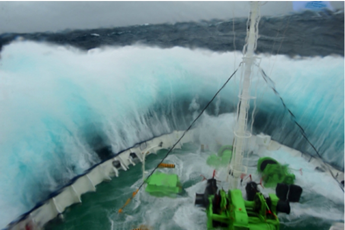
The pressures on marine structures and parts of these structures can be predicted by modelling the dynamics of both water and the entrapped compressible air. To model the interaction between water and air accurately, a sharp representation of the free surface is needed. One method capable of simulating extreme free-surface flow in a computationally efficient way is ComFLOW, which has been under development for maritime applications since [12].

Fig. 1.

Green water event after slamming (C. Sun (2013), Monsoondiaries).

ComFLOW, with its most recent implementation described by [36], is based on the Navier–Stokes equations for the motion of an aggregated fluid with varying properties to model the combination of an incompressible liquid and a compressible gas phase. A fixed Cartesian grid is used with a staggered configuration of variables within a cell. The convective term is approximated with a second-order upwind scheme and the time integration is based on a second-order Adams–Bashforth scheme. The pressure is solved from a Poisson equation, after which the velocity is solved from the newly computed pressure gradients. To describe the free surface the Volume-of-Fluid (VoF) method is used with piecewise-linear line segments to reconstruct the position of the free surface within cells (PLIC). The treatment of the density at the free surface lead to serious errors in the form of so-called spurious velocities [30], which affected the evolution of the impact pressure. A gravity-consistent averaging method for calculating the density at the cell faces was developed to prevent these spurious velocities.

We have made an implementation based on ComFLOW to investigate the effect of surface tension on the dynamics of the pressure in entrapped air pockets during wave impacts. The important aspects to entrapped air pockets are:

the position of the free surface,

surface tension,

viscosity,

compressibility.

The added value of this paper is to show the relevance of compressibility of air and surface tension during a wave impact in which an air pocket gets entrapped. The novelty of this article lies herein. With respect to [36] we have

investigated the difference between piecewise-constant (SLIC) and piecewise-linear representation (PLIC) and the role of gravity-consistent density averaging,

implemented a surface tension model based on [4],

evaluated the effect of the term $μ \nabla u^{T}$ that is often omitted in the representation of the diffusive stresses in the momentum equation

to obtain the first complete model for the representation of entrapped air pocket dynamics in wave impact events.

We have performed a verification study with a – to our knowledge – unique set of cases that test all relevant aspects of entrapped air pocket dynamics

standing capillary waves and an oscillating initially square rod that tests the combined effect of surface tension and viscosity,

a rising bubble to test for the combination of buoyancy (gravity) and surface tension,

a shock tube to test for compressibility.

The verified implementation is validated with a dam-break experiment. The implementation having been verified and validated, is used for a dam-break simulation in new setting to quantify the pressure dynamics in an entrapped air pocket. The code is available at: https://github.com/martin-eijk/2phase.git.

2. Mathematical model

The flow of two phases is modelled as an aggregated fluid with variable properties representing incompressible water and compressible air. By relaxing the pressure of the two phases to a common value, the flow can be described by one continuity equation and one momentum equation [25]. This assumption leads to a continuous velocity field. The continuity equation is given by $\begin{matrix} (1) & \int_{V} \frac{\partial ρ}{\partial t} d V + \oint_{S} (ρ u) \cdot n d S = 0, \end{matrix}$ where $u$ is the velocity vector ${[u, v]}^{T}$ , $n$ is the normal direction to the boundary of the control volume and ρ the mixture density, defined in Eq. (8).

The momentum equation in integral form is given by $\begin{matrix} (2) & \begin{matrix} \int_{V} \frac{\partial (ρ u)}{\partial t} d V + \oint_{S} ρ u (u \cdot n) d S + \oint_{S} p n d S \\ - \oint_{V} \nabla \cdot (μ (\nabla u + \nabla u^{T}) - \frac{2}{3} μ \nabla \cdot u) d V + \int_{V} ρ F d V = 0, \end{matrix} \end{matrix}$ where p is the relaxed pressure, μ is the dynamic viscosity for a mixture and F are the body forces for gravity and capillary stresses, $F = g - \frac{1}{ρ} (σ κ n δ_{Γ} - (\nabla σ) δ_{Γ})$ . The parameter κ indicates the curvature of the free-surface interface, σ is the surface tension coefficient and $δ_{Γ}$ is a delta function concentrated on the interface Γ between air and water.

The liquid is modelled as incompressible, while the density in the air is allowed to vary. This requires an additional equation with respect to solving the Navier–Stokes equations for incompressible media. Instead of solving for conservation of energy explicitly, an equation of state is used for the air density. The temperature is assumed constant, the air density is assumed barotropic, $ρ_{g} = ρ_{g} (p)$ , and the polytropic energy equation $\begin{matrix} (3) & \frac{ρ_{g}}{ρ_{0}} = {(\frac{p}{p_{0}})}^{\frac{1}{γ}}, \end{matrix}$ is used to close the system, where the polytropic coefficient $γ = 1.4$ for pure air. Instead of using $ρ_{0} = ρ^{n}$ , the initial values are used for $ρ_{0}$ and $p_{0}$ to reduce ’drift’ of the pressure [35].

The free-surface indicator function is displaced as follows: $\begin{matrix} (4) & \frac{D S}{D t} = \frac{\partial S}{\partial t} + (u \cdot \nabla) S = 0, \end{matrix}$ where $S (x, t) = 0$ gives the position of the free surface. S is not solved for directly. Instead, the volume fractions $F_{s}$ that indicate the ratio of liquid volume to cell volume are updated, after which S is reconstructed from the volume fractions.

All domain boundaries in this article are assumed closed, $u \cdot n = 0$ with n the direction normal to the domain wall, and free slip, $τ \cdot n = 0$ . The top boundary is used to define a pressure reference.

3. Numerical discretisation

3.1. Algorithm

The governing equations are discretized by means of a finite volume method on a fixed Cartesian grid with staggered variables. The velocities are defined on cell faces while the density, the pressure and the curvature are defined in cell centers.

Using cell labelling, we distinguish between the liquid phase, the gas phase and representations of structures in the domain. Cells completely filled by structures are labelled B(ody) cells. The cells filled with air are labelled E(mpty) (the E-label name is a residue from when ComFLOW was one phase). Cells with some liquid, adjacent to E-cells are labelled S(urface) cells. All other cells are labelled F(luid) cells. This means that a F-cell never connects with an E-cell. Note that a F-cell is not necessarily completely filled with liquid.

Time integration of the momentum equation is implicit for the pressure, and explicit for the convective and diffusive terms of the momentum equation. The convective and diffusive terms are integrated in time with a second-order Adams–Bashforth scheme. The time discrete version of the continuity equation is $\begin{matrix} (5) & \begin{matrix} ρ^{n + 1} + δ t ρ^{n} \nabla \cdot u^{n + 1} = ρ^{n} - δ t u^{n} \cdot \nabla ρ^{n}, \end{matrix} \end{matrix}$ and of the momentum equation $\begin{matrix} (6) & \begin{matrix} u^{n + 1} + δ t \frac{1}{ρ^{n}} \nabla p^{n + 1} \\ = u^{n} + δ t F^{n} \\ - \frac{3}{2} δ t (\frac{1}{ρ^{n}} \nabla \cdot (ρ^{n} u^{n} u^{n}) - \frac{1}{ρ^{n}} \nabla \cdot (μ^{n} (\nabla u^{n} + {(\nabla u^{n})}^{T}))) \\ + \frac{1}{2} δ t (\frac{1}{ρ^{n - 1}} \nabla \cdot (ρ^{n - 1} u^{n - 1} u^{n - 1}) \\ - \frac{1}{ρ^{n - 1}} \nabla \cdot (μ^{n - 1} (\nabla u^{n - 1} + {(\nabla u^{n - 1})}^{T}))), \end{matrix} \end{matrix}$ where n indicates the time level. The momentum equation is formulated in a non-conservative way to reduce computational cost [35].

By substituting Eq. (6) in Eq. (5), a Poisson equation for the pressure is obtained $\begin{matrix} (7) & \begin{matrix} δ t \nabla \cdot (\frac{1}{ρ^{n}} \nabla p^{n + 1}) = & \frac{1 - F_{s}^{n}}{ρ^{n}} (\frac{ρ_{g}^{n + 1} - ρ_{g}^{n}}{δ t} + \nabla \cdot {(ρ_{g} u)}^{n} - ρ_{g}^{n} \nabla \cdot u^{n}) \\ + \nabla \cdot {\tilde{u}}^{n} . \end{matrix} \end{matrix}$ The term $\tilde{u}$ is an intermediate velocity, containing contributions of the momentum terms evaluated at time level n and $n - 1$ e.g. the diffusive, convective and body force term. The first part in between parentheses on the right-hand side of Eq. (7) corresponds to the compressibility of the aggregated fluid. It represents the Lagrangian derivative of the density. Separately, these terms can be large due to the variety in density of the two phases at the free surface. Together, however, these terms need to be equal to zero for the liquid phase.

The density in the cell center at time level n is calculated by $\begin{matrix} (8) & ρ^{n} = ρ_{l} F_{s}^{n} + ρ_{g}^{n} (1 - F_{s}^{n}), \end{matrix}$ where $ρ_{l}$ and $ρ_{g}$ are the constant liquid density and the variable gas density, respectively. Because of the constant liquid density within a cell, the Lagrangian derivative of the density simplifies to $\begin{matrix} (9) & \frac{D ρ}{D t} = (1 - F_{s}) \frac{D ρ_{g}}{D t} . \end{matrix}$ When the density of the gas is much smaller than the density of the liquid, the contribution of the Lagrangian derivative to the intermediate velocity at the free surface is relatively small. The density of the gas at the next time level is found by solving Eq. (3) for $ρ_{g}^{n + 1} (p^{n + 1})$ . Before the highly non-linear term is transferred to the left-hand side of the pressure in Eq. (7), a Newton approximation is used to linearize the term $ρ_{g}^{n + 1} (p^{n + 1})$ by eliminating the power $\frac{1}{γ}$ . The pressure at the new time level is found from the linear system of equations by solving it iteratively with Gauss–Seidel.

The liquid fraction is indicated by $F_{s}$ and solved using Eq. (4) by reconstructing the free surface with SLIC in every cell. The flux through a cell face is calculated as the velocity times the area of the cell face times the time step [20].

3.2. Viscosity

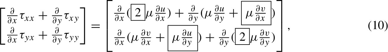
Wemmenhove [35], and also Plumerault [27], neglect the term ${(\nabla u)}^{T}$ in the viscous term, as is common to do. Wemmenhove et al. [36] do include the term in their mathematical description, but do not evaluate its effect. The effect of neglecting this term is evaluated for the 2D rising bubble case in Section 5.3. In matrix form the stresses become as follows. For readability the compressible term is left out of Eq. (6). For the final simulations in the Results section, the compressible term is included.

where τ indicates the shear stress. The boxed terms are added when the term ${(\nabla u)}^{T}$ is not neglected. As the viscosity is variable around the interface and $\nabla \cdot u \neq 0$ for air, the term $\nabla \cdot (μ (\nabla u + \nabla u^{T}))$ is not equal to $\nabla \cdot (μ \nabla u)$ as assumed by others [27,35].

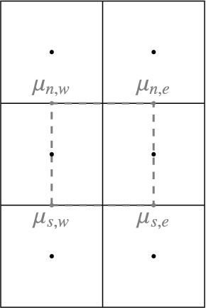
The dynamic viscosities at the top and bottom of the staggered control volume in horizontal direction are needed to find the derivative, see Fig. 2. These are found by linear interpolation between the corner point viscosity values $μ_{n, w}$ and $μ_{n, e}$ , $μ_{s, w}$ and $μ_{s, e}$ , respectively. These corner point values between adjacent cell centers are found by harmonic averaging [27]. For computing the local average viscosity at a pressure point, Eq. (8) is used for $μ (F_{s}, μ_{l}, μ_{g})$ , where $μ_{l}$ is the dynamic viscosity of the liquid and $μ_{g}$ of the gas.

Fig. 2.

Corner points of μ for staggered control volume.

4. Free-surface displacement

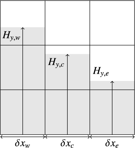
The free surface is displaced with the discretization of Eq. (4) using $F_{s}$ by calculating the fluxes at the cell faces. In [36] the free surface is reconstructed with piecewise-linear interface reconstruction (PLIC). For this article, we evaluate piecewise-constant interface representation (SLIC), with grid-aligned interfaces, and compare to PLIC, because of the significantly lower computational cost for almost the same accuracy in situations with highly distorted free surfaces such as wave impact simulations. This is in agreement with the results in Section 5.5.

4.1. Local height function

SLIC has flotsam and jetsam (small droplets disconnecting from the surface) as major drawback. As a remedy, SLIC is combined with a local height function, consisting of three cells around the S-cell in all axis directions [14]. Instead of updating the volume fraction of the S-cells separately, the height function is updated, after which the water is redistributed depending on its original surface orientation. With a local height function flotsam and jetsam are practically absent from simulations. We use the same height function to assess the local curvature for the application of surface tension.

4.2. Curvature

To implement surface tension, the curvature κ needs to be calculated in every center of a S-cell. To calculate the mean curvature, the local height function based on the surface orientation is used [20]. The grid-aligned free surface orientation is determined by rounding the gradient of the height function. When the free surface is oriented in x-direction (i.e. horizontally), the curvature for the free surface can be calculated from (see Fig. 3) $\begin{matrix} (11) & κ_{c} = \frac{1}{δ x_{c}} (\frac{\frac{\partial H_{y, e}}{\partial x}}{\sqrt{1 + {(\frac{\partial H_{y, e}}{\partial x})}^{2}}} - \frac{\frac{\partial H_{y, w}}{\partial x}}{\sqrt{1 + {(\frac{\partial H_{y, w}}{\partial x})}^{2}}}), \end{matrix}$ where $\begin{matrix} \frac{\partial H_{y, e}}{\partial x} = \frac{H_{y, e} - H_{y, c}}{\frac{1}{2} (δ x_{e} + δ x_{c})} and \frac{\partial H_{y, w}}{\partial x} = \frac{H_{y, c} - H_{y, w}}{\frac{1}{2} (δ x_{w} + δ x_{c})} . \end{matrix}$ The curvature can be determined from the height function in a similar way when the free surface is oriented in y-direction (i.e. vertically), but then with grid distances $δ y$ and the appropriate values for the height function.

Fig. 3.

Notation for curvature κ.

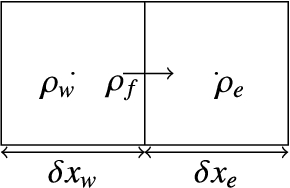
4.3. Gravity-consistent density interpolation

Like the pressure, the density is defined at cell centers. In the discretization of the governing equations, the density is also needed at the cell faces. Several alternatives for calculating the density at cell faces are available. We employ a cell-weighted average of the adjacent-cell center values, see Fig. 4 $\begin{matrix} (12) & ρ_{f} = \frac{δ x_{w} ρ_{w} + δ x_{e} ρ_{e}}{δ x_{w} + δ x_{e}}, \end{matrix}$

Fig. 4.

Notation for cell-weighted averaging.

It is demonstrated by several authors [13,16,30,36] that this method leads to spurious velocities around the free surface. From the perspective of offshore applications where the gravity force dominates, spurious velocities are caused by an imbalance between gravity and the pressure gradient.

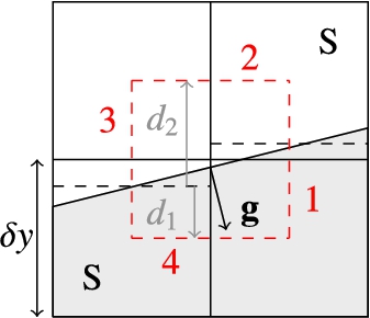
To balance these forces, both terms need to be discretized in the same way. The requirement $\nabla \times (ρ g) = 0$ can be found from the momentum equation. To solve in a way that meets the requirement, [36] came up with a gravity-consistent method (without reference to whether it is applicable for SLIC) $\begin{matrix} (13) & ρ_{f} = \frac{d_{1} ρ_{l} + d_{2} ρ_{g}}{d_{1} + d_{2}}, \end{matrix}$ where $d_{1}$ and $d_{2}$ are the distances to the free surface, see Fig. 5.

Fig. 5.

SLIC (dashed lines) of interface for density interpolation to cell faces.

Applying the gravity-consistent averaging method with SLIC, it prevents spurious velocities in many, but not all circumstances. Especially near cells with volume fractions of 0.5, the gravity-consistent method gives large errors in combination with SLIC. This because of the lower accuracy of the free surface reconstruction compared to PLIC. As an example, the requirement $\nabla \times (ρ g) = 0$ rewritten in integral form $\oint ρ g d S = 0$ is calculated, assuming that both S-cells in Fig. 5 have a volume fraction of nearly 0.5 with the same free surface orientation. This is worked out with numbers in Table 1; it gives the sum of $ρ g$ over the dashed red lines, using a gravity vector of $g = {[- 10, - 10]}^{T} [m / s^{2}]$ perpendicular to the free surface. The non-zero residue of the gravity-consistent method in Table 1 yields spurious velocities, whereas the cell-weighted method of density averaging does not. Note that besides the free surface configuration illustrated in Fig. 5, there are many other configurations that have non-zero residues, leading to spurious velocities.

Table 1

Cell-face densities multiplied by the gravity and the normal direction of the dashed line for Fig. 5

	Gravity-consistent	Cell-weighted
${(ρ g_{y})}_{1}$	−10,000	−7,500
${(ρ g_{x})}_{2}$	−10	−2,500
${(ρ g_{y})}_{3}$	10	2,500
${(ρ g_{x})}_{4}$	5,000	7,500
$\oint ρ g$	−5,000	0

The effect of the residuals in Table 1 is illustrated in Fig. 6 for a domain size of $1 [m] \times 1 [m]$ , $30 \times 30$ cells, and the orientation of the gravity vector and free surface mentioned above. The maximum spurious velocity reached after 3 [s] using the gravity-consistent method is 0.4 [m/s] while using cell-weighted density method a maximum velocity of $1 \cdot 10^{- 9} [m/s]$ is obtained. It was found that gravity-consistent density averaging combined with SLIC produces spurious velocities, just like cell-weighted averaging. The errors for cell-weighted density averaging appear to be smaller and more similar for different free surface configurations than gravity-consistent density averaging. For this reason, combined with the fact that it requires less computational effort, we chose cell-weighted averaging together with SLIC for the remainder of this article.

Fig. 6.

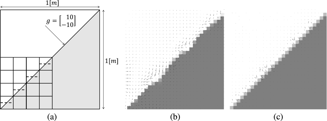
Liquid fraction- and velocity field: (b) gravity-consistent averaging (max. 0.4 [m/s]) versus (c) cell-weighted averaging (max. $1 \cdot 10^{- 9} [m/s]$ ).

4.4. Capillary forces

Because we chose an aggregated-fluid approach to keep computational costs in check, the capillary force is added to the momentum equation as a body force. Two options considered for the implementation of the body force are Continuum Surface Force (CSF) [4] and Sharp Surface Force (SSF) [13]. Of the two, SSF is formally more accurate, but CSF is less involved and has similar practical accuracy, because the error resulting from the imbalance between pressure and surface tension is dominated by how the curvature of the free surface is estimated [1].

The density in CSF is averaged between phases ( $\tilde{ρ} = \frac{1}{2} (ρ_{l} + ρ_{g})$ ) to reduce spurious velocities in high density ratio flows [4]. The delta function $δ_{Γ}$ in $F$ below Eq. (2) is equal to $| \nabla F_{s} |$ and the surface tension coefficient σ is assumed constant. The force is discretized over a (momentum) control volume consisting of two half (continuity) cells where either cell can have a surface orientation with a certain curvature. It was demonstrated by [13] that a face-centered CSF implementation performs better than a cell-centered one. Our discretization of $\int_{V} \frac{1}{ρ^{n}} F_{σ}^{n} d V$ in x-direction becomes $\begin{matrix} (14) & - \frac{1}{{\tilde{ρ}}^{n}} σ κ_{f} (F_{s, e}^{n} - F_{s, w}^{n}) δ y_{c}, \end{matrix}$ where, $\begin{matrix} κ_{f} = \{\begin{matrix} (κ_{w} + κ_{e}) / 2, & if κ_{e} and κ_{w} are defined, \\ κ_{w}, & if κ_{e} is not defined, \\ κ_{e}, & if κ_{w} is not defined . \end{matrix} \end{matrix}$ The subscripts indicate the position of the variable in the staggered control volume. An example is shown in Fig. 7, where in this case $κ_{f} = κ_{e}$ .

Fig. 7.

Cell face value of κ when using SLIC.

5. Verification and validation

Our implementation is verified with several cases chosen to test for all essential aspects of the dynamics of entrapped air pockets. They are: a 2D standing viscous capillary wave to compare the interaction of surface tension and viscosity near the free surface to an analytical solution; a 2D planar oscillating rod to compare the same interaction along the circumference of a circle with a benchmark; a 2D rising bubble to compare the interaction of buoyancy (gravity) and surface tension to a benchmark; and a 1D shock tube to compare the effect of compressibility after impacts to an analytical solution.

5.1. 2D standing viscous capillary wave

Fig. 8.

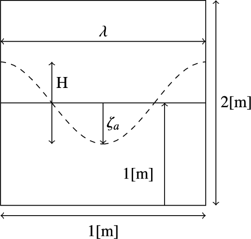
Setup for simulation of capillary wave.

Standing wave simulations can be used to asses the performance of the numerical method for free-surface waves. All important free-surface dynamics are included, while the domain is conveniently limited [34]. Standing capillary waves are driven by surface tension. We simulated them with zero gravity to verify the CSF model used for the representation of surface tension described in Section 4.4. The setup with a domain of $1 [m] \times 2 [m]$ is shown in Fig. 8. The density and the dynamic viscosity of the compressible air is $ρ_{g} = 1 {[kg/m}^{3}]$ and $μ_{l} = 0.01 [kgm/s]$ . The density and viscosity of the liquid are varied in three simulations. The dispersion relation for a non-viscous capillary wave at zero gravity is given by [22]. $\begin{matrix} (15) & ω_{0}^{2} = \frac{σ}{ρ_{l} + ρ_{g}} | k^{3} |, \end{matrix}$ where the wave number k is equal to $2 π$ over the wave length $λ = 1 [m]$ . The initial wave height H in all simulations is 0.01 [m]. The time step limit for the simulation of capillary waves is given by [4]. $\begin{matrix} (16) & δ t ⩽ \sqrt{\frac{ρ δ x^{3}}{4 π σ}} . \end{matrix}$ The analytical solution by [28] is used to compare the numerical results to, as done also by e.g. [8,9]. Note that the solution can only be used when the kinematic viscosity is the same for both fluids. Two ratios of density and dynamic viscosity of the liquid are used, indicating the ratio of top layer over bottom layer: $\bar{ρ} = ρ_{g} / ρ_{l}$ and $\bar{μ} = μ_{g} / μ_{l}$ . By varying these ratios, three sets of numerical results are compared to the analytical solutions. A CFL number of 0.01 is used to keep advection errors small [2]. The results for $σ = 1 [N/m]$ are shown in Fig. 9. The numerical results are almost identical to the analytical solution of [28], which verifies the method for the effect of surface tension. The period is almost the same as the inviscid solution in Eq. (15) if one considers that viscosity makes the wave period slightly larger.

Fig. 9.

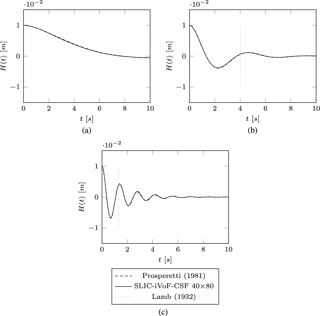
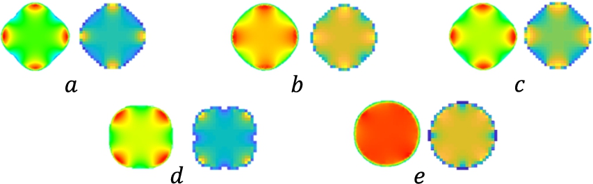
Capillary standing wave for different ratios compared with analytical solutions (a) $\bar{ρ}$ and $\bar{μ} = 1, 000$ ; (b) $\bar{ρ}$ and $\bar{μ} = 100$ ; (c) $\bar{ρ}$ and $\bar{μ} = 10$ .

5.2. 2D planar oscillating rod

Another test case for the CSF model is an initially square 2D planar rod of liquid in gas where oscillations are generated by capillary forces. This case has a direct relation to an oscillating air pocket entrapped by a wave impact. Our numerical results are compared with the results of [31] who used ANSYS Fluent.

For the simulation, a square of liquid with an area of $4 \cdot 10^{- 4} [m^{2}]$ is used. This 2D square should become, due to the capillary forces, a 2D circle with a diameter of approximately $2.26 \cdot 10^{- 2} [m]$ . The surface tension coefficient in the simulations equals $σ = 2.36 \cdot 10^{- 2} [N/m]$ . The domain size is $0.04 [m] \times 0.04 [m]$ with 40 equally spaced cells in both directions. A fixed time step of $1.0 \cdot 10^{- 3} [s]$ is used. The liquid density and gas density are unvarying and equal to $ρ_{l} = 790 [kg / m^{3}]$ and $ρ_{g} = 1.2 [kg / m^{3}]$ , respectively. The dynamic viscosity of the gas and liquid phase is $1.0 \cdot 10^{- 3} [Pa \cdot s]$ . These settings were also used by [31]. A major difference is that we used 1,600 cells, where they used 25,262 prism elements.

The simulation results are presented in terms of diameter as a function of time, shape of the rod and the pressure. The change of the rod diameter over time is compared with the results of [31] in Fig. 10(a).

Fig. 10.

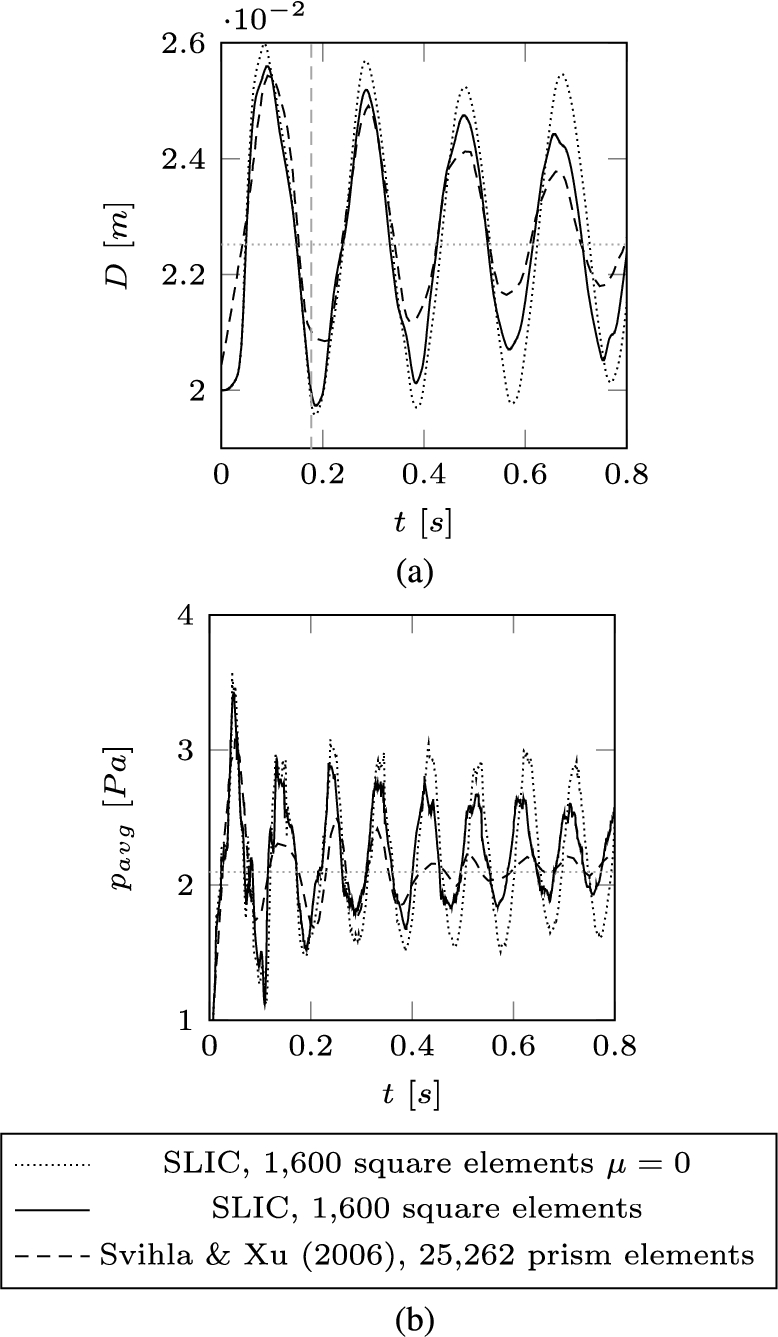
(a) Diameter and (b) average pressure of the bubble over time compared with [31].

The figure shows that the diameter oscillates towards the theoretical diameter and that the oscillations decrease over time as a result of both physical and numerical dissipation (the latter becoming less with grid refinement). The pressure in the bubble at equilibrium should be equal to $2 σ / D = 2.09 [Pa]$ . The pressure in Fig. 10(b) converges to a value somewhat higher than the analytical value due to a systematic error made for the curvature [29]. Renardy and Renardy [29] showed that the integral effect of the curvature converges to a value different than the analytical value. This is also confirmed by the results of [7] for an initially static 2D droplet. According to [15], in the inviscid limit, the angular frequency of oscillation for a 2D planar rod is given by [22] as $\begin{matrix} (17) & ω^{2} = (n) (n^{2} - 1) \frac{8 σ}{(ρ_{l} + ρ_{a}) D^{3}}, \end{matrix}$ where n is the mode of oscillation, equal to 4 for an initial square. This results in an oscillation period of $\approx 0.178 [s]$ . The period in our numerical results is smaller than 2% different from the analytical value, which we attribute mostly to the presence of viscosity in our model.

In Figs 11 and 12 the volume fraction and pressure over time are compared. Note that a different color scale is used than by [31], but these graphs are presented to demonstrate that our shape and our pressure maxima and minima match with their results, especially at the beginning. There is less of a match in Fig. 12(e). This is because the size of the oscillations in our method did not attenuate by the same amount as in [31] at the time of the snapshot; our method has less dissipation. The same conclusion is found from Fig. 10(b).

Fig. 11.

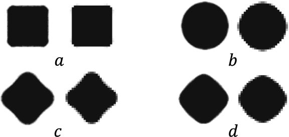
Volume fraction against time compared with [31] (left); (a) 0.01 [s], (b) 0.05 [s], (c) 0.09 [s], (d) 0.13 [s].

Fig. 12.

Pressure against time compared with [31] (left); (a) 0.49 [s], (b) 0.51 [s], (c) 0.67 [s], (d) 0.75 [s], (e) 0.79 [s].

5.3. 2D rising bubble

The following test case is for the combination of buoyancy (gravity), viscosity and surface tension. Our results are compared with the benchmark for a rising bubble [17]. This benchmark was created due the absence of analytical solutions and used for quantitative comparison of incompressible interfacial flow codes. The initial fluid configuration of the 2D rising bubble test case is shown in Fig. 13.

Fig. 13.

Flow domain for 2D rising bubble.

In the benchmark, both water and air are incompressible. The density of the water and air are 1,000 [kg/m³] and 100 [kg/m³], respectively. Further parameter values are shown in Table 2.

Table 2

2D rising bubble parameter variations. Simulation 3 corresponds to the benchmark values

Test	$μ_{w} [\frac{kg}{ms}]$	$μ_{a} [\frac{kg}{ms}]$	$σ [\frac{N}{m}]$	Re [–]
Benchmark	10	1	24.5	35
	0.01	$1 \cdot 10^{- 3}$	0	$35 \cdot 10^{3}$
	0.01	$1 \cdot 10^{- 3}$	24.5	$35 \cdot 10^{3}$
	10	1	24.5	35

The spatial mean rise velocity $v_{c}$ is found from the simulations and compared with the benchmark. It is calculated as $\begin{array}{l} (18) & v_{c} = \frac{\int_{V_{b}} v d V}{\int_{V_{b}} d V} = \frac{\sum_{b} v \cdot (1 - F_{s}) V}{\sum_{b} (1 - F_{s}) V}, \end{array}$ where $V_{b}$ is the volume of the bubble region, V the cell size, and b the number of cells which are covered by the bubble.

Before making the comparison between our implementation, the results of [36] and the benchmark, we investigated the setup with parameter variations. These simulations are indicated in Table 2 with numbers ranging from 1 to 3. For these simulations, a grid of $40 \times 120$ cells was used. Figure 14 shows the spatial mean velocity of the rising bubble for the three simulations. Figure 15 shows the different rising bubble geometries.

Fig. 14.

Spatial mean velocity for all the rising bubble cases using the original method ComFLOW with a grid size of $40 \times 120$ .

Fig. 15.

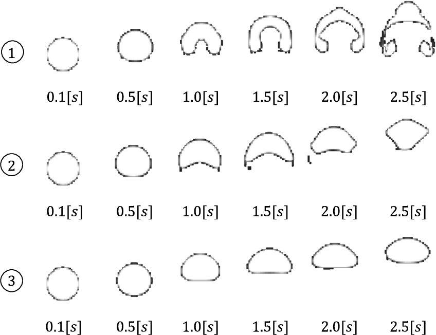
Snapshots of the 2D rising bubble in order of time for the three cases given in Table 2.

From the figures, we find that the evolution of the spatial mean velocity and the geometry of the bubble are highly dependent on surface tension and viscosity. Without surface tension (simulation 1), the rising velocity after the penetration of the jet is lower than with surface tension, because the bubble becomes wider as it rises. With a high surface tension for simulation 2, the bubble does not become as wide and does not slow down as much. The bubble reaches a higher maximum velocity and the bubble’s acceleration (after 2.2 [s]) occurs earlier in simulation 2 than in simulation 3 due to larger viscous stresses in simulation 3. Simulation 3 has the same parameters as the benchmark.

With the implementation in [35], we found by varying parameters, that we were never able to capture the benchmark’s spatial mean velocity when it is at maximum. After more careful consideration, it was concluded that the viscosity model was incomplete. Upon adding the boxed terms in Eq. (10) a better comparison with the benchmark was obtained. This is demonstrated in Fig. 16. With the same grid size of $80 \times 240$ and only the implementation of the missing viscous stress components, the difference in mean spatial velocity with the benchmark was reduced from 3.0% [35] to 0.3% (present implementation).

Fig. 16.

Spatial mean velocity compared with the benchmark of [17] with a grid resolution of $80 \times 240$ .

To investigate how our method deals with two merging interfaces, the free surface and the air-water interface of the bubble, an additional simulation was performed with a similar air bubble interface configuration and a lowered free surface. It is shown in Fig. 17 for a numerical simulation how the rising air bubble protrudes through the free surface. Note that this event was not part of the benchmark.

Fig. 17.

Snapshots of the 2D rising bubble passing through the interface in order of time.

5.4. 1D shock tube

By entrapping an air pocket between the water and the structure, the pocket is compressed and can have a cushioning effect on the peak pressure during a wave impact [5,27]. The modelling of the compressibility of the air is tested with the simulation of a shock wave. Note that in our case a non-conservative momentum equation is solved which results in diffused shock waves. The interest for our slamming applications, however, is not in the exact position of the shock, but rather on the associated pressure levels.

The simulation is based on [10], who derived an analytical solution for a 1D shock tube. The tube is simulated with unit length in two simulations. It is completely filled by gas ( $F_{s} = 0$ ), using 400 cells for one simulation and 600 cells for the other. On either side, the velocity and the gradient of the pressure are set to zero. The time step is unvarying and equal to $3.33 \cdot 10^{- 7} [s]$ and the specific ratio for air, $γ = 1.4$ . The initial values in the domain are $\begin{array}{l} p = \{\begin{matrix} 10^{6} [Pa], & x < 0.5 [m], \\ 10^{5} [Pa], & x > 0.5 [m], \end{matrix}, u = 0 [m/s], \\ ρ_{a} = \{\begin{matrix} 6.908 {[kg/m}^{3}], & x < 0.5 [m], \\ 1.33 {[kg/m}^{3}], & x > 0.5 [m] . \end{matrix} \end{array}$

Figure 18 shows the initial configuration of the shock tube, divided in a driver section with the higher pressure and a driven section with a lower pressure. The figure also shows the relevant stages of the evolution of the pressure. When released, two propagating fronts are created, moving in opposite direction, the shock front and the rarefraction. The pressure immediately upstream of the shock is called the contact surface ( $p_{2}$ ). The Mach number associated with these two pressure levels can be found from $\begin{matrix} (19) & p_{2} = p_{1} (1 + \frac{2 γ}{γ + 1} ({Ma}^{2} - 1)), \end{matrix}$ yielding a value of $Ma = 1.71$ when $p_{2} = 324 [kPa]$ .

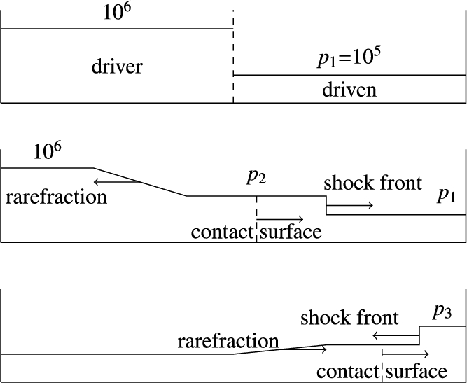
The pressure downstream of the shock after reflection from the domain wall has taken place ( $p_{3}$ in Fig. 18) can be calculated with $\begin{matrix} (20) & p_{3} = p_{2} (\frac{(α + 2) \frac{p_{2}}{p_{1}} - 1}{\frac{p_{2}}{p_{1}} + α}), \end{matrix}$ where $\begin{matrix} α = \frac{γ + 1}{γ - 1} . \end{matrix}$ This results in $p_{3} = 875 [kPa]$ .

Fig. 18.

Initial condition and relevant stages of the pressure in a shocktube simulation.

The results of the numerical simulations are plotted in Fig. 19. The figure shows the pressure in the domain for different moments in time. The simulated shock front moves with an average speed of $\approx 560 [m/s]$ which corresponds with $Ma = 1.71$ . This is in agreement with the analytical results.

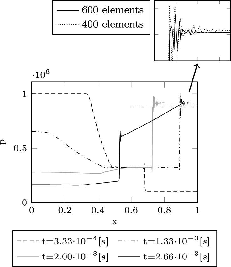
When using 400 grid cells, pressure values $p_{2} = 324 [kPa]$ and $p_{3} = 915 [kPa]$ are found. When using 600 grid cells, pressure levels $p_{2} = 324.5 [kPa]$ and $p_{3} = 908.7 [kPa]$ are found. Figure 19 shows wiggles near the shock front that originate from using central discretization of the pressure with an underresolved shock. As expected, the wiggles and the range in space over which they occur become smaller with increasing grid resolution.

Fig. 19.

(Reflected) shock front in terms of the pressure at different time levels (400 grid cells and 600 grid cells in the enlargement.

It is demonstrated that the simulation results for the 1D shock tube converge for a larger number of grid cells and that they converge to the analytical values. The wiggles observed near the shock front become smaller with an increased number of grid cells. They do not grow in time and are not expected to interfere with our interpretation of the pressure levels in wave slamming events with enclosed air pockets.

5.5. Dam-break experiment

The final comparison before moving on to our main result is for the onset of a wave impact event. The present implementation is validated against the experiments of [23] who focus on the evolution of the free surface in a dam-break event. A dam-break is a characteristic model for wave impact events.

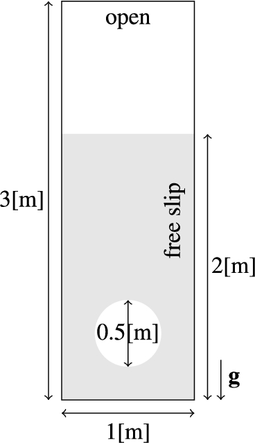
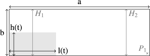
The domain and initial condition for the experiment by [23] is shown in Fig. 20. The size of the domain is $a = 0.584 [m]$ and $b = 0.350 [m]$ . The size of the dam of water is $l_{0} = 0.292 [m]$ and $h_{0} = 0.146 [m]$ . The parameters for water and air are set to $ρ_{w} = 1 \cdot 10^{3} {[kg/m}^{3}]$ , $ρ_{g} = 1 {[kg/m}^{3}]$ , $μ_{w} = 1 \cdot 10^{- 3} [kg/ms]$ and $μ_{g} = 1 \cdot 10^{- 4} [kg/ms]$ . The gravitational constant is set to $g = 9.81 {[m/s}^{2}]$ and the surface tension is equal to $σ = 7.2 \cdot 10^{- 2} [N/m]$ .

Fig. 20.

Setup dam-break 2D case.

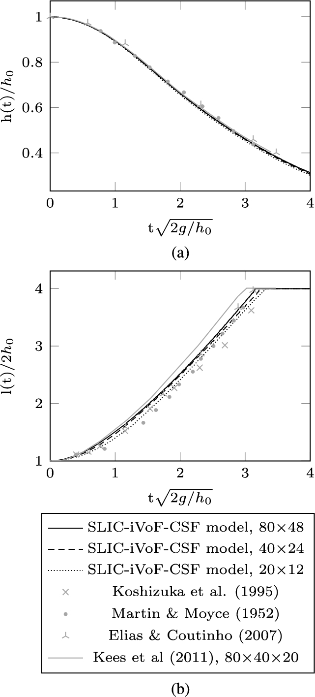
When the dam is released, the initial water level drops and a front propagates towards the opposite end of the domain. The free surface in [23] was measured along the left wall as an elevation $h (t)$ and as a position of the front $l (t)$ along the bottom. The simulation results are shown in Fig. 21, where $h (t) / h_{0}$ is plotted against dimensionless time. The simulation results are compared to the experiment of [23] as well as more recent experimental and numerical results [11,19,21]. Three different grid resolutions, $20 \times 12, 40 \times 24$ and $80 \times 48$ , were used. It is intriguing to observe that the simulation results converge away from the experimental results, i.e. the coarsest-grid simulation has the best agreement with the experiments. This is consistent with [19], but at present there is no explanation. The differences may be caused by not representing the friction between fluid and bottom well and by 3D effects [19,24].

Fig. 21.

Change of 2D dam over time in (a) height (h) and (b) length (l).

6. Main result

As mentioned, a dam-break is a representative case for wave impact phenomena, especially for green water. The objective is to demonstrate with dam-break simulations that oscillations in entrapped air pockets can cause pressure level variations of the order of the impact pressure. Our simulations are run in 2D, because of the increased likelihood of entrapping a pocket of air. Also, because the ratio of buoyancy force over viscous forces is lower in 2D, the rising velocity is smaller and air pockets persist longer. The simulation results are to be compared to the experiments conducted at MARIN (Maritime Research Institute Netherlands), in which the free surface and impact pressure on a wall in the path of the flow were measured.

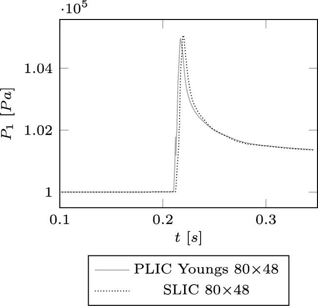
The setup of the experiment is similar to before, see Fig. 20. The domain is $a = 3.22 [m] \times b = 1.0 [m]$ and has normally a width of 1.0 [m]; the ceiling of the domain was kept open. A door was used to fill a column of water to a height of $h_{0} = 0.55 [m]$ and a width of $l_{0} = 1.22 [m]$ . The water height is measured over time with vertical wave probes at positions $H_{1} = 0.58 [m]$ and $H_{2} = 2.72 [m]$ with respect to the origin. The pressure $P_{1}$ was measured at the wall at the downstream end of the domain at a height of 0.03 [m]. Experiments were conducted as follows: the door was pulled up, releasing the water. The water flows towards the opposite domain wall. There, an impact takes place with significant run-up and overturning, after which the disturbance propagates back and forth in between the domain walls.

Fig. 22.

Difference in pressure for SLIC with height function and PLIC Youngs.

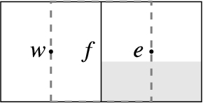
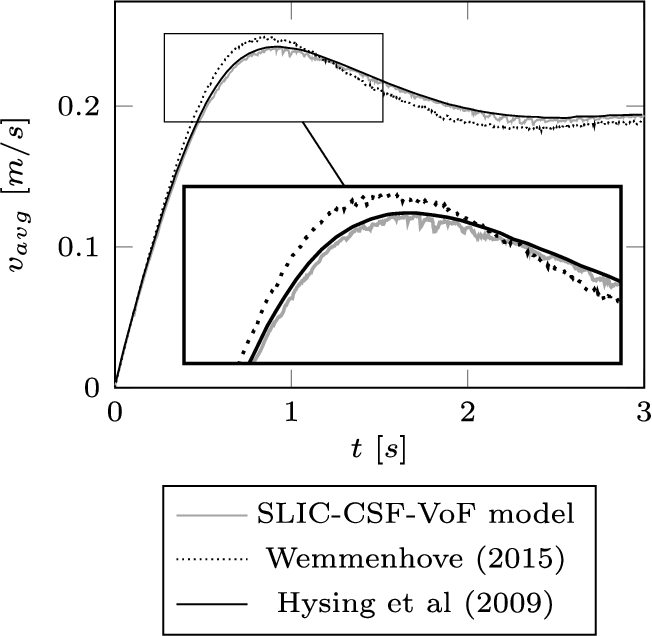
Our main interest goes out to finding the impact pressure in the most efficient way possible. A major factor determining the efficiency of the method is how the free surface is reconstructed. In the next simulation, Young’s PLIC with gravity-consistent density averaging is compared to SLIC with cell-weighted density averaging for the dam-break in the MARIN experiment. 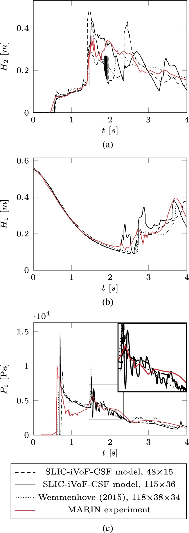The peak pressure is measured at the foot of the wall ( $P_{1}$ ). The results are shown in Fig. 22. A difference in gauge pressure ( $p - p_{0}$ ) of 2% is found, equal to 110 [Pa]. The time difference of meeting the wave is $2.3 \cdot 10^{- 3} [s]$ . This result contributes to the statement in the introduction by [35] saying that SLIC with the local height function can achieve similar results as PLIC. The results with SLIC were obtained with a factor of 3 less computational effort than PLIC, making SLIC more efficient.

Fig. 23.

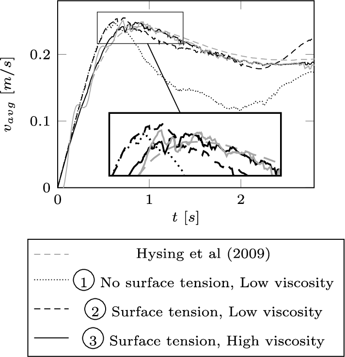
The results of the present model for the dam-break case compared with experimental results of MARIN and numerical results of [36]; (a) the water height $H_{1}$ in time, (b) the water height $H_{2}$ in time, (c) the gauge pressure $P_{1}$ .

Two more simulations were run for two different grids, $48 \times 15$ and $115 \times 36$ . The parameters for water and air at a temperature of 20° were used and the surface tension coefficient was chosen equal to $σ = 7.2 \cdot 10^{- 2} [N/m]$ . Our 2D simulation results are shown in Fig. 23, where they are compared to the 3D experiments and to the 3D results of [35]. The water heights and the pressure in Fig. 23 correspond reasonably well to the experiment and almost completely to [36], until $t = 1.54 [s]$ . It is consistent with the original method that no true convergence is observed when increasing the grid resolution.

Special attention goes out to the pressure oscillations at $P_{1}$ , see the enlargement in Fig. 23(c). These are due to the air pocket that is entrapped at around $t = 1.54 [s]$ after the run-up on the domain wall has overturned. Note that the entrapped air pocket was not part of the 3D numerical results nor the experiment. The air pocket is shown in Fig. 25 at time instance $t = 1.54 [s]$ when the pressure in the air pocket is lower than the atmospheric pressure.

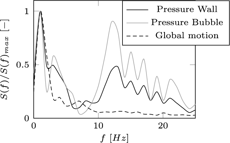
When averaging the pressure in the air pocket in space, a high frequency oscillation of 14.0 [Hz] is found. The same characteristic high frequency oscillation is found in the signal for pressure sensor $P_{1}$ at the wall. In $P_{1}$ , also a low frequency of around 3.0 [Hz] can be found. This corresponds to the global motion of the air pocket in space. By a Fourier transform of the pressure signal after 1.2 [s], the frequencies are compared. The results are illustrated in Fig. 24. The higher frequency peaks observed in Fig. 24 are due to higher harmonics and they are generated when the pocket is split in two parts [27].

Fig. 24.

Normalized Fourier transform.

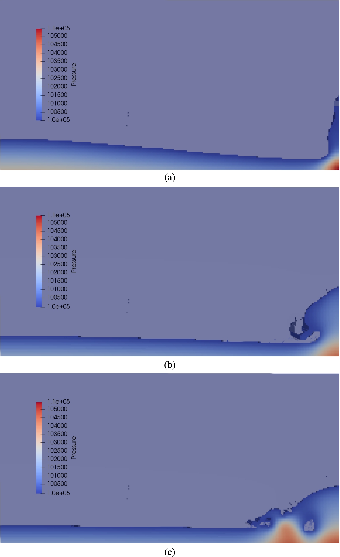
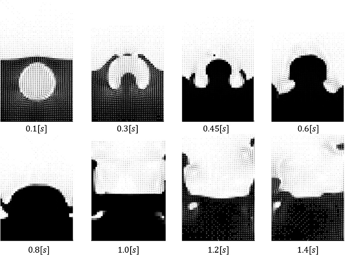
When using an equation for the natural frequency of cylindrical bubbles of this size [18] $\begin{matrix} (21) & R_{0} f_{0} = 1.10, \end{matrix}$ with $R_{0} = 0.08 [m]$ the radius of the bubble, see Fig. 25, we find a natural frequency of the bubble of $f_{0} = 14 [Hz]$ . This is of the same order of magnitude as the frequency found in the simulation. It is demonstrated that the pressure oscillations in the air pocket affect the pressure level at the wall and that the magnitude of the oscillations is of the same order as the magnitude of the impact pressure at the wall. The frequency of the oscillations is of the same order as what can be found by using simplified theory for compressible gas pockets.

Fig. 25.

Entrapment of air pocket (diameter 0.16 [m]) at 1.0 [s] (a), 1.4 [s] (b) and 1.6 [s] (c) with pressures in [Pa].

When the simulations were run without surface tension, the results were not any different. This means that compressibility and inertia govern the entrapped air pocket dynamics at this scale.

7. Conclusion

Our objective was to evaluate the effect of compressibility of air on the pressure exerted on an object during an impact with water. For this we extended the method of ComFLOW to obtain a complete model for representing the dynamics of air pockets entrapped after wave impact events. The extended implementation was verified by means of test cases relevant to the dynamics of entrapped air pockets. The extended method was validated by means of a dam-break experiment and applied to a dam-break in a new setting with a wall, in which the impact leads to an entrapped air pocket. The following conclusions were found:

PLIC does not lead to better results than SLIC for the grid resolutions used for the dam-break simulations in this article.

Gravity-consistent density averaging as in [36] does not improve the results with SLIC as it does with PLIC; cell-weighted averaging gives comparable results at lower computational cost. The combination of SLIC and cell-weighted averaging reduces the computational effort with a factor of 3 with respect to PLIC and gravity-consistent density averaging.

Our implementation compares well to test cases relevant to air pocket dynamics and compares well to dam-break experiments.

Our extended method compares well to the 3D dam-break experiment performed by MARIN until the air pocket is enclosed.

At the scale of the enclosed air pocket in our dam-break simulation (diameter 0.16 [m]), the effect of compression waves in the air dominates the dynamics.

The frequency of the pressure oscillations in the air pocket is of the same order as the analytical natural frequency of an adiabatic cylindrical bubble.

Reflecting on our main objective, we found that surface tension at this scale has no effect. Furthermore, we found that compressibility of air in an enclosed air pocket during an impact with water causes compression waves and subsequent pressure oscillations with a magnitude of the same order as the pressure of the initial impact itself.

Footnotes

Acknowledgements

The authors would like to thank Arthur Veldman of the University of Groningen for allowing us to use ComFLOW to implement our work in.

References

Abadie,

Aubin and

Legendre, On the combined effects of surface tension force calculation and interface advection on spurious currents within volume of fluid and level set frameworks, Journal of Computational Physics 297 (2015), 611–636. doi:10.1016/j.jcp.2015.04.054.

Baraldi,

M.S.

Dodd and

Ferrante, A mass-conserving volume-of-fluid method: Volume tracking and droplet surface-tension in incompressible isotropic turbulence, Computers & Fluids 96 (2014), 322–337. doi:10.1016/j.compfluid.2013.12.018.

R.W.

Bos,

J.H.

Den Besten and

M.L.

Kaminski, A reduced order model for structural response of the Mark III LNG Cargo Containment System, International Shipbuilding Progress 4 (2020), 41–56.

J.U.

Brackbill,

D.B.

Kothe and

Zemach, A continuum method for modeling surface tension, Journal of Computational Physics 100(2) (1992), 335–354. doi:10.1016/0021-9991(92)90240-Y.

Bredmose,

D.H.

Peregrine and

G.N.

Bullock, Violent breaking wave impacts. Part 2: Modelling the effect of air, Journal of Fluid Mechanics 641 (2009), 389–430. doi:10.1017/S0022112009991571.

Buchner, Green water from the side of a weathervaning FPSO, in: Proc. Conf. Offshore Mechanics and Arctic Engineering, St. John’s, 1999.

S.S.

Deshpande,

Anumolu and

M.F.

Trujillo, Evaluating the performance of the two-phase flow solver interFoam, Computational Science & Discovery 5(1) (2012), 014016.

M.S.

Dodd and

Ferrante, A fast pressure-correction method for incompressible two-fluid flows, Journal of Computational Physics 273 (2014), 416–434. doi:10.1016/j.jcp.2014.05.024.

Dong and

Wang, A rotational pressure-correction scheme for incompressible two-phase flows with open boundaries, PloS ONE 11(5) (2016), e0154565.

10.

Downes,

Knott and

Robinson, Towards a shock tube method for the dynamic calibration of pressure sensors, Phil. Trans. R. Soc. A 372(2023) (2014), 20130299.

11.

R.N.

Elias and

A.L.G.A.

Coutinho, Stabilized edge-based finite element simulation of free-surface flows, International Journal for Numerical Methods in Fluids 54(6–8) (2007), 965–993. doi:10.1002/fld.1475.

12.

Fekken,

A.E.P.

Veldman and

Buchner, Simulation of green-water loading using the Navier–Stokes equations, in: Proceedings 7th Intern. Conf. on Numerical Ship Hydrodynamics, Nantes, 1999.

13.

M.M.

Francois,

S.J.

Cummins,

E.D.

Dendy,

D.B.

Kothe,

J.M.

Sicilian and

M.W.

Williams, A balanced-force algorithm for continuous and sharp interfacial surface tension models within a volume tracking framework, Journal of Computational Physics 213(1) (2006), 141–173. doi:10.1016/j.jcp.2005.08.004.

14.

Gerrits, Dynamics of Liquid-Filled Spacecraft: Numerical Simulation of Coupled Solid–Liquid Dynamics, 2001.

15.

Ham and

Y.-N.

Young, A Cartesian adaptive level set method for two-phase flows, Technical report, Center for Turbulence Research, 2003.

16.

D.J.E.

Harvie,

M.R.

Davidson and

Rudman, An analysis of parasitic current generation in volume of fluid simulations, Applied Mathematical Modelling 30(10) (2006), 1056–1066. doi:10.1016/j.apm.2005.08.015.

17.

S.-R.

Hysing,

Turek,

Kuzmin ,

Parolini,

Burman,

Ganesan and

Tobiska, Quantitative benchmark computations of two-dimensional bubble dynamics, International Journal for Numerical Methods in Fluids 60(11) (2009), 1259–1288. doi:10.1002/fld.1934.

18.

Y.A.

Ilinskii,

E.A.

Zabolotskaya,

T.A.

Hay and

M.F.

Hamilton, Models of cylindrical bubble pulsation, The Journal of the Acoustical Society of America 132(3) (2012), 1346–1357. doi:10.1121/1.4730888.

19.

C.E.

Kees,

Akkerman,

M.W.

Farthing and

Bazilevs, A conservative level set method suitable for variable-order approximations and unstructured meshes, Journal of Computational Physics 230(12) (2011), 4536–4558. doi:10.1016/j.jcp.2011.02.030.

20.

K.M.T.

Kleefsman,

Fekken,

A.E.P.

Veldman,

Iwanowski and

Buchner, A volume-of-fluid based simulation method for wave impact problems, Journal of Computational Physics 206(1) (2005), 363–393. doi:10.1016/j.jcp.2004.12.007.

21.

Koshizuka, A particle method for incompressible viscous flow with fluid fragmentation, Comput. Fluid Dyn. J. 4 (1995), 29–46.

22.

Lamb, Hydrodynamics, Cambridge University Press, 1932.

23.

J.C.

Martin,

W.J.

Moyce,

A.T.

Price and

C.K.

Thornhill, Part IV. An experimental study of the collapse of liquid columns on a rigid horizontal plane, Phil. Trans. R. Soc. Lond. A 244(882) (1952), 312–324. doi:10.1098/rsta.1952.0006.

24.

Mohd,

M.M.

Kamra,

Sueyoshi and

Hu, Three-dimensional free surface flows modeled by lattice Boltzmann method: A comparison with experimental data, Evergreen 4 (2017), 29–35.

25.

Murrone and

Guillard, A five equation reduced model for compressible two phase flow problems, Journal of Computational Physics 202(2) (2005), 664–698. doi:10.1016/j.jcp.2004.07.019.

26.

Obhrai,

Bullock,

Wolters,

Müller,

Peregrine,

Bredmose and

Grüne, Violent wave impacts on vertical and inclined walls: Large scale model tests, in: Coastal Engineering 2004 (in 4 volumes), World Scientific, 2005, pp. 4075–4086. doi:10.1142/9789812701916_0329.

27.

L.R.

Plumerault, Numerical modelling of aerated-water wave impacts on a coastal structure, PhD thesis, University of Pau and Pays de l’Adour, 2009.

28.

Prosperetti, Motion of two superposed viscous fluids, The Physics of Fluids 24(7) (1981), 1217–1223. doi:10.1063/1.863522.

29.

Renardy and

Renardy, PROST: A parabolic reconstruction of surface tension for the volume-of-fluid method, Journal of Computational Physics 183(2) (2002), 400–421. doi:10.1006/jcph.2002.7190.

30.

Rudman, A volume-tracking method for incompressible multifluid flows with large density variations, International Journal for Numerical Methods in Fluids 28(2) (1998), 357–378. doi:10.1002/(SICI)1097-0363(19980815)28:2<357::AID-FLD750>3.0.CO;2-D.

31.

C.K.

Svihla and

Xu, Simulation of free surface flows with surface tension with ANSYS CFX, in: 2006 International ANSYS Conference, Pittsburg, 2006.

32.

T.M.

Vestbøstad, Relative wave motion along the side of an FPSO hull, in: Proceedings of the 18th Conference on Offshore Mechanics and Arctic Engineering (OMAE’99), 1999.

33.

Wang,

Tang,

Shin et al., A direct calculation approach for designing a ship-shaped FPSOs bow against wave slamming load, in: The Twelfth International Offshore and Polar Engineering Conference, 2002.

34.

P.R.

Wellens, Wave simulation in truncated domains for offshore applications, PhD thesis, Delft University of Technology, 2012.

35.

Wemmenhove, Numerical simulation of two-phase flow in offshore environments, PhD thesis, University of Groningen, 2008.

36.

Wemmenhove,

Luppes,

A.E.P.

Veldman and

Bunnik, Numerical simulation of hydrodynamic wave loading by a compressible two-phase flow method, Computers & Fluids 114 (2015), 218–231. doi:10.1016/j.compfluid.2015.03.007.

A compressible two-phase flow model for pressure oscillations in air entrapments following green water impact events on ships

Abstract

Keywords

1. Introduction

3. Numerical discretisation

3.1. Algorithm

3.2. Viscosity

4.1. Local height function

4.2. Curvature

5.1. 2D standing viscous capillary wave

Footnotes

Acknowledgements

References