Sage Journals: Discover world-class research

Abstract

Dementia, a neurodegenerative disorder, is more prominent among elderly people. This disease is one of the primary contributors amongst other diseases having a high social impact in continents of Europe and America. Treatment of the neurological disorders of dementia patients have become possible due to the Advances in medical diagnosis as in the use of Magnetic Resonance Imaging (MRI). Artificial Intelligence (AI) and Machine Learning (ML) techniques have provided solutions that enable fast, accurate and autonomous detection of diseases at their early stage. This in turn has improvised the entire health care system. This study proposes a diagnostic method, based on ML, for detecting dementia disease. The Open Access Series of Imaging Studies (OASIS) database and Alzheimer’s dataset (4 class of images) have been used for testing and training of various ML models. This involves the classification of the dependent variable into demented and non-demented patient. ML models as in Support Vector Machine (SVM), Logistic Regression, Naïve Bayes, k-nearest neighbor (KNN), Random Forest, Adaptive Boosting (ADA boost), Gradient Boosting, XG Boost, were trained and tested using OASIS dataset. Models were trained with 70% of data and tested on 30% of data. Hyper tuning of parameters of these models was also carried out to check for improvement in the results. Analysis showed that Naïve Bayes was the best amongst all giving 95% accuracy, 98% precision, 93% recall and 95% F1-score.

Keywords

Dementia OASIS Machine learning algorithms feature selection Hyper parameter tuning Naïve Bayes

1. Introduction

Dementia is a slowly advancing, fatal and complex disease, wherein the disorder in brain affects a person’s cognitive characteristics e.g., loss of thinking ability and remembering things, lack of attention, lack of logical reasoning, and other mental abilities as in difficulty in making decisions which in turn hinders the day today activities of a person [1]. Alzheimer’s disease (AD), vascular dementia, Parkinson’s disease, dementia with Lewy bodies (abnormal deposition of protein inside the nerve cells), frontotemporal dementia, and Huntington’s disease are various forms of dementia [2]. This disease is found to be more prevalent in elderly people, affecting 47.5. Millions of people. AD alone accounts for 60–80% of cases of dementia in the UK. It is estimated that currently dementia is affecting approximately 850,000 people and this count will reach 1million by 2025 and 2 million by 2051. Identifying this disease and predicting its future course is a complex task. Diagnosis involves cognitive assessment, knowing the medical history, and neuroimaging for conclusive diagnosis [3]. Clinicians use different tests to detect if a patient is showing early symptoms of dementia. The Mini-Mental State Examination (MMSE) along with set of accompanied tests proves to be more conclusive in predicting if the patient might be converting from mild cognitive impairments (MCI) to dementia [4]. Automated diagnostic systems are being designed with efficient dementia predictive models to enable detection of early dementia in patients so that prompt treatment can be provided to such patients. These ML approaches use the Electronic Health Records (EHR) already available as well as those which are being generated on a regular basis for more accurate predictions. Researchers have conducted systematic literature reviews discussing the progress of automated diagnostic systems.

2. Literature survey

Over a decade, researchers have proposed various ML algorithms for designing automated solutions for early detection of Dementia. The Naive Bayes algorithm is used for calculating the probability defined by the number of values and the frequency for a given data set [5]. It uses Bayes’ theorem. In random forests, tree predictors are combined, where each tree depends on the value of an independently sampled random vector, and all trees have the same distribution [6]. SVM, a supervised learning technique for classification. It defines an optimal hyperplane [7]. Another ensemble algorithm-ADA boost wherein the model learns from different slow learners and builds a fast learner from the mistakes of different slow learners [8]. This classifier has emerged from the decision tree. It increases the performance of models by using optimization techniques. Gradient Boosting increases the performance of weak learner/slow learner classifier boosting classifiers such as ADA boost [9]. Another algorithm KNN (K-Nearest Neighbor), a supervised ML algorithm, retrieves the closest observation from the training dataset using a Euclidean distance which is a distance metric [10].

Early detection and correct diagnosis can lead to disease-modifying therapies that slow disease progression and reduce stress and morbidity for patients and caregivers. Various ML algorithms have been widely used to supply solutions to today’s life problems of different areas [11, 12]. Optimal solutions can be achieved by hyper-parameter tunning of a machine learning algorithm. Researchers in [13] used GridSearchCV (), as a cross-validation technique. In another study, hyperparameter tuning models were used taking into consideration the factors such as age, sex, and education. There was a 96% increase in computational efficiency, which could help elucidate future diagnostic applications of Alzheimer’s disease biomarkers [14].

A study was conducted on the OASIS dataset, labeling the diagnoses into two groups: demented and non-demented [15]. 92.39% accuracy was achieved using deep learning (DL) model. In another study, an ensemble of SVMs was proposed to diagnose multivariate classification of dementia [16]. Several studies have used ML algorithms for precise detection of Parkinson’s and AD in patients. In [17], the author implemented ML algorithms on the UCI dataset to detect Parkinson’s disease. The study achieved 86% accuracy for SVM, 95% accuracy for KNN, and 90% accuracy for LDA algorithms. In [18], the author used the NACC uniform data set and four machine learning models (LR, SVM, RF, and XGB) to find Parkinson’s disease. The study achieved an accuracy of 92% for all algorithms. The authors investigated the use of a gradient boosting and artificial neural network (ANN) stacking in [19], to predict dementia in a longitudinal collection of OASIS-MRI dataset consisting of both demented and non-demented subjects. This supplied an accuracy of 89%.

As in [20], the authors utilized a 2-stage classifier, with GNB classifier used in the initial stage for classification of objects between AD, MCI, and NC, and the SVM and DT algorithms were used in later stages for analyzing the object based on the performance of the previous stage. The researchers of [21] studied the use of various ML algorithms for predicting AD. It achieved an accuracy of 83%. In [22], the authors used health behavior and medical service usage data and proposed a deep neural network (DNN) model for predicting dementia. The proposed method, DNN/scale PCA, was compared with five known ML algorithms and showed better results with 85.5% of area under the curve (AUC). Authors in [23] used a 37-item questionnaire and three feature selection methods for identification of notable features for developing diagnostic models. The authors tested six classification algorithms, and Naive Bayes outperformed all others supplying 0.81 accuracy rate, 0.82 precision rate, a 0.81 recall rate, and 0.81 F-measure. In [24], the authors used convolutional neural networks (CNNs) to detect abnormal behaviors associated with dementia. Comparing the performance of CNNs with other models as in Naive Bayes (NB), Hidden Markov Models (HMM) and Hidden Semi-Markov Models (HSMM), showed that CNNs are competitive with HMM and HSMM. In another study [25], researchers used dataset of the Survey of Health, Ageing, and Retirement in Europe (SHARE) and the PREVENT Dementia program for developing prediction models using RF and XGboost algorithms. The models achieved accuracies of 85.0% and 87%, respectively. In [26]4, the authors have proposed 7 ML models for dementia detection using MRI and demographic data from the OASIS Brains 1 dataset. The models were compared in accuracy and prediction time, and the XGB algorithm provided the highest accuracy of 97.87 and with prediction time of 0.031 seconds/sample. The studies of [27] aimed to find dementia in patients using various machine learning models. The system was evaluated with and without fine-tuning, and the SVM model is the most efficient detecting algorithm for dementia detection. The researchers of [28] proposed a modified Random Forest (m-RF) algorithm thereby classifying normal people and those at risk of AD. This algorithm achieved an accuracy of 96.43%, outperforming other algorithms. Furthermore, in [29], the proposed framework is based on a supervised learning classifier to classify subjects with dementia as AD or non-AD based on longitudinal brain MRI features. The gradient boosting algorithm outperformed giving accuracy of 97.58%. In [30], the authors proposed DL with long-short-term memory (LSTM) networks as a classifier for detecting movement patterns, including direct, rate, patch and random. The experimental results showed that deep LSTM classifiers outperformed the traditional ML classifiers, suggesting the potential use of this method in applications in healthcare areas such as in dementia detection. The authors of [31] conducted performance analysis of various ML techniques for dementia detection, with help of a clinical dataset. The study found that SVM and RF algorithms performed best on datasets from open-access repositories. Researchers of [32] used GridSearchCV () to hyper tune parameters of different ML algorithms using GSCV (). Authors in [33] discussed a high-performance multi-core SVM Hyper-parameter tuning workflow detecting AD. This resulted in a 96% increase in computational efficiency. Authors implement pre-trained language models based on transformers such as BERT and ERNIE in [34]. In [35] various computational algorithms were used for diagnosing dementia at early stage as well as at its various stages like amnestic early mild cognitive impairment (EMCI) and AD. This proved to be beneficial for checking the intensity of the disease in the patients. An accuracy of 92.5% for non-cognitive group and 75.0% for early mild cognitive impairment group, and accuracy of 93.0% for non-cognitive group and 90.5% for group with Alzheimer disease, were achieved using SVM algorithms and CNN networks.

The Sydney Memory and Ageing Study (MAS) which decides the effects of aging on cognition and Alzheimer’s Disease Neuroimaging Initiative (ADNI) which finds biomarkers for the early detection and tracking of Alzheimer’s disease [36]. Their models achieved better performance giving an accuracy of 82% for MAS and 93% for ADNI data sets, respectively. In [37], authors proposed a Decision Tree Classifier with Hyper Parameters tuning (DTC-HPT). The correctness AD classification by DTC-HP the T with accuracy of 99.10%. Here in [38], researchers discussed several symptom-based early detection methods for dementia. A synthetic minority oversampling technique (SMOTE) supplied the solution to the problem of imbalanced classes in the dataset. The proposed learning system resulted in a classification accuracy of 90.23%. In [39] authors found clusters of cognitive assessment features for optimization of the detection of mild impairment.

This study focuses on comparison of performance of ML models to find the optimized model for predicting dementia. Two methods were used in this work. One used the OASIS Longitudinal dataset and the other used the Alzheimer’s MRI dataset. Various ML models such as boosting model, logistic regression, KNN, SVM, naive bayes were trained and a comparative analysis of 8 machine learning models with and without hyper tuning of their parameters was done. Later, the Alzheimer’s MRI image dataset was used to train the SVM model.

3. Proposed methodology 1 (numeric dataset)

In method I, the following 5 procedures were carried out: Data Collection, Data Preprocessing, Data Analysis, Model Selection and Performance Evaluation using OASIS – Longitudinal Dataset. Figure 1 depicts the Proposed method for OASIS-Longitudinal Dataset.

Figure 1.

Proposed method 1.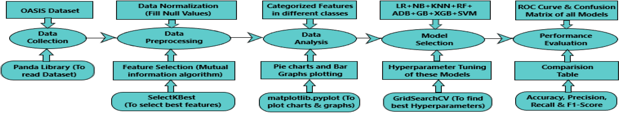

The steps involved in the first method have been discussed in the following sections.

3.1 Data collection

This work was conducted using the OASIS – Longitudinal collection of MRI datasets including right-handed (R) demented and non-demented subjects aged 60–96 years. The sample size consisted of data of 150 subjects both male and female who had attended scanning sessions once a year for 2 consecutive years. There were in all 373 MR sessions. Main Features taken into consideration from the OASIS dataset include age, gender, education, socioeconomic status, mini-mental state exam (MMSE), clinical dementia rating (CDR), Atlas scaling factor (ASF), estimated total intracranial volume (eTIV), and normalized total brain volume (nWBV). The clinical dementia rating (CDR) score is taken into consideration for classification. If the CDR score is greater than 0, the person has dementia. CDR $=$ 0, shows that the patient does not have dementia. Hence it is a binary classification problem.

Table 1
Top 5 rows of OASIS – longitudinal Dataset

Subject ID	MRI ID	Group	Visit	MR delay	M/F	Hand	Age	EDUC	SES	MMSE	CDR	eTIV	nWBV	ASF
S2_0 001	OAS2_0001_ MR1	Non-demented	1	0	M	R	87	14	2.0	27.0	0.0	1987	0.696	0.883
S2_0 001	OAS2_0001_ MR2	Non-demented	2	457	M	R	88	14	2.0	30.0	0.0	2004	0.681	0.876
S2_0 002	OAS2_0002_ MR1	Demented	1	0	M	R	75	12	NaN	23.0	0.5	1678	0.736	1.046
S2_0 002	OAS2_0002_ MR2	Demented	2	560	M	R	76	12	NaN	28.0	0.5	1738	0.713	1.010
S2_0 002	OAS2_0002_ MR3	Demented	3	1895	M	R	80	12	NaN	22.0	0.5	1698	0.701	1.034

Table 1 shows the top five rows of OASIS longitudinal. Dataset in which all 15 features are shown with their respective values.

3.2 Data pre-processing

Data preprocessing is the process for data clean-up. In this study, data is cleaned by filling in the null values and Categorical Values are replaced by numerical values. Relevant features are selected to avoid overfitting. Features are selected by the Filter methods using information gain. Figure 2 shows the most relevant features in which there is a high correlation between CDR and the target variable. The top 6 best features are selected to avoid overfitting as well as underfitting.

Figure 2.

Correlation chart of all features.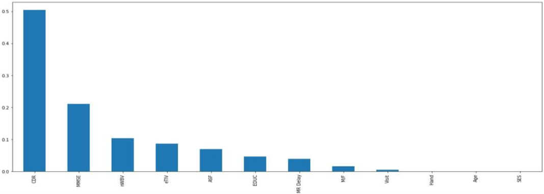

Figure 3.

(a) Histogram of CDR Parameter Figure 3: (b) Pie Chart of Group Parameter.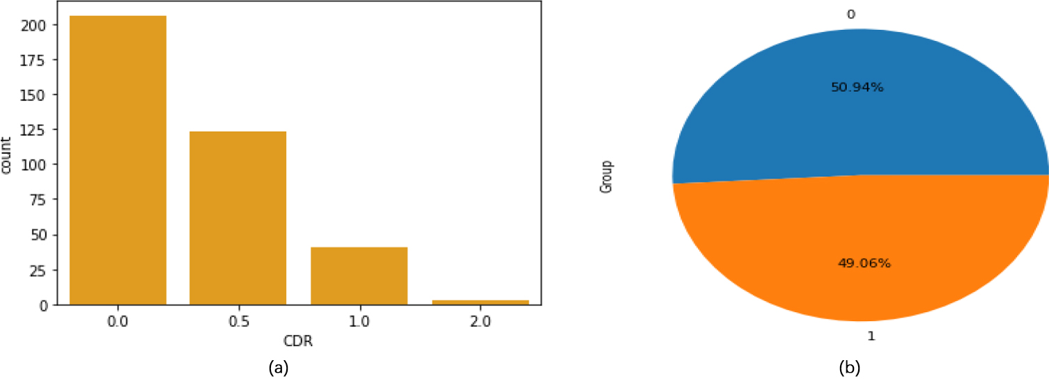

Figure 4.

Analysis of CDR parameter.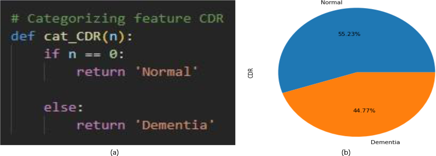

3.3 Data analysis

Figure 3(a) shows the Histogram of CDR feature. In which about 200 people have CDR value 0 that means they are normal. 0.5 value shows that about 125 people have mild dementia. 1.0 shows that about 40 people have Moderate Dementia and 2.0 value shows that about 10 people have Severe Dementia.

Figure 3(b) shows the Pie chart of Group Parameter in which blue shows the percentage of non-demented people whereas orange shows the percentage of Demented people which means 190 people are normal whereas 183 people are suffering from dementia.

In this work, CDR feature is categorized in two classes which are Normal and Demented as shown in Fig. 4. Criteria for categorizing is that if CDR value is 0 then person is normal otherwise person is suffering from Dementia.

Figure 5.

Analysis of MMSE parameter.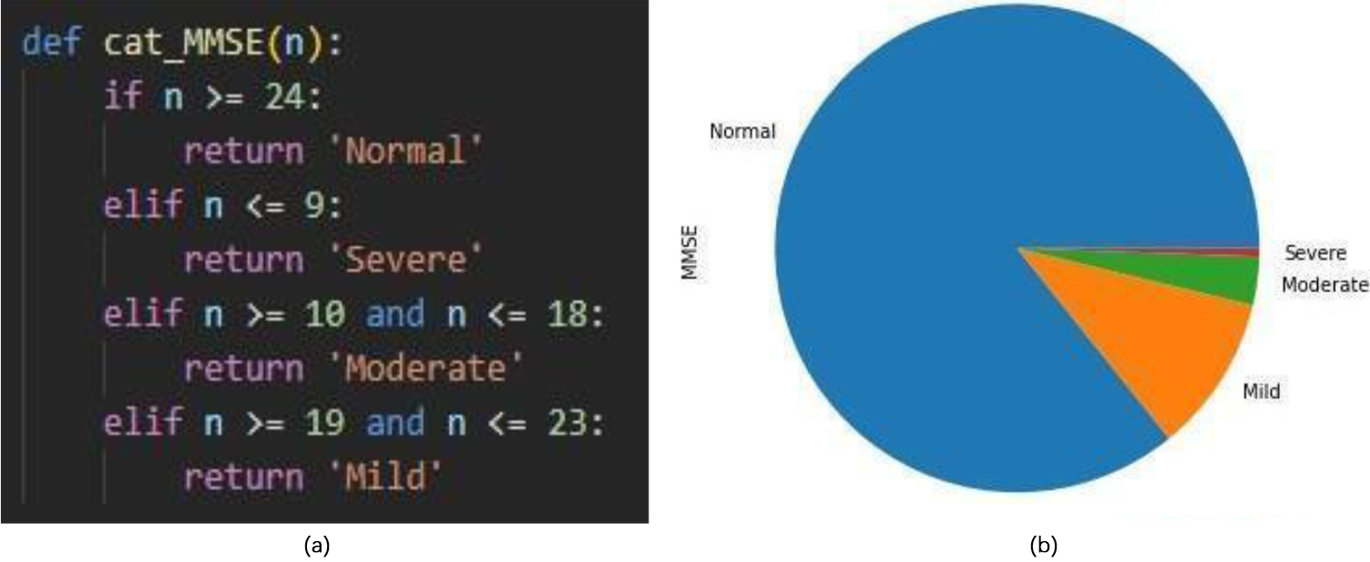

Figure 5 shows the scores of the MMSE. The highest value of MMSE obtained is 30 Count. MMSE score in range of 25 and above classifies the patient to be normal. MMSE score below 24 classifies as abnormality which shows that the patient may have cognitive impairments.

3.4 Model selection

Data analysis is followed by a crucial step, modeling for model selection. This process involves selection of one model for a prediction problem. In this article, the problem is to predict demented or non-demented people. This is a classification problem. The dependent variable is discrete in classification problems.

In this study, 15 machine learning algorithms were implemented. These models are:

•
Logistic regression

Logistic Regression (LR), involving low computational complexity is a popular ML technique used to model the probability of occurrence of a particular class. Here, the input variables need not be scaled. For each real value input, the function maps a probability value on a scale between 0 and 1 [40]. Sigmoid function is used.

$\displaystyle S\left(x\right)=\frac{1}{1+e^{-x}}$ (1)

Where, $S(x)$ stands for sigmoid function and e is Euler’s number and $x$ is independent variable.
•
Logistic regression – Hyper parameter tuning

Logistic Regression doesn’t have any key hyperparameters to be tuned. The default penalty value is ‘l2’ penalty in [‘none’, ‘l1’, ‘l2’, ‘elasticnet’]. Parameter C controls penalty intensity and the default value of parameter C is 1.0.
•
Naive Bayes

Naive Bayes (NB) classifiers are based on Bayes’ theorem. NB does not require iterative parameter estimation, thereby minimizing the computational complexity. It has a linear scaling of parameters as per the count of features. This minimizes the complexity of the model. However, the simplicity of such models relies on the assumption of non-correlation between all features, which is rarely the case [41]. For continuous-valued features a normal distribution is used i.e., Naive Bayesian Gaussian calculation method. While binary feature data can be measured using a naive Bernoulli Bayesian model [42].
•
KNN

The KNN algorithm relies on the “similar things” assumption. A Bayesian classifier will be used to predict qualitative responses [43]. For real-time data, a Bayer classifier can’t be used as it cannot know the conditional distribution of Y given X, nor can it classify a given opinion into a class with a high-level estimated probability. Euclidean distance is calculated in KNN to find the nearest neighbor. Equation to find the Euclidean distance is.

$\displaystyle\textit{Euclidean distance}=\sqrt{\left({X1-X2}\right)^{2}+\left(% {Y2-Y1}\right)^{2}}$ (2)
•
KNN – Hyper parameter tuning

The number of neighbors (n_neighbors) is the most important hyperparameter of KNN. Tests for at least one value between 1 and 25, possibly only odd numbers. The default value of n_neighbors is 5. n_neighbors in [1 to 25]. Another default value for the metric is “minkowski”. Metrics in [’euclidean’, ’manhattan’, ’minkowski’].
•
Random forest

The Random Forest algorithm, an ensemble learning method, generates different decision trees. The average of the results provided by the different decision trees is considered as final output. Individual decision trees are prone to overfitting and have high variance. Overfitting is controlled by training the decision trees on different subsamples of dataset cases [44]. Random forest models do not supply explanations for each individual test instance classification [45].
•
Random forest – Hyper parameter tuning

An important random forest parameter is n_estimators. It denotes the total number of trees in the forest. Its default value is 100. This parameter is tested on a value of 10 to check model performance. Another important parameter is the standard. It is a function that measures the quality of the distribution. This setting is tree specific. The default is “gini”.
•
ADA boost

ADA Boosting is an iterative ensemble learning system. It proves to be an efficient boosting classifier with higher accuracy as it has a sequential combination of multiple base/weak classifiers [46]. In the ADA boost algorithm defines the weights of a classifier and trains them on sample data at each iteration to accurately predict anomalous observations with minimal error [47].
•
ADA Boost – Hyper parameter tuning

The parameter settings for the test model are learning rate, n_estimators and algorithm.

The learning_rate is defined as the weight applied at each boosting iteration to each classifier. The contribution of each classifier is increased by a high learning rate. The value must be in the range (0.0, infinity).

learning rate (default $=$ 1.0)

Another important parameter is the algorithm. Default is ‘SAMME.R’. Algorithm in [‘SAMME’, ‘SAMME.R’].
•
Gradient Boosting

The Gradient Boosting (GB) model is an ensemble ML algorithm, using a gradient boosting framework and is built on top of decision trees. The authors of [48] implemented a gradient boosting machine (GBM) model for classification of dementia and prediction of the transition from MCI to AD.
•
Gradient boosting – Hyper parameter tuning

Figure 6.
Proposed methodology 2.

Set n_estimators, max_depth, and learning rate parameters to check model performance.

n_estimators signfies number of boosting stages to be performed. Gradient boost is very resistant to overfitting, so a higher number generally leads to better performance. Values must be in the range [1, infinity).

n_estimators (default $=$ 100)

max_depth here denotes the maximum depth of a single regression estimator. max_depth (Default $=$ 3)

Learning rate reduces the contribution of each tree according to the learning rate. Values must be in the range [0,0, infinity). learning rate (default $=$ 0.1)
•
XG Boost

eXtreme Gradient Boosting (XGB) is a decision tree ensemble technique that runs eagerly when pruning trees. This model uses the distributed weighted quantile sketch algorithm to efficiently find the best split point between weighted data sets [49].
•
XG boost – Hyper parameter tuning

The most important parameter of XG boost is max_depth. Its Default value is 10. Another important parameter is the gamma, the minimum loss reduction needed for further partitioning at leaf nodes of the tree. Its Default value is. Another parameter learning rate is the weight which is also called boosting learning rate. Its Default value is 0.3.
•
Support Vector Machine [SVM]

SVM, a popular ML technique, classifies data by computing a best hyperplane in N-dimensional space. Classification is done by mapping data points (often called support vectors) into a feature-based space [50]. Then a best hyperplane with the largest edge distance is selected. A function called kernel is introduced to deal with non-linearly separable data, this supplies a higher dimension in which data is separable [51].
•
SVM – Hyperparameter Tuning

The SVM algorithm is very efficient, popular and offers various hyperparameters to tune. The first important parameter is the choice of kernel, which controls the mapping of the input variables. The kernel default is ‘rbf’. kernels in [‘linear’, ‘poly’, ‘rbf’, ‘sigmoid’].

Another key parameter is the penalty (C), which can take a range of values and have a significant impact on the shape of the resulting region for each class. A logarithmic scale might be a good starting point. 1.0 is the default value of C. C in [100, 10, 1.0, 0.1, 0.001].

Table 2
Performance evaluation of different ML algorithms

Index Model name Accuracy Precision Recall F1-score

1 Logistic Regression 0.946429 0.983051 0.920635 0.95082

2 LR-Hyper parameter Tuning 0.946429 0.983051 0.920635 0.95082

3 Naive Bayes 0.955357 0.983051 0.935484 0.958678

4 KNN 0.928571 0.932203 0.932203 0.932203

5 KNN-Hyper parameter Tuning 0.839286 0.864407 0.836066 0.85

6 Random Forest 0.928571 0.949153 0.918033 0.933333

7 RF-Hyper parameter Tuning 0.919643 0.932203 0.916667 0.92437

8 ADA Boost 0.928571 0.966102 0.904762 0.934426

9 ADA Boost-Hyper parameter Tuning 0.946429 0.983051 0.920635 0.95082

10 Gradient Boosting 0.866071 0.813559 0.923077 0.864865

11 GB-Hyper parameter Tuning 0.9375 0.966102 0.919355 0.942149

12 XG Boost 0.901786 0.881356 0.928571 0.904348

13 XGB-Hyper parameter Tuning 0.946429 0.983051 0.920635 0.95082

14 SVM 0.946429 0.983051 0.920635 0.95082

15 SVM-Hyper parameter Tuning 0.946429 0.983051 0.920635 0.95082

Figure 7.
Mild Demented images.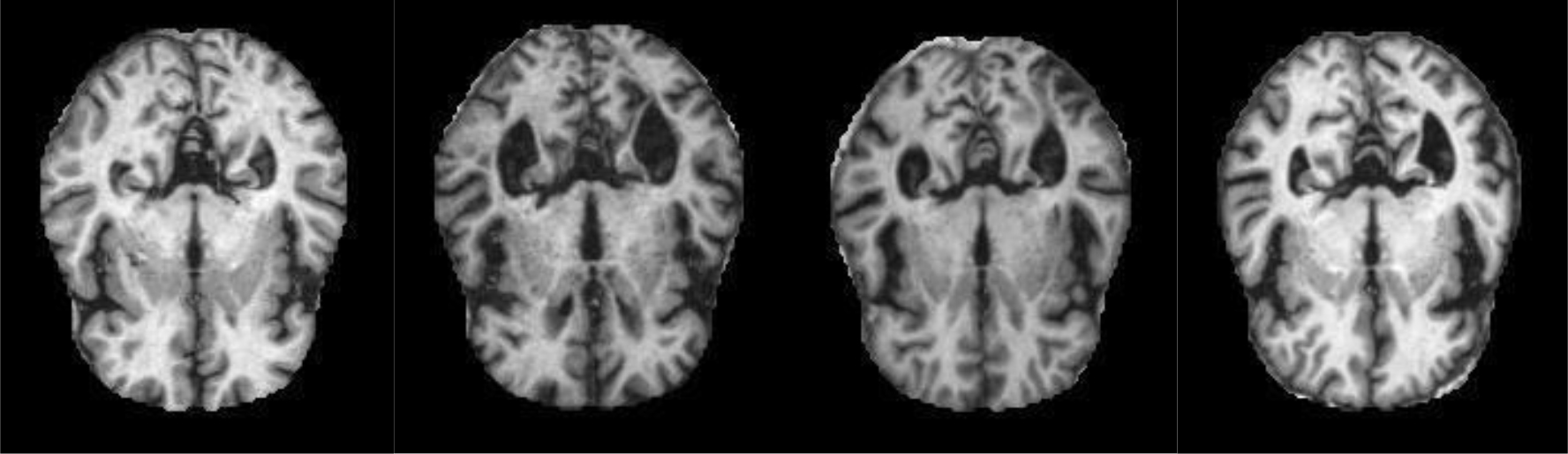

Figure 8.
Non-Demented images.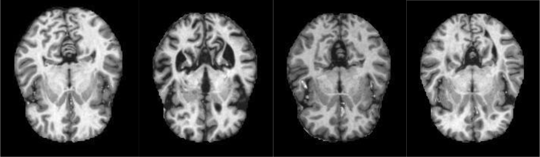

Another important parameter is gamma, which is the kernel coefficient. “scale” is the default value for gamma.

3.5 Performance evaluation

Index	Model name	Accuracy	Precision	Recall	F1-score
1	Logistic Regression	0.946429	0.983051	0.920635	0.95082
2	LR-Hyper parameter Tuning	0.946429	0.983051	0.920635	0.95082
3	Naive Bayes	0.955357	0.983051	0.935484	0.958678
4	KNN	0.928571	0.932203	0.932203	0.932203
5	KNN-Hyper parameter Tuning	0.839286	0.864407	0.836066	0.85
6	Random Forest	0.928571	0.949153	0.918033	0.933333
7	RF-Hyper parameter Tuning	0.919643	0.932203	0.916667	0.92437
8	ADA Boost	0.928571	0.966102	0.904762	0.934426
9	ADA Boost-Hyper parameter Tuning	0.946429	0.983051	0.920635	0.95082
10	Gradient Boosting	0.866071	0.813559	0.923077	0.864865
11	GB-Hyper parameter Tuning	0.9375	0.966102	0.919355	0.942149
12	XG Boost	0.901786	0.881356	0.928571	0.904348
13	XGB-Hyper parameter Tuning	0.946429	0.983051	0.920635	0.95082
14	SVM	0.946429	0.983051	0.920635	0.95082
15	SVM-Hyper parameter Tuning	0.946429	0.983051	0.920635	0.95082

Performance of different ML algorithms were evaluated in terms of Accuracy, Precision, Recall and F1 Score. Table 2 depicts the performance parameter values of each model.

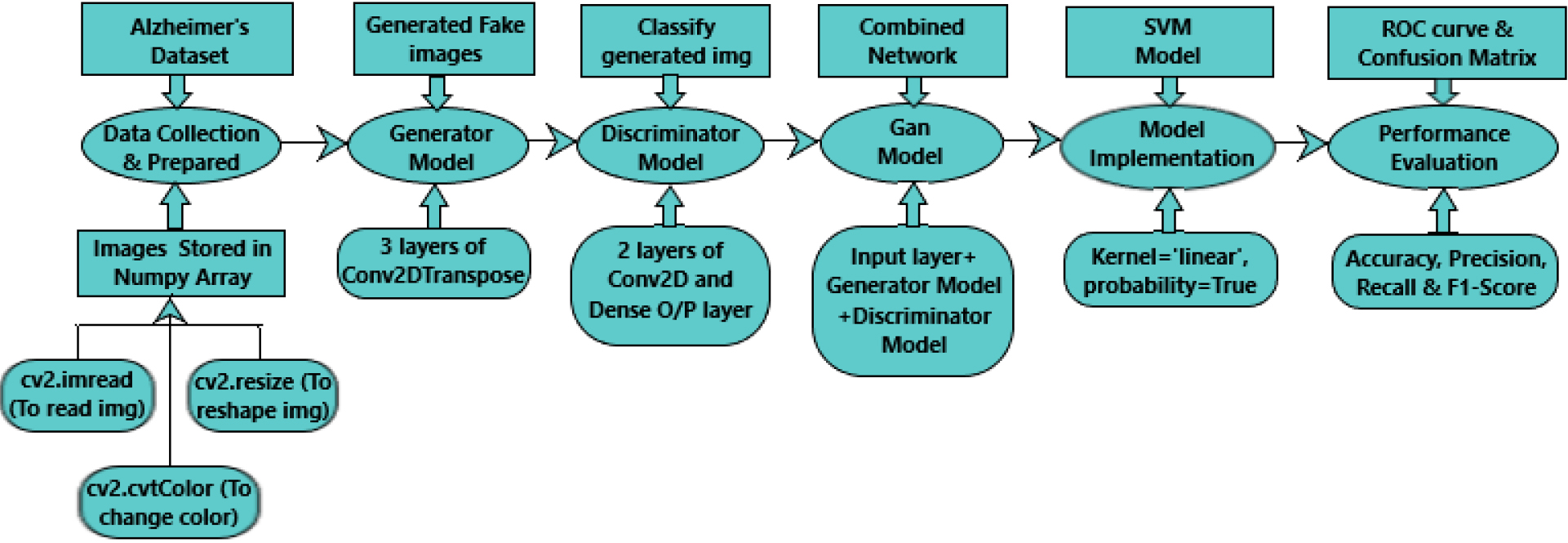
4. Proposed methodology 2 (image dataset)

In method II, Alzheimer’s MRI dataset was used. This involved: Data Collection and Data Preparation, Generator Model, Discriminator Model, Gan Model, Model Implementation and Performance Evaluation using Alzheimer’s dataset (4 class of images). Each Procedure is explained in further sections. Figure 6 depicts the Proposed method II.

Figure 9.

Generated images.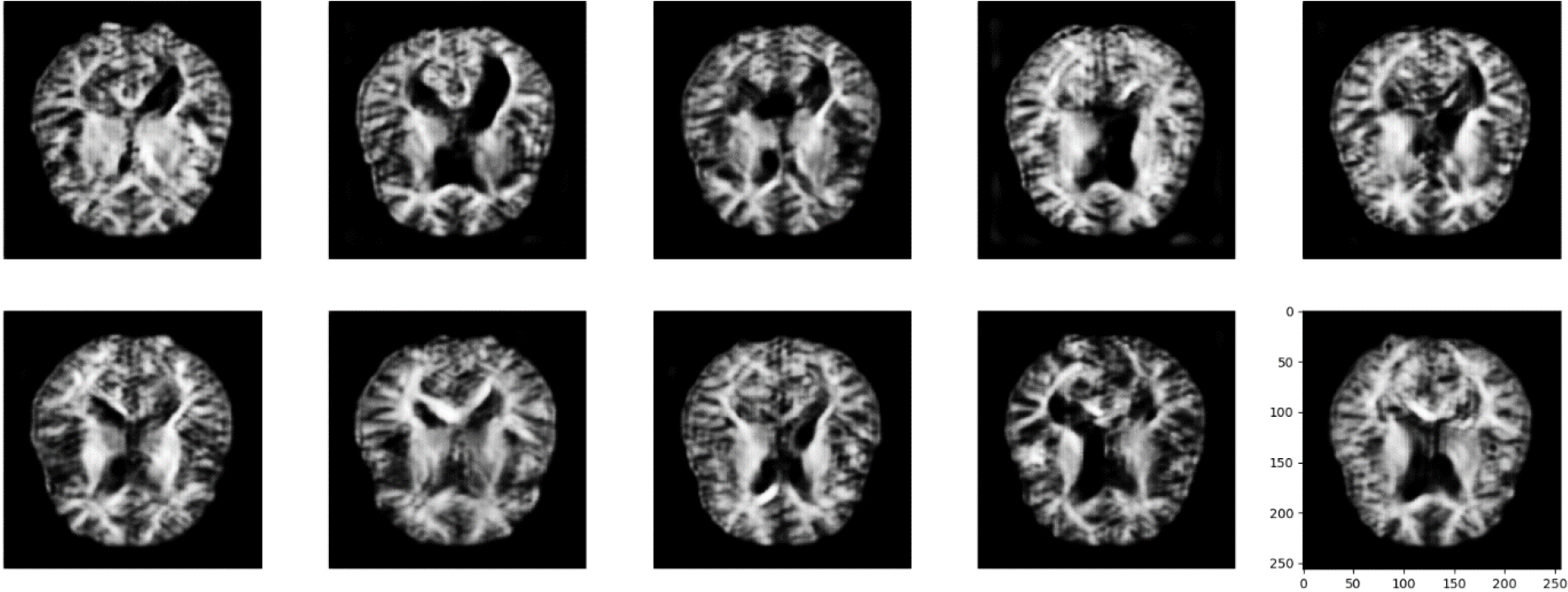

Figure 10.

ROC curve for LR.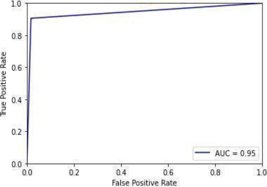

Figure 11.

Confusion Matrix of LR.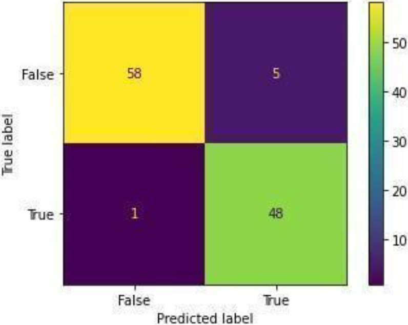

Figure 12.

ROC curve for LR-HT.

Figure 13.

Confusion Matrix of LR-HT.

Figure 14.

ROC curve for NB.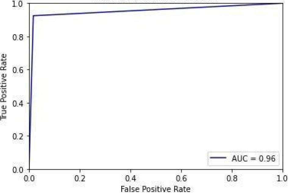

Figure 15.

Confusion Matrix of NB.

4.1 Data collection and data preparation

Alzheimer’s dataset (4 class of images) available on Kaggle is used. The dataset consists of a total of 6400 images in training as well as test directory. It has MRI images divided into four classes of images-patients having Mild Dementia, Moderate Dementia, No Dementia and Very Mild Dementia. In the train directory, there are 717 files for Mild demented patients, 52 files of Moderate Demented patients and 2560 files of non-Demented patients and 1792 files of Very Mild Demented patients. In the test directory, there are 179 files of Mild demented patients, 12 files of Moderate Demented patients, 640 files of non-Demented patients, 448 files of Very Mild Demented patients. Figure 7 shows the mild demented MRI images and Fig. 8 shows the Non-demented MRI images. In this work, only these two classes are considered to train the model.

To prepare these images for training, the first step is to read these images from the directory with the help of cv2.imread() function. After that color of these images are converted to gray with the help of cv2.cvtColor() function. It is important to reshape all the images into fixed width and height before training. So, the last step of data preparation is to reshape all the images with the help of cv2.resize() function.

All these prepared images are then stored in NumPy array with the help of np. array () function.

4.2 Generator model

Figure 16.

ROC curve for KNN.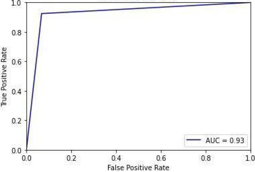

Figure 17.

Confusion Matrix of KNN.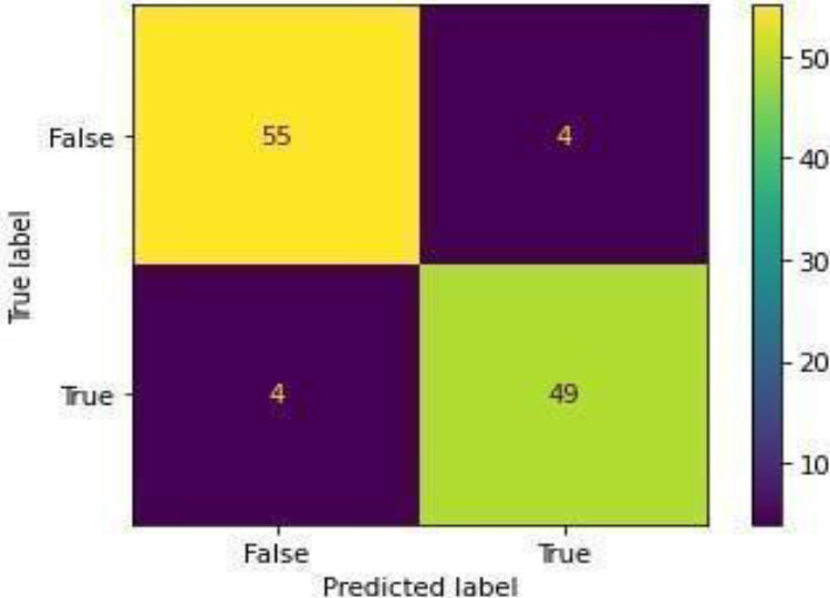

Figure 18.

ROC curve for KNN-HT.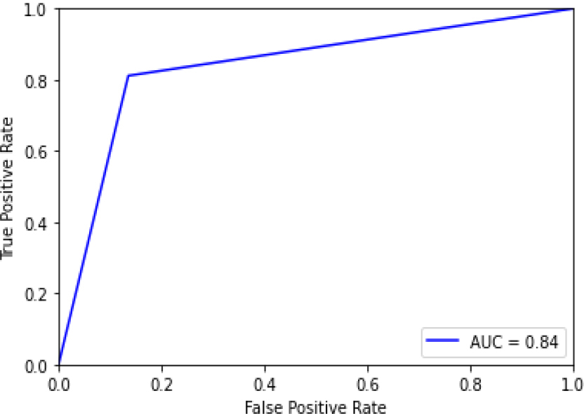

Figure 19.

Confusion Matrix of KNN-HT.

Figure 20.

ROC curve for RF.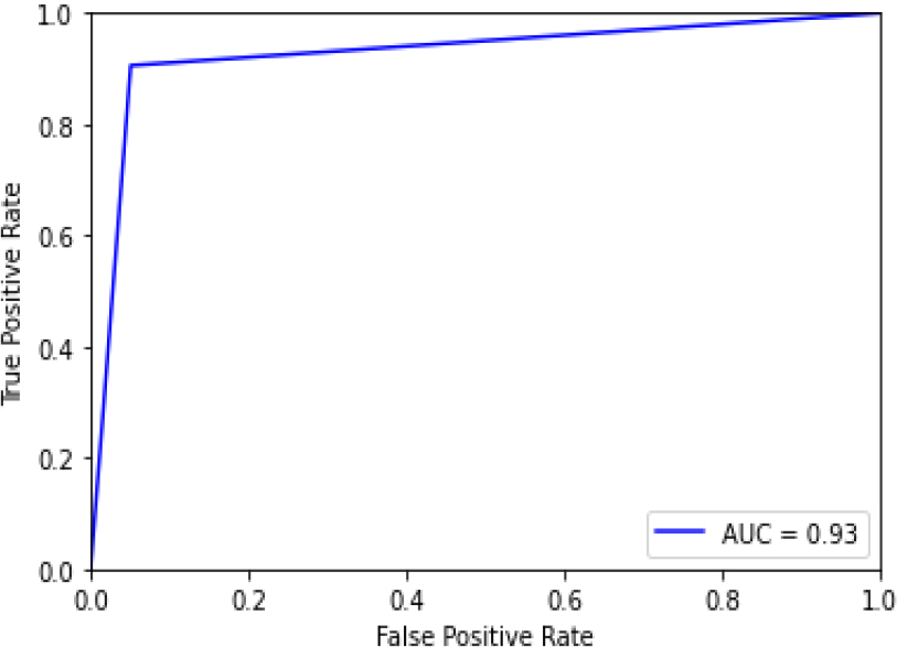

Figure 21.

Confusion Matrix of RF.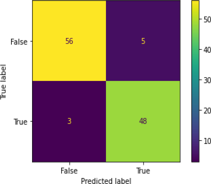

Figure 22.

ROC curve for RF-HT.

Figure 23.

Confusion Matrix of RF-HT.

Figure 24.

ROC curve for ADB.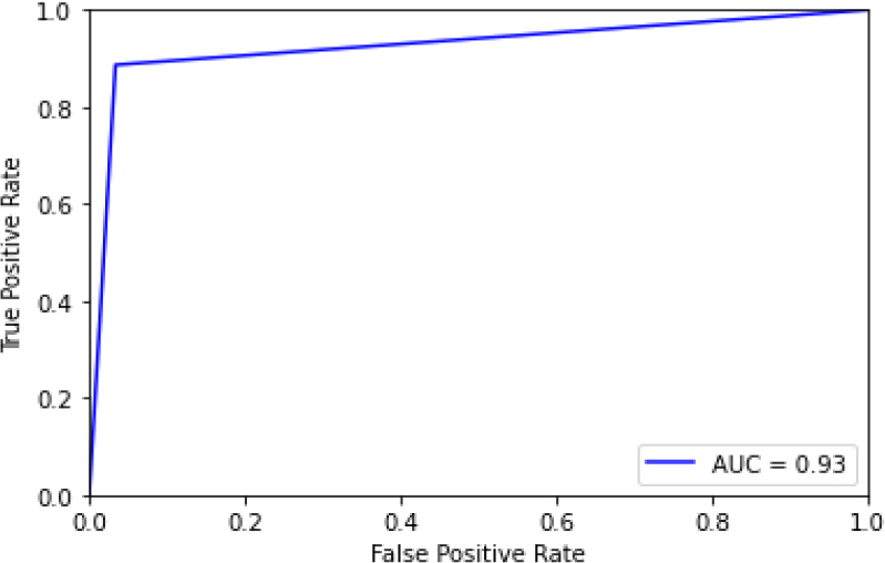

Figure 25.

Confusion Matrix of ADB.

Figure 26.

ROC curve for ADB-HT.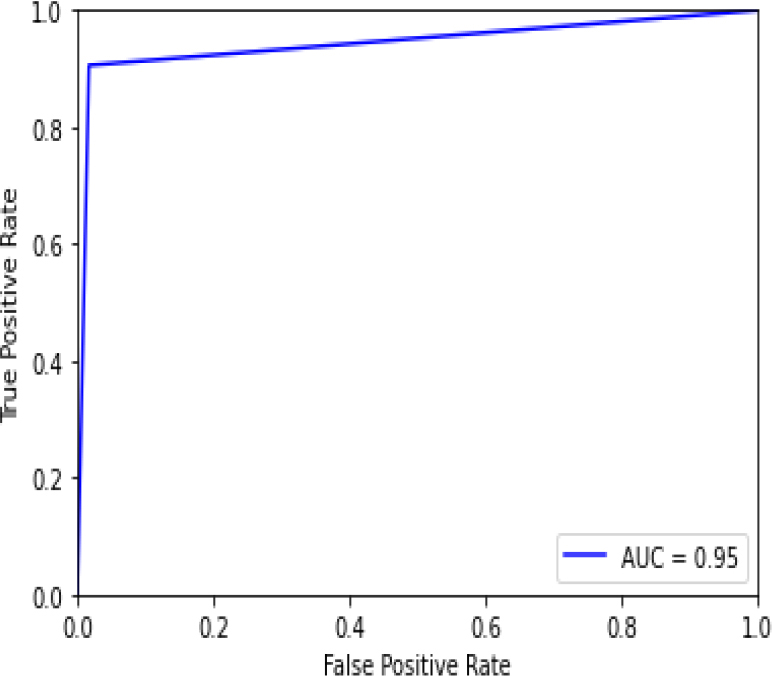

Alzheimer’s dataset (4 class of images) is unbalanced and to train the model balanced data is needed. So, to balance this dataset generator model is used. Generator models generate fake images from the existing ones by adding random noise in images. The random noise sampled with latent vector is given as input to the generator model. The generator model then produced a transformed image using transposed convolutional. 3 layers of Conv2DTranspose layers are used. 10 times generator model transposes the images 10 times and 50 Epochs run at every time. Output images of the last step were given as input to the next step. So, at the last step generator model produces images which are shown in Fig. 9.

Figure 27.

Confusion Matrix of ADB-HT.

Figure 28.

ROC curve for GB.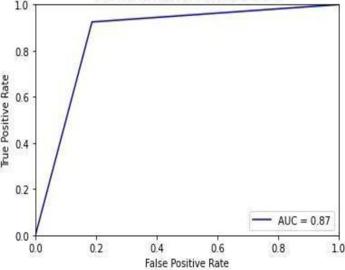

4.3 Discriminator model

Discriminator is the model which manages classifying the generated images as fake or real. The goal is to create a Generator so powerful that the Discriminator is unable to classify real and fake images. 2 Conv2D layers connected to a Dense output layer is used.

4.4 Gan model

Gan stands for Generative Adversarial Network model. In this work, the gan model is a combination of input layer, generator model and discriminator model. Basically, it is a combined network.

4.5 Model implementation

Support vector machine (SVM) Model is trained. Kernel is set as ‘linear’, and probability is True.

4.6 Performance evaluation

After model training, the performance of SVM model is evaluated. SVM model achieves 0.84493 accuracy, 0.917209 precision, 0.64525 recall and 0.67997 F1 score.

5. Result and discussions

ROC curve and Confusion matrix of all models are discussed in this section.

Figure 10 shows the ROC curve for the logistic regression, showing 0.95 accuracy. Figure 11 shows the confusion matrix for the logistic regression, showing that 6 predictions were false, and 106 predictions were true.

Figure 12 is the ROC curve of the logistic regression – hyperparameter tuning shows that the accuracy is 0.95. Figure 13 shows the confusion matrix for logistic regression – hyperparameters showing 6 predictions as false and 106 predictions as true.

Figure 14 shows the ROC curve for Naive Bayes with 0.96 accuracy. Figure 15 shows the confusion matrix for Naive Bayes, showing that 5 predictions were false, and 107 predictions were true.

Figure 16 shows the ROC curve for KNN with an accuracy of 0.93. Figure 17 shows the confusion matrix for KNN, showing that 8 predictions were false, and 104 predictions were true.

Figure 18 shows the ROC curve for KNN – hyperparameter tuning shows an accuracy of 0.84. Figure 19 shows the confusion matrix for KNN – hyperparameter parameters showing 18 predictions as false and 94 as true.

Figure 29.

Confusion Matrix of GB.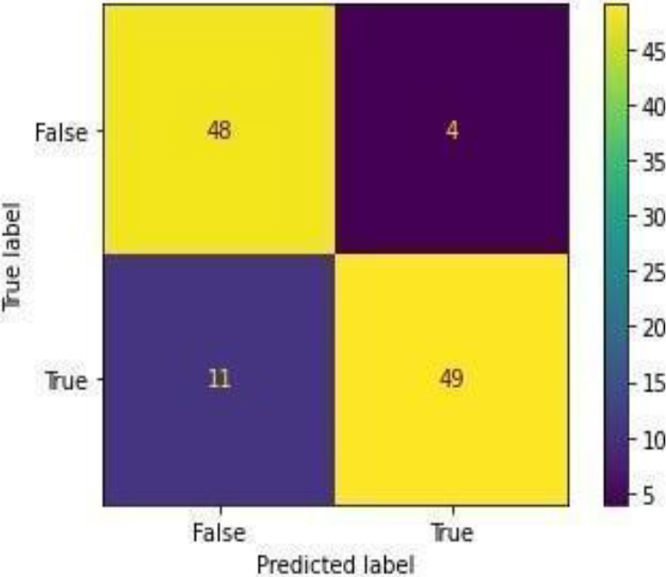

Figure 30.

ROC curve for GB-HT.

Figure 31.

Confusion Matrix of GB-HT.

Figure 32.

ROC curve for XGB.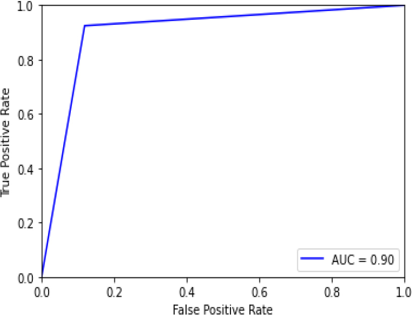

Figure 33.

Confusion Matrix of XGB.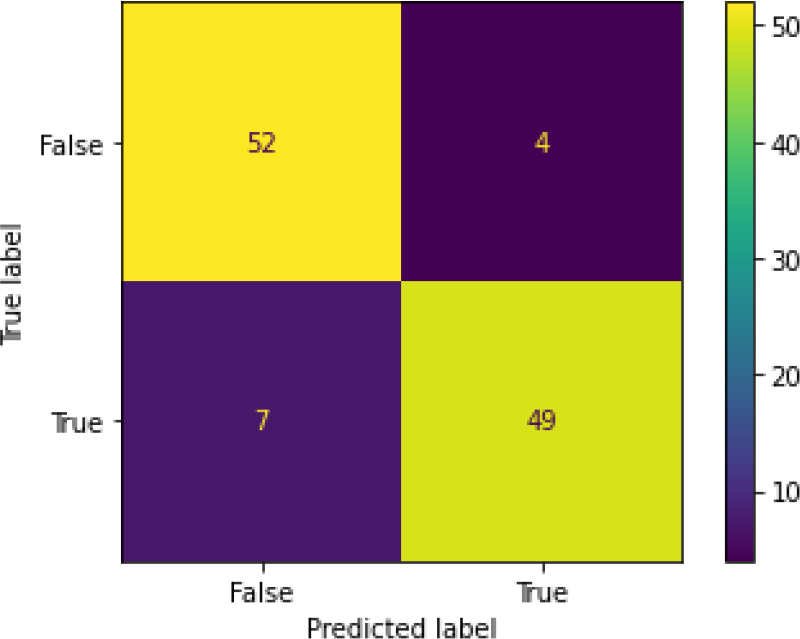

Figure 34.

ROC curve for XGB-HT.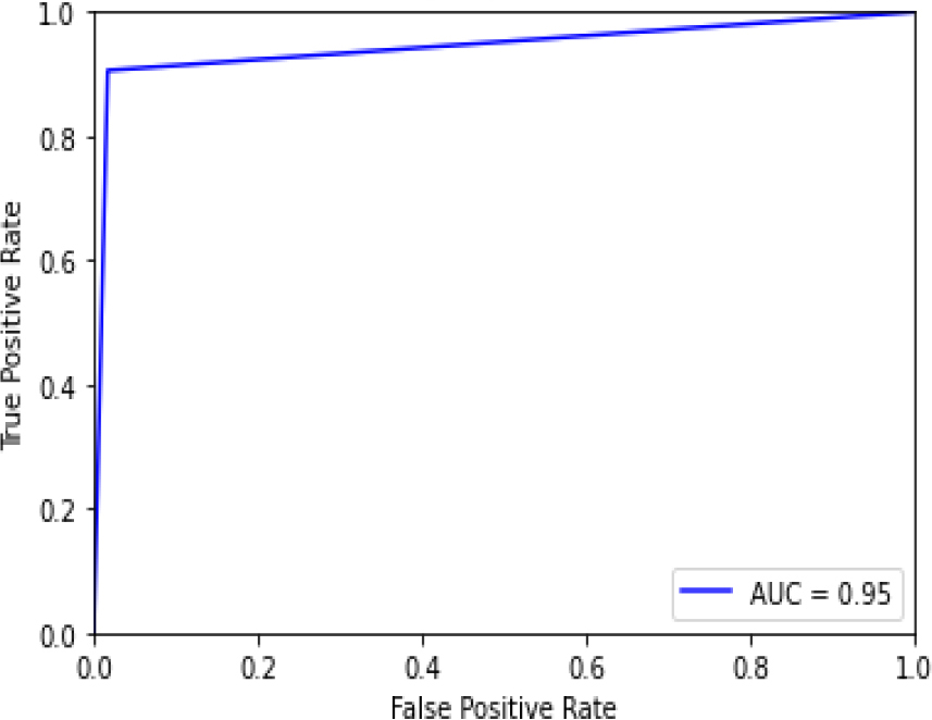

Figure 35.

Confusion Matrix of XGB-HT.

Figure 36.

ROC curve for SVM.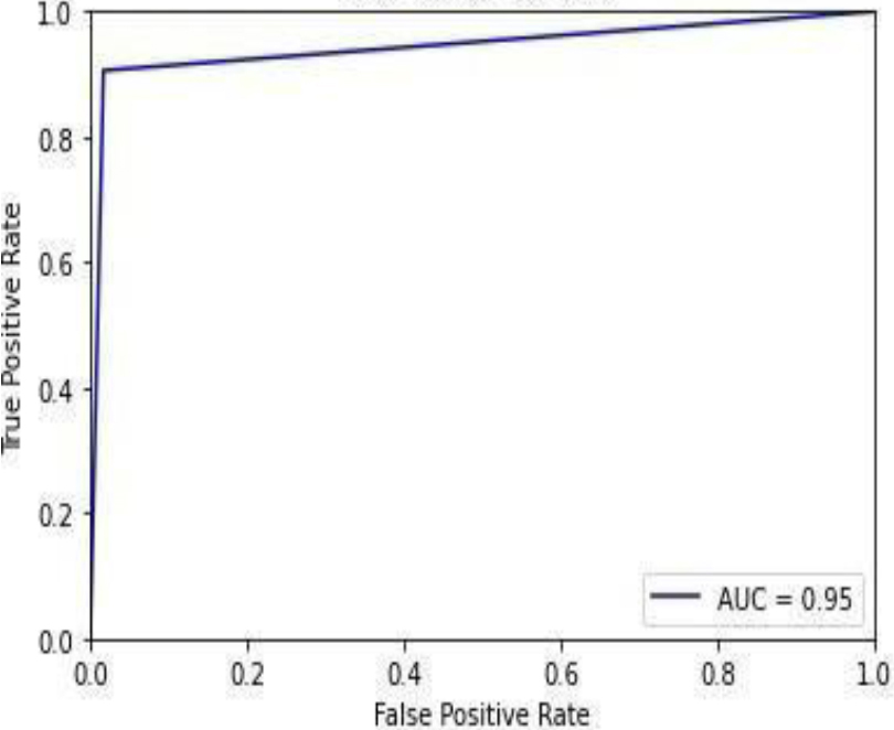

Figure 37.

Confusion Matrix of SVM.

Figure 38.

ROC curve for SVM-HT.

Figure 20 shows the ROC curve for Random Forest with an accuracy of 0.93. Figure 21 shows the confusion matrix for Random Forest, showing that 8 predictions were false, and 104 predictions were true.

Figure 22 shows the ROC curve for random forest – hyperparameter tuning shows an accuracy of 0.92. Figure 23 shows the confusion matrix for Random Forest – hyperparameter parameters showing 9 predictions as false and 103 as true.

Figure 24 shows the ROC curve for ADA Boost, showing an accuracy of 0.93. Figure 25 shows the confusion matrix for ADA Boost, showing that 8 predictions were false, and 104 predictions were true.

Figure 26 shows the ROC curve for ADA Boost – the hyperparameter tuning showing an accuracy of 0.95. Figure 27 shows the confusion matrix for ADA Boost – hyperparameter tuning, showing 6 predictions as false and 106 as true.

Figure 28 shows the ROC curve for the gradient boost, showing an accuracy of 0.87. Figure 29 shows the confusion matrix for the gradient boost, showing that 15 predictions were false, and 97 predictions were true.

Figure 30 shows the ROC curve for Gradient Boosting – hyperparameter tuning shows an accuracy of 0.87. Figure 31 shows the confusion matrix for the gradient boost – hyperparameter parameters showing 15 predictions as false and 97 as true.

Figure 32 shows the ROC curve for XGBoost, showing an accuracy of 0.90. Figure 33 shows the confusion matrix for XG Boost, showing that 11 predictions were false, and 101 predictions were true.

Figure 34 shows the ROC curve of XG Boost – Hyper Parameter Tuning, and the display accuracy is 0.95. Figure 35 shows the confusion matrix for XGBoost – hyperparameter tuning, showing 6 predictions as false and 106 as true.

Figure 36 shows the ROC curve of the SVM with an accuracy of 0.95. Figure 37 shows the confusion matrix for the SVM, showing that 6 predictions were false, and 106 predictions were true.

Figure 39.

Confusion Matrix of SVM-HT.

Figure 40.

ROC AUC Curve of different ML algorithms.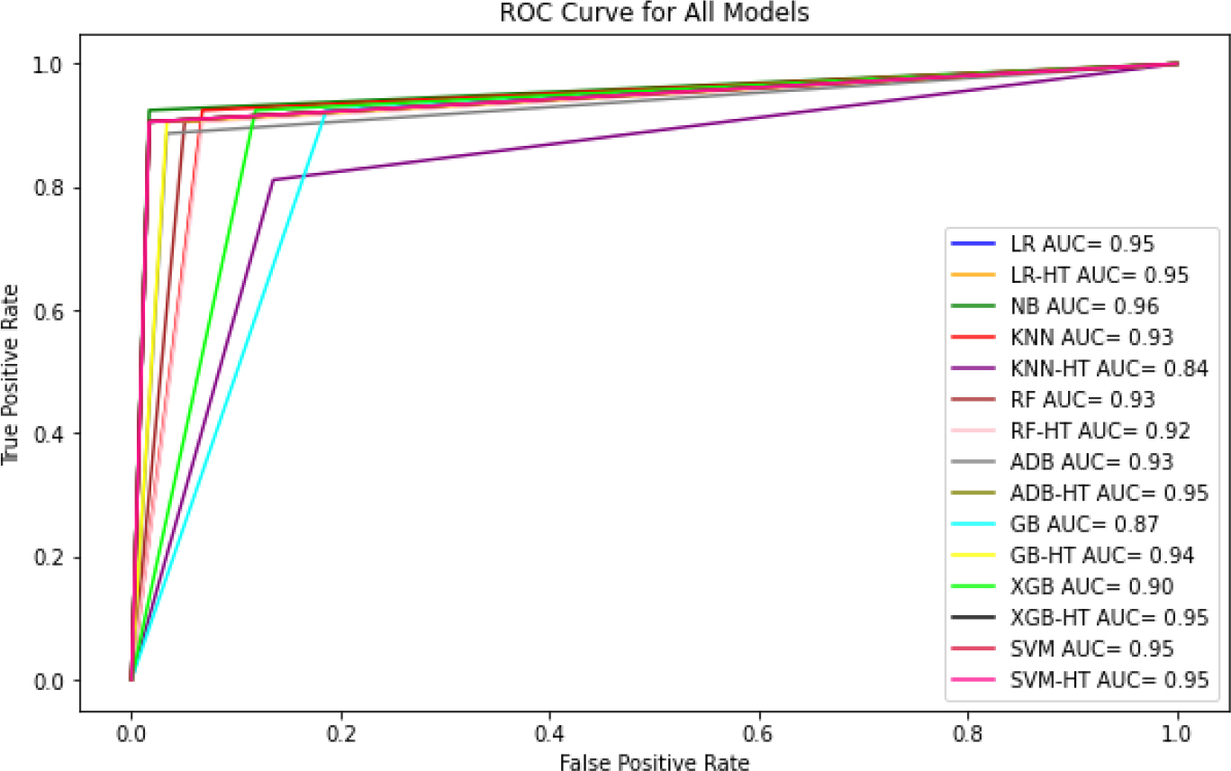

Figure 41.

ROC curve for SVM (Image).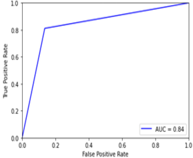

Figure 42.

Confusion Matrix of SVM (Image).

Figure 38 shows the ROC curve for the SVM – hyperparameter tuning shows an accuracy of 0.95. Figure 39 shows the confusion matrix for the SVM – hyperparameter parameters showing 6 predictions which were false and 106 predictions which were true.

Figure 40 shows the ROC curve of different ML algorithms in which the blue line shows the ROC curve for Logistic Regression which has 0.95% accuracy. Orange line is the LR-Hyper parameter tuning ROC curve with 0.95% accuracy. Green line depicts the Naïve Bayes ROC curve resulting in 0.96% accuracy. Red line shows the KNN ROC curve with 0.93% accuracy. Purple line shows the KNN-Hyper parameter tuning ROC curve giving 0.84% accuracy. Brown line is the Random Forest ROC curve with 0.92% accuracy. The pink line shows the RF-Hyper parameter Tuning ROC curve resulting in 0.92% accuracy. Gray line shows the ADABoost ROC curve with 0.93% accuracy. The olive line shows the ADB-Hyper parameter Tuning ROC curve with 0.95% accuracy. Cyan line shows the Gradient Boosting ROC curve with 0.87% accuracy. The yellow line shows the GB-Hyper parameter Tuning ROC curve with 0.94% accuracy. Lime line shows the XG Boost ROC curve with 0.90% accuracy. Black line shows the XGB-Hyper parameter tuning ROC curve providing 0.95% accuracy. The Crimson line shows the SVM ROC curve with 0.95% accuracy. The Deep Pink line shows the SVM-Hyper parameter tuning ROC curve with 0.95% accuracy.

Naïve Bayes is the best among all because it gives a more correct value with the accuracy of 0.955357. Naïve Bayes has 0.983051 precision value, 0.935484 recall and 0.958678 F1-score.

Figure 41 Shows the ROC curve for SVM Model for image dataset which has 84.4% accuracy. It achieves less accuracy as compared to other models which are trained on numeric datasets. Figure 42 shows the confusion matrix of SVM model which is trained on image dataset. SVM model predicts 94 true values and 18 false values.

6. Conclusion and future work

OASIS – longitudinal Dataset from Kaggle which has 373 rows and 15 columns numeric values and Alzheimer’s dataset (4 class of images) from Kaggle which contains 6400 images of MRI segments is used. Most correlated features were selected from OASIS dataset by mutual information classification method. It was seen that CDR had a high correlation with the target variable. 6 most correlated features were selected to avoid overfitting. On the other side, Generator model is built to generate fake images to balance the Alzheimer’s dataset. Logistic regression, LR-Hyper parameter Tuning, Naïve Bayes, K-Nearest Neighbor, KNN-Hyper parameter Tuning, Random Forest, RF – Hyper parameter Tuning, ADA Boost, ADB-Hyper parameter Tuning, Gradient Boosting, GB – Hyper parameter Tuning, XGBoost, XGB-Hyper parameter Tuning, SVM and SVM – Hyper parameter Tuning algorithms were trained on OASIS dataset. The results for OASIS data are shown in Table 2 and it can be concluded that Naïve Bayes is the best among all as it has the highest accuracy of 0.955357. SVM model was trained using Alzheimer’s image dataset. It can be concluded that SVM model achieves less accuracy on image dataset as compared to the models trained on OASIS numeric dataset. In future, performance of deep learning algorithms with image dataset can be evaluated to provide better Automated diagnosis solutions. Also Ensemble learning approach can be explored to improve the accuracy in early diagnosis of Dementia disease.

Footnotes

Statements and declarations

Competing Interests: The authors have no competing interests to declare that are relevant to the content of this article.

Funding Interests: The authors did not receive support from any organization for the submitted work.

Financial interests: The authors declare they have no financial interests.

References

Khan

Zubair

. Expansion of Regularized K means Discretization Machine Learning Approach in Prognosis of Dementia Progression. Proceedings of the 2020 11th International Conference on Computing, communication, and Networking Technologies (ICCCNT), 2020 July 1–3; Kharagpur, India; 2020, pp. 1-6, doi: 10.1109/ICCCNT49239.2020.9225397.

Herzog

Magoulas

. Brain Asymmetry Detection and Machine Learning Classification for Diagnosis of Early Dementia. Sensors (Basel). 2021 Jan 24; 21(3): 778; PMID: 33498908; PMCID: PMC7865614; doi: 10.3390/s21030778.

Tsang

Xie

Zhou

. Harnessing the Power of Machine Learning in Dementia Informatics Research: Issues, Opportunities, and Challenges. IEEE Rev Biomed Eng. 2020; 13: 113-129. Epub 2019 Mar 12. PMID: 30872241. doi: 10.1109/RBME.2019.2904488.

Arevalo-Rodriguez

Smailagic

Roqué-Figuls

Ciapponi

Sanchez-Perez

Giannakou

et al. Mini-Mental State Examination (MMSE) for the early detection of dementia in people with mild cognitive impairment (MCI). Cochrane Database of Systematic Reviews. 2021 July 27 Issue 7. Art. No.: CD010783. doi: 10.1002/14651858.CD010783.pub3.

Ullah

. M.

Onik

Islam

Nandi

. Alzheimer’s Disease and Dementia Detection from 3D Brain MRI Data Using Deep Convolutional Neural Networks. Proceedings of the 2018 3rd International Conference for Convergence in Technology (I2CT), 2018 April 6–8; Pune, India; 2018, pp. 1-3. doi: 10.1109/I2CT.2018.8529808.

Bansal

Chhikara

Khanna

Gupta

. Comparative Analysis of Various Machine Learning Algorithms for Detecting Dementia. Procedia Computer Science. 2018 Volume 132, Pages 1497-1502. ISSN 1877-0509, doi: 10.1016/j.procs.2018.05.102.

Battineni

Chintalapudi

Amenta

. Machine learning in medicine: Performance calculation of dementia prediction by support vector machines (SVM). Informatics in Medicine Unlocked. 2019; Volume 16: 10020. ISSN 2352-9148. doi: 10.1016/j.imu.2019.100200.

Bidani

Gouider

Travieso

. Dementia Detection and Classification from MRI Images Using Deep Neural Networks and Transfer Learning Proceedings Part I of the 15th International Work-Conference on Artificial Neural Networks, IWANN 2019 June 12–14; Gran Canaria, Spain; 2019. doi: 10.1007/978-3-030-20521-8_75.

Guram

Sharma

. Comparing the Performance of Various Machine Learning Approaches in Identifying Different Classes of Dementia. Proceedings of the International Conference on Innovative Computing & Communication (ICICC) 2021; p. 9. doi: 10.2139/ssrn.3833832.

10.

Faouri

AlBashayreh

Azzeh

. Examining stability of machine learning methods for predicting dementia at early phases of the disease. Decision Science Letters. 2022; pp. 333-346. doi: 10.5267/j.dsl.2022.1.005.

11.

Kour

Manhas

Sharma

. Comparative Study of Different Machine Learning Techniques in the Diagnosis of Dementia. Advances in Intelligent Systems and Computing. 2020; Vol. 1187: pp. 93-104. doi: 10.1007/978-981-15-6014-9_12.

12.

Byeon

. Screening dementia and predicting high dementia risk groups using machine learning. World Journal of Psychiatry. 2022; vol. 12(2): pp. 204-211. PMID: 35317343, PMCID: PMC8900592. doi: 10.5498/wjp.v12.i2.204.

13.

Veeralagan

Priya

. Hyper Tuning Using Gridsearchcv on Machine Learning Models for Prognosticating Dementia. Research Square. 2022. doi: 10.21203/rs.3.rs-2316713/v1.

14.

Zhang

Petersen

Johnson

Hall

O’Bryant

. Accelerating Hyperparameter Tuning in Machine Learning for Alzheimer’s Disease with High Performance Computing. Frontiers in Artificial Intelligence. 2021; vol. 4. doi: 10.3389/frai.2021.798962.

15.

Basheer

Bhatia

Sakri

. Computational Modeling of Dementia Prediction Using Deep Neural Network: Analysis on OASIS Dataset. IEEE Access. 2021; vol. 9, pp. 42449-42462. doi: 10.1109/access.2021.3066213.

16.

Sørensen

Nielsen

. Ensemble support vector machine classification of dementia using structural MRI and mini-mental state examination. Journal of Neuroscience Methods. 2018; vol. 302. pp. 66-74. doi: 10.1016/j.jneumeth.2018.01.003.

17.

Math Kunti

Rangaswamy

. Machine Learning Techniques to Identify Dementia. SN Computer Science. 2020; vol. 1(3). doi: 10.1007/s42979-020-0099-4.

18.

James

Ranson

Everson

Llewellyn

. Performance of Machine Learning Algorithms for Predicting Progression to Dementia in Memory Clinic Patients. JAMA Network Open. Dec. 2021; vol. 4(12). doi: 10.1001/jamanetworkopen.2021.36553.

19.

Rawat

Akram

Mithil Pradeep

. Dementia Detection Using Machine Learning by Stacking Models. Proceedings of the 2020 5th International Conference on Communication and Electronics Systems (ICCES),2020; Coimbatore, India; 2020, pp. 849-854. doi: 10.1109/ICCES48766.2020.9137852.

20.

Neelaveni

Devasana

. Alzheimer Disease Prediction using Machine Learning Algorithms. Proceedings of the 6th International Conference on Advanced Computing and Communication Systems (ICACCS), Mar. 2020; pp. 101-104. doi: 10.1109/icaccs48705.2020.9074248.

21.

Kavitha

Mani

Srividhya

Khalaf

Romero

CAT

. Early-Stage Alzheimer’s Disease Prediction Using Machine Learning Models. Frontiers in public health. 2022; PMID: 35309200, PMCID: PMC8927715, doi: 10.3389/fpubh.2022.853294.

22.

Kim

Lim

. A Deep Neural Network-Based Method for Prediction of Dementia Using Big Data. International Journal of Environmental Research and Public Health. 2021; vol. 18(10): p. 5386. doi: 10.3390/ijerph18105386.

23.

Zhu

Tang

Zhang

Hung

et al. Machine Learning for the Preliminary Diagnosis of Dementia. Scientific Programming. 2020; vol. 2020: pp. 1-10. doi: 10.1155/2020/5629090.

24.

Arifoglu

Bouchachia

. Detection of abnormal behavior for dementia sufferers using Convolutional Neural Networks. Artificial Intelligence in Medicine. 2019; vol. 94: pp. 88-95. doi: 10.1016/j.artmed.2019.01.005.

25.

Danso

Zeng

Muniz-Terrera

Ritchie

. Developing an Explainable Machine Learning-Based Personalized Dementia Risk Prediction Model: A Transfer Learning Approach with Ensemble Learning Algorithms. Frontiers in Big Data. 2021; vol. 4. doi: 10.3389/fdata.2021.613047.

26.

Vinayak

, A S Khan

. Dementia Prediction on OASIS Dataset using Supervised and Ensemble Learning Techniques. International Journal of Engineering and Advanced Technology. 2020; 10(1): pp. 244-254. doi: 10.35940/ijeat.a1827.1010120.

27.

Antor

Jamil

AHMS

Mamtaz

Khan

Aljahdali

Kaur

et al. A Comparative Analysis of Machine Learning Algorithms to Predict Alzheimer’s Disease. Journal of Healthcare Engineering. 2021; vol. 2021: pp. 1-12. doi: 10.1155/2021/9917919.

28.

Ali

Islam

Haque

Das

Duranta

Islam

. Alzheimer’s Disease Detection Using m-Random Forest Algorithm with Optimum Features Extraction. Proceedings of the 2021 1st International Conference on Artificial Intelligence and Data Analytics (CAIDA). April 6-7, 2021; Riyadh, Saudi Arabia. doi: 10.1109/caida51941.2021.9425212.

29.

Battineni

Hossain

Chintalaoudi

Traini

Dhulipalla

Ramasamy

et al. Improved Alzheimer’s Disease Detection by MRI Using Multimodal Machine Learning Algorithms. Diagnostics. 2021; vol. 11(11): p. 2103. doi: 10.3390/diagnostics11112103.

30.

Vuong

Chan

Lau

. Conceptual map and technological framework to manage dementia wandering. Proceedings of the 2014 IEEE International Symposium on Bioelectronics and Bioinformatics (IEEE ISBB 2014), May 11-14 2014; Chungli Taiwan; 2014. doi: 10.1109/isbb.2014.6820889.

31.

Miah

Prima

CNE

Seema

Mahmud

Kaiser

. Performance Comparison of Machine Learning Techniques in Identifying Dementia from Open Access Clinical Datasets. Advances in Intelligent Systems and Computing. 2020; pp. 79-89. doi: 10.1007/978-981-15-6048-4_8.

32.

Zhang

Petersen

Johnson

Hall

O’Bryant

. Accelerating Hyperparameter Tuning in Machine Learning for Alzheimer’s Disease with High Performance Computing. Frontiers in Artificial Intelligence. 2021; vol. 4. doi: 10.3389/frai.2021.798962.

33.

Yuan

Bian

Cai

Huang

Church

. Disfluencies and Fine-Tuning Pre-Trained Language Models for Detection of Alzheimer’s Disease. Interspeech. 2020. doi: 10.21437/interspeech.2020-2516.

34.

Herzog

Magoulas

. Brain Asymmetry Detection and Machine Learning Classification for Diagnosis of Early Dementia. Sensors. 2021; vol. 21(3): p. 778. doi: 10.3390/s21030778.

35.

Spooner

Chen

Sowmya

Sachdev

Kochan

Trollor

et al. A comparison of machine learning methods for survival analysis of high-dimensional clinical data for dementia prediction. Scientific Reports. 2020; vol. 10(1). doi: 10.1038/s41598-020-77220-w.

36.

Naganandhini

Shanmugavadivu

. Effective Diagnosis of Alzheimer’s Disease using Modified Decision Tree Classifier. Procedia Computer Science. 2019; vol. 165, pp. 548-555. doi: 10.1016/j.procs.2020.01.049.

37.

Javeed

Dallora

Berglund

Anderberg

. An Intelligent Learning System for Unbiased Prediction of Dementia Based on Autoencoder and ADAboost Ensemble Learning. Life. 2022; vol. 12(7): p. 1097. doi: 10.3390/life12071097.

38.

Kleiman

Barenholtz

Galvin

. Screening for early-stage Alzheimer’s disease using optimized feature sets and machine learning. J Alzheimers Disease. 2021; 81(1): 355-366. PMID: 33780367; PMCID: PMC8324324. doi: 10.3233/JAD-201377.

39.

Wang

Hou

Zhang

Cao

. Construction of a risk prediction model for Alzheimer’s disease in the elderly population. BMC Neurology. 2021; vol. 21(1). doi: 10.1186/s12883-021-02276-8.

40.

Fukunishi

Nishiyama

Luo

Kubo

Kobayashi

. Alzheimer-type dementia prediction by sparse logistic regression using claim data. Computer Methods and Programs in Biomedicine. 2020 Nov; 196: p. 105582. doi: 10.1016/j.cmpb.2020.105582.

41.

Vuong

Chan

Lau

. Automated detection of wandering patterns in people with dementia. Gerontechnology. 2014; vol. 12(3). doi: 10.4017/gt.2014.12.3.001.00.

42.

Bhagya Shree

Sheshadri

. Diagnosis of Alzheimer’s disease using Naïve Bayesian Classifier. Neural Computer & Application. 2018; 29: 123-132. doi: 10.1007/s00521-016-2416-3.

43.

Balamurugan

Nancy

Vijaykumar

. Alzheimer’s Disease Diagnosis by using Dimensionality Reduction Based on KNN Classifier. Biomedical and Pharmacology Journal. 2017; vol. 10(4): pp. 1823-1830. doi: 10.13005/bpj/1299.

44.

Vyas

Aisopos

Vidal

Garrard

Paliouras

. Identifying the Presence and Severity of Dementia by Applying Interpretable Machine Learning Techniques on Structured Clinical Records. BMC Medical Informatics and Decision Making. 2022; article 271. doi: 10.21203/rs.3.rs-336921/v1.

45.

Sarica

Cerasa

Quattrone

. Random Forest Algorithm for the Classification of Neuroimaging Data in Alzheimer’s Disease: A Systematic Review. Front Aging Neurosci. 2017 Oct 6; 9: 329. PMID: 29056906; PMCID: PMC5635046. doi: 10.3389/fnagi.2017.00329.

46.

Javeed

Dallora

Berglund

Anderberg

. An Intelligent Learning System for Unbiased Prediction of Dementia Based on Autoencoder and ADAboost Ensemble Learning. Life. 2022; vol. 12(7): p. 1097. doi: 10.3390/life.12071097.

47.

Abarna

Pranesha

Fathima

Priyadharshini

Karthikeyan

. Detection of Alzheimer’s disease using gradient boosting algorithm. International Research Journal of Engineering and Technology. 2020; vol. 07, issue 09. e-ISSN: 2395-0056, P-ISSN 2395-0072. https//www.irjet.net/archives/V7/i9/IRJET-V7I9443.pdf.

48.

Shojaie

Cabrerizo

DeKosky

Loewenstein

Duara

Ajouadi

. A transfer learning approach based on gradient boosting machine for diagnosis of Alzheimer’s disease. Frontiers in Aging Neuroscience. 2022; vol. 14. doi: 10.3389/fnagi.2022.966883.

49.

Ryu

Shin

Chung

. Prediction Model of Dementia Risk Based on XGBoost Using Derived Variable Extraction and Hyper Parameter Optimization. IEEE Access. 2020; vol. 8: pp. 177708-177720. doi: 10.1109/access.2020.3025553.

50.

Tanveer

Richhariya

Khan

Rashid

Khanna

Prasad

Lin

. Machine Learning Techniques for the Diagnosis of Alzheimer’s Disease: A Review. ACM Trans. Multimedia Comput. Communication Applications. 2020; 16(1): Article 30, pp. 1-35. doi: 10.1145/3344998.

51.

Sharma

Kaur

Memon

Fathima

Ray

Bhatt

. Alzheimer’s patient detection using support vector machine (SVM) with quantitative analysis. Neuroscience Informatics. 2021; Volume 1(3): 100012. ISSN 2772-5286. doi: 10.1016/j.neuri.2021.100012.

Dementia detection using parameter optimization for multimodal datasets

Abstract

Keywords

1. Introduction

2. Literature survey

3. Proposed methodology 1 (numeric dataset)

Table 1 Top 5 rows of OASIS – longitudinal Dataset

4. Proposed methodology 2 (image dataset)

4.2 Generator model

4.4 Gan model

4.5 Model implementation

4.6 Performance evaluation

5. Result and discussions

Footnotes

Statements and declarations

References

Table 1
Top 5 rows of OASIS – longitudinal Dataset