
Abstract
A thorough exploration of the effects of a given minute’s currency exchange rates on subsequent 1, 5, 10, 15, 30, 45, and 60 minutes’ currency exchange rates is presented in this article, with machine learning and ensemble methods being applied. The focus is on twelve currency pairs, including EUR/AUD, EUR/GBP, and EUR/PLN, with a data set of per-minute logs of these pairs’ exchange rates from 2022 being leveraged. A stacked ensemble of Random Forest and Support Vector Regression (SVR) is used to predict future exchange rates. A comparison of this model is also made with the single RF, single SVR, and an average ensemble of RF and SVR models. The research method is further fortified by the use of k-fold cross-validation and ANOVA tests. The findings of the study reveal significant predictive accuracy of the stacked ensemble model, emphasizing the intricate interconnections of currency exchange rates. The potential of machine learning and ensemble techniques in predicting short-term currency exchange rates is underlined, thereby augmenting financial forecasting research.
Keywords
Introduction
Background
The global financial ecosystem’s crucial component, currency exchange rates, are subject to continuous fluctuations influenced by a wide array of factors, including macroeconomic indicators and market sentiment. The prediction of these fluctuations, characterized by complex and non-linear interactions among influencing factors, has long been a significant challenge. Over recent years, however, financial forecasting has seen the emergence of machine learning as a potent tool, offering innovative and efficient solutions. Ensemble methods, in particular, which combine multiple machine learning models, have shown considerable promise. In our recent study, the strong performance of a stacked ensemble model of Random Forest and Support Vector Regression (SVR) in predicting stock prices was observed. The application of this proficient machine learning model to the prediction of currency exchange rates over various time horizons is proposed based on these findings.
Objectives and scope
The central goal of this study is the application of an efficient machine learning ensemble model (specifically, a stacked ensemble of Random Forest and Support Vector Regression (SVR)) to the prediction of short-term currency exchange rate movements. This extends the application of the model from its demonstrated utility in stock price forecasting to the realm of forex market prediction. In addition, a comparison with individual models (single RF, single SVR) and an average ensemble of RF and SVR is undertaken to evaluate relative performance. The methodology has been further fortified using k-fold cross-validation and ANOVA tests.
The research scope is restricted to twelve Euro-based currency pairs, including EUR/AUD, EUR/GBP, EUR/PLN, among others. Three sample pairs (EUR/AUD, EUR/GBP, and EUR/PLN) were selected for comprehensive analysis, predicting their exchange rates for subsequent 1, 5, 10, 15, 30, 45, and 60 minutes based on the current minute’s exchange rates.
The focus of this study is on minute-by-minute exchange rates throughout 2022, without the incorporation of other data types such as economic indicators or financial news, and the interpretation of results should remain within this context.
Methodology overview
A systematic methodology is employed to meet the stated objectives. The approach is characterized by the following stages:
Data Collection: A robust dataset was compiled, comprising minute-by-minute exchange rates for twelve Euro-based currency pairs during 2022. Data Preprocessing: This stage involves data cleansing, the handling of missing values, and data normalization to ensure suitability for machine learning models. Model Selection: Based on the outcomes of our previous study, the stacked ensemble model of Random Forest and Support Vector Regression (SVR) was selected, which exhibited superior predictive performance. Single RF, single SVR, and average ensemble models were also considered for comparative analysis. Model Training and Testing: The models were trained on a subset of the dataset, with separate data being reserved for validation and testing. The current minute’s exchange rates were used as input features, and the future minute’s exchange rates as targets. Prediction and Performance Evaluation: The trained models were utilized to predict exchange rates over different future time horizons (1, 5, 10, 15, 30, 45, and 60 minutes). Predictions from the models were compared to actual values, and performance was assessed using Mean Squared Error (MSE), Mean Absolute Error (MAE), and Mean Absolute Percentage Error (MAPE) metrics, with these steps being repeated during cross-validation. Statistical Testing: ANOVA tests were used to demonstrate significant differences between the base models, justifying the use of an ensemble of distinct models.
The effectiveness of the chosen ensemble model, as well as its comparison to other models in predicting future currency exchange rates, was systematically assessed through this approach.
The exploration and utilization of computational intelligence and machine learning techniques in the field of foreign exchange rate prediction have undergone significant development in recent years, driven by advances in computing technology and the exponential growth of available financial data. The breadth of this literature review underscores the variety and ingenuity of contemporary research, with different authors exploring an array of methodologies and architectures in pursuit of accurate and reliable Forex predictions. [1] kicked off the decade with a novel hybrid model, while [2] combined a host of sophisticated techniques to provide a new method for forecasting in financial markets. As progression is made through the timeline, the increasing intricacy of the methods and the deeper incorporation of artificial intelligence, neural networks, fuzzy logic, and other advanced techniques are observed, as exemplified in the works of [3, 4, 5].
[1] presents a novel hybrid model for predicting foreign exchange rates that outperforms traditional models like neural networks and Support Vector Machines (SVMs). The methodology involves two stages: first, the “delay coordinate embedding” is utilized to recreate the unobserved phase space of exchange rate dynamics, revealing underlying patterns in the financial data that would otherwise be obscured by its inherent non-linearity and non-stationarity. Second, kernel predictors like SVMs are used to forecast based on this phase space. The study found that this model, named Chaos-SVR, significantly reduces the root-mean-squared forecasting errors, providing a more accurate prediction of the future evolution of exchange rates. The paper suggests that this innovative forecasting approach can be applied to a broader spectrum of financial forecasting problems and could prove instrumental in creating more effective global investment strategies.
[2] combines a host of sophisticated techniques to provide a new method for forecasting in financial markets, specifically, the Foreign Exchange Market. This method utilizes historical market data and chart patterns to forecast market trends. This is achieved through a hybrid Artificial Neural Network-based Fuzzy Inference System (ANFIS) coupled with Quantum-behaved Particle Swarm Optimization (QPSO) to tune the ANFIS membership functions. A novel Dynamic Time Warping (DTW)-Wavelet Transform (WT) method for automatic pattern extraction is also introduced. Experiments with the method demonstrated an approximately 69% accuracy rate in providing correct trading signals, indicating its effectiveness. However, the complexity of combining ANFIS, QPSO, DTW, and WT could be viewed as a limitation.
[6] offers a novel perspective to FOREX trading systems. The paper notes the limitations of prediction-based systems and proposes a system based on technical analysis indicators and a new approach to rule-base evidential reasoning (RBER). This innovative system synthesizes fuzzy logic and the Dempster-Shafer theory of evidence to overcome the loss of vital information when dealing with intersecting fuzzy classes such as Low and Medium. The results from real-world Forex data demonstrate the potential benefits of this approach. However, the authors also identify the limitations of other rule combination methods, suggesting that a simple averaging rule may be the most effective in handling both high conflict evidence and the absence of it.
[7] presents a novel application of Reinforcement Learning (RL) for short-term speculation in the foreign exchange market. Leveraging modern RL advancements, the authors construct neural networks with three ReLU hidden layers to train as RL agents using Q-learning in a unique simulated market environment. This innovative framework includes new state and reward signals and a method for more efficient utilization of historical tick data, contributing to enhanced training quality and out-of-sample data generalization. The system was tested on the EUR/USD market from 2010 to 2017 and yielded an average total profit of 114.0
[3] presents a novel hybrid approach to forex trading. The authors utilize a Support Vector Machine (SVM) to classify forex market trends into three distinct types and deploy Dynamic Genetic Algorithms (GAs) to optimize investment strategies based on the market classifications. The technique leverages the power of these machine learning models for predictive analysis of past market events to inform future investment rules, with an emphasis on effective leverage strategy. The research used data from the EUR/USD forex pair from 2003 to 2016 for model training and testing. The results were promising, with a return on investment of 83% during the test period from January 2015 to March 2016.
[8] presents a compelling approach to tackling the challenge of short-term currency rate forecasting in the Forex market through an innovative deep learning framework. The authors introduce an adaptive activation function selection mechanism within a deep learning architecture composed of seven neural networks. Each network employs a different activation function and makes use of a softmax and multiplication layer with a skip connection to generate dynamic importance weights. This mechanism helps determine the most suitable activation function in a given context, enhancing predictive accuracy. The paper further stands out with its introduction of an extended Min-Max normalization technique, adapted to normalize non-stationary financial time series, which is a commendable step forward in the field. Experimental evaluations reveal that the proposed model outperforms conventional machine learning models and standard neural network architectures, making this a valuable contribution to the field of financial forecasting.
[4] presents an innovative financial prediction system called Chaotic Type-2 Transient-Fuzzy Deep Neuro-Oscillatory Network with Retrograde Signaling (CT2TFDNN). Drawing upon advanced AI techniques such as neural networks, chaotic systems, and fuzzy logic, the CT2TFDNN was designed to handle the complexity and uncertainty associated with financial forecasting. Leveraging the author’s original work on the Lee oscillator, the network utilizes an Interval Type-2 Fuzzy Logic System (IT2FLS) that provides advanced modeling of uncertain events. The system is applied to 2048 trading-day time-series financial data and ten major financial signals for real-time prediction of 129 global financial products. Importantly, CT2TFDNN addresses the overtraining and deadlock issues common in recurrent neural networks with traditional activation functions. Results show that CT2TFDNN outperforms several other forecasting systems, including those based on Support Vector Machines and Deep Neural Networks, thus demonstrating its potential for robust real-time financial prediction.
[9] extensively explores the use of deep learning for exchange rate forecasting. The authors conduct a comprehensive comparison of Long Short-Term Memory (LSTM) networks and Gated Recurrent Units (GRUs) with traditional recurrent network architectures and feedforward networks for their forecasting accuracy and trading model profitability. The paper reveals the effectiveness of deep networks for exchange rate forecasting, albeit with notable implementation and tuning challenges. The study found that simpler neural networks could sometimes perform as well as, if not better than, more complex deep neural networks.
[10] presents a novel model integrating domain knowledge into machine learning models for improved Forex market predictions. The proposed model, FLF-LSTM, incorporates the Forex Loss Function (FLF) into a Long Short-Term Memory (LSTM) model, aiming to minimize the difference between actual and predicted averages of Forex candles. Empirical results using the data of 10,078 four-hour candles of the EURUSD pair show that the FLF-LSTM system significantly outperforms traditional LSTM, Recurrent Neural Network (RNN)-based prediction systems, the Auto-Regressive Integrated Moving Average (ARIMA), and the FB Prophet model in terms of mean absolute error reduction. This suggests that incorporating domain knowledge in the learning process enhances the predictability of Forex trends.
[11] applies the interval Multi-Layer Perceptron (iMLP) to the realm of foreign exchange rate forecasting. The authors delve into the intricacies of interval time series (ITS), demonstrating how the iMLP can be utilized with interval-valued input and output data, making it particularly applicable in predicting exchange rates. The researchers break away from the traditional usage of 15 neurons in the hidden layer, investigating a range of values for better forecasting performance. Additionally, they introduce other exchange rates, such as AUD/USD and GBP/USD, into their model to gauge their potential impact on forecasting.
[12] compares three models – ARIMA, Elman, and LSTM – for predicting the EUR/USD exchange rate over time. The study uses these models to forecast different windows for the validation datasets, with ARIMA producing constant numbers, LSTM providing superior forecasts for a 22-day window in the short term, and Elman offering better results in the long term. The results, averaged over the 22-day window, demonstrated an accuracy rate of 71.76%, which is superior to several past studies that reported average accuracy rates below 70%. However, LSTM coincided with the validation dataset in only four observations with an average accuracy of 95.99%, leaving room for improvement.
[13] delves into the prediction of Forex currency rates, highlighting the shortcomings of existing techniques that perform optimally only for specific currency pairs and time frames. They present a comprehensive trading system that is trained on a decade-long historical data of six major and minor currency pairs. This system is distinctive in its combination of various trading rules, seeking to better simulate real-world trading decision-making processes. Surprisingly, they find that deep learning techniques, specifically the ResNet50 and Vision Transformer architectures, do not necessarily enhance the technical analysis of Forex data for future price predictions. Instead, their approach emphasizes a broader view of trading systems, assessing predictive models based on their overall impact on trading decisions. They advocate for an investment strategy that encompasses all currency pairs simultaneously to manage the risk of loss and maintain profitability.
[14] focuses on overcoming the challenges in developing machine learning-based methods for financial trading through the use of deep reinforcement learning. The authors propose an innovative approach to provide consistent rewards for the trading agent, thereby mitigating the traditionally noisy profit-and-loss rewards system. A novel price trailing-based reward shaping approach is also employed, significantly enhancing the agent’s performance in terms of profit, Sharpe ratio, and maximum drawdown. Data preprocessing methods are introduced that allow for training across different FOREX currency pairs, aiming to build market-wide agents and utilize powerful recurrent deep learning models without risk of overfitting. The paper’s main contribution lies in presenting a framework that successfully trains deep reinforcement learning to overcome existing limitations in this area. The study exhibits its ability to improve performance metrics using a challenging, large-scale dataset containing 28 different instruments.
[15] presents an innovative approach to predicting the profitability of trade positions in Forex markets. It leverages a combination of image processing and time series analysis within a deep learning framework, specifically CNN for image processing and CNN-LSTM for time series analysis. The study uses technical price patterns and proposes a hybrid model that operates alongside the moving average crossover technical pattern. The model is tested on EUR/USD pair data and compares favorably against individual techniques and other state-of-the-art models like CNN-BiLSTM and PSR with LSTM.
[16] developed a novel method to predict Forex markets using a multi-agent system (MAS) and fuzzy logic. This system simulates the actions and interactions of traders in a live market. The traders are represented by agents whose actions are governed by rules and beliefs modelled through intuitionistic fuzzy logic systems, a choice which contributes to an enhanced interpretability of the model. They also introduce the concept of “specialization functions” to mimic the scenario where certain traders are more adept at navigating specific market conditions. The authors validate their method through extensive experimentation, comparing it to prevalent predictive models such as Random Forest, AdaBoost, XGBoost, SVM, and deep learning, and find it to be competitive. Furthermore, they demonstrate the interpretability of their method, outlining the easily understandable rules used by the agents, providing a unique transparency compared to “black-box” models.
[17] presents an innovative model for predicting future closing prices in the FOREX market by leveraging the strengths of two powerful neural networks – the Gated Recurrent Unit (GRU) and Long Short Term Memory (LSTM). The proposed model, which incorporates a GRU layer with 20 hidden neurons and an LSTM layer with 256 hidden neurons, is tested on four major currency pairs: EUR/USD, GBP/USD, USD/CAD, and USD/CHF, with predictions made for 10-minute and 30-minute timeframes. Performance validation metrics such as MSE, RMSE, MAE, and R2 score, confirm the model’s superiority over standalone LSTM, GRU models, and a simple moving average-based statistical model. Despite the model’s effectiveness, it sometimes struggles with sudden spikes in closing prices, suggesting room for further research and optimization.
[18] presents a novel approach to Forex rate forecasting, which stands out due to its focus on overcoming two primary challenges: gradient vanishing and information loss in sequential neural networks, and irregular frequency of fundamental data (FD) updates. The authors propose a cascading model for Forex market forecasting, termed as BERTFOREX, which utilizes Bidirectional Encoder Representations from Transformers (BERT) to extract hidden patterns from both FD and technical indicator data (TI). An innovative approach is taken, where FD is first processed through BERT to recognize latent patterns and then applied as additional weights to TI, given the slower changing frequency of FD. A second BERT application then extracts the aggregated pattern within TI and FD over influential days. The cascading structure of the model is claimed to make the system more robust and allows it to adapt to the FD’s absent value issues. A simple neural network then takes the aggregated pattern as input for final forecasting. Experimental results suggest that this method outperforms other Forex forecasting techniques, with high accuracy in the percentage of correct signals, sensitivity, specificity, precision, and negative predictive value.
[5] delves into the challenge of forecasting nonstationary time-series data, with a specific focus on foreign exchange data. Recognizing that traditional methods for stationary time-series data are ineffective for nonstationary series, the authors propose a novel hybrid seq2seq model leveraging a recurrent neural network (RNN) with an attention mechanism to enhance predictive accuracy. The model is complemented by dynamic time warping and zigzag peak valley indicators for enriched feature extraction, and unique loss functions aimed at precisely predicting sequence peaks and valleys. The performance of this model is assessed on the Forex dataset, where it exhibits high accuracy in predicting 4-hour future trends, a crucial attribute for practical decision making in Forex trading. Further, the paper contributes to ongoing research by testing and comparing the impact of various model components on its performance, including different loss functions, evaluation metrics, model variants, and feature sets.
In this field, continuous growth and development are evident, and the results highlighted in this literature review confirm the effectiveness of these novel approaches. Nevertheless, it’s crucial to recognize the enduring challenges in predicting foreign exchange rates. These challenges encompass the inherent uncertainty and non-stationarity of financial markets, the difficulty of extracting beneficial features from abundant financial data, and the complexities entailed in the implementation and fine-tuning of advanced machine learning models. Despite these obstacles, the unwavering dedication of researchers to enhance and fine-tune these prediction models is noteworthy, and their successful efforts forecast a promising view of what is to come. As the exploration of artificial intelligence and machine learning in financial forecasting continues to deepen, further breakthroughs in the prediction of foreign exchange rates are expected. The considerable progress made in the field is exemplified by the works reviewed here, shedding light on both the current research trajectories and the potential future advancements.
Methodology
Data collection
HistData.com [19], an online platform offering high-quality historical Forex data, was the source from which the dataset for this study was obtained. The data was presented in a minute-by-minute format, aligning with the objective of predicting short-term future currency exchange rates based on the current minute exchange rates. The study focused on 12 currency pairs involving the Euro (EUR) due to its significant global financial market role. The specific currency pairs considered were EUR/AUD, EUR/CAD, EUR/CHF, EUR/CZK, EUR/GBP, EUR/HUF, EUR/JPY, EUR/NOK, EUR/PLN, EUR/SEK, EUR/TRY, and EUR/USD, covering the entire year of 2022.
Dataset overview
This subsection provides an extended overview of the dataset used in the study, obtained from HistData.com, a reputable platform offering free Forex historical data for traders and developers. The dataset consists of minute-by-minute exchange rates for 12 currency pairs involving the Euro (EUR) throughout the year 2022. The specific currency pairs considered include EUR/AUD, EUR/CAD, EUR/CHF, EUR/CZK, EUR/GBP, EUR/HUF, EUR/JPY, EUR/NOK, EUR/PLN, EUR/SEK, EUR/TRY, and EUR/USD.
HistData.com delivers data in .CSV format (comma-separated values), making it compatible with various applications like MetaTrader, NinjaTrader, MetaStock, and more. The platform’s commitment to providing free historical data stems from the shared need among traders and developers for reliable information to backtest trading systems.
Frequency histograms of all currency pairs.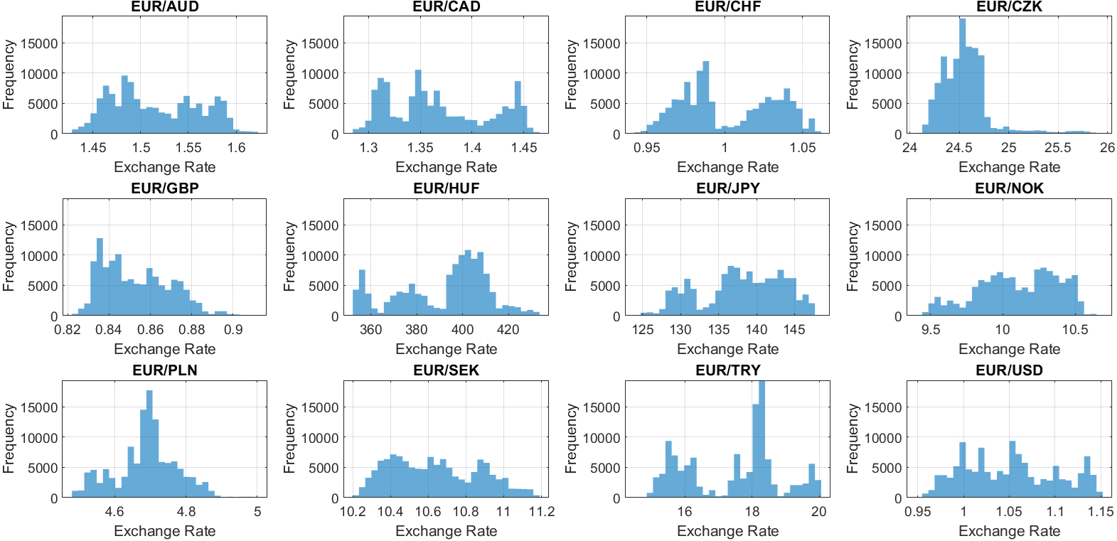
Boxplot of exchange rates.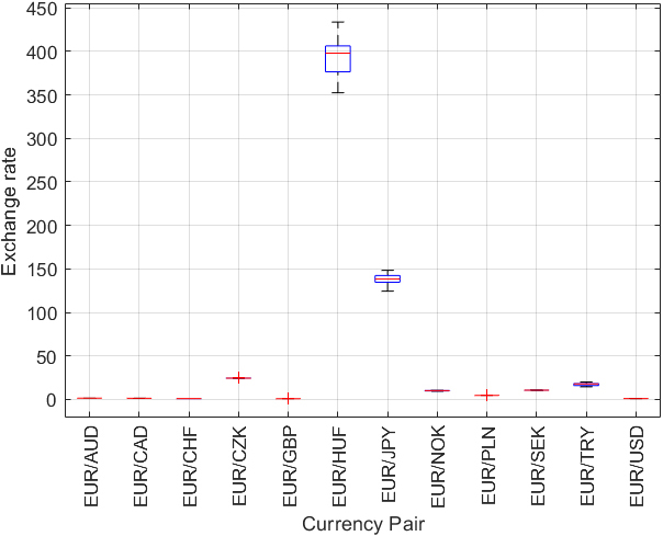
Exchange rates over time for EUR/PLN.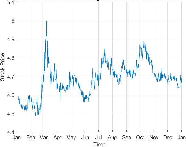
Rolling statistics of EUR/GBP.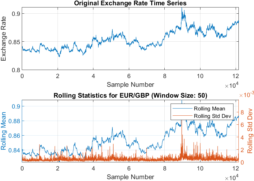
Rolling statistics of EUR/TRY.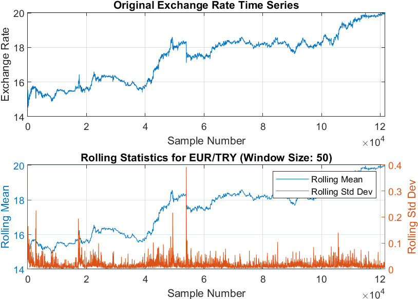
Correlation matrix of exchange rates.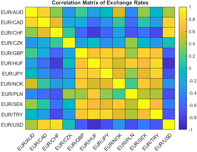
| DATE-TIME (EST) | EUR/AUD | EUR/CAD | EUR/CHF | EUR/CZK | EUR/GBP | EUR/HUF | EUR/JPY | EUR/NOK | EUR/PLN | EUR/SEK | EUR/TRY | EUR/USD |
|---|---|---|---|---|---|---|---|---|---|---|---|---|
| 2022-01-02 17:01 | 1.56356 | 1.43585 | 1.03628 | 24.8407 | 0.83937 | 369.317 | 130.743 | 10.00104 | 4.58643 | 10.26849 | 15.16616 | 1.1369 |
| 2022-01-02 17:02 | 1.56434 | 1.43547 | 1.03587 | 24.8444 | 0.83959 | 369.417 | 130.693 | 9.99679 | 4.58652 | 10.26961 | 15.16531 | 1.13689 |
| 2022-01-02 17:03 | 1.56446 | 1.43549 | 1.03652 | 24.8284 | 0.83954 | 369.512 | 130.707 | 10.00015 | 4.586 | 10.26588 | 15.21165 | 1.13692 |
| 2022-01-02 17:04 | 1.56474 | 1.43509 | 1.03626 | 24.8524 | 0.8391 | 369.538 | 130.756 | 9.99795 | 4.58624 | 10.27008 | 15.14329 | 1.13668 |
| 2022-01-02 17:05 | 1.56483 | 1.43575 | 1.03631 | 24.853 | 0.83974 | 369.538 | 130.765 | 9.99749 | 4.58575 | 10.27006 | 15.15891 | 1.13655 |
| 2022-01-02 17:06 | 1.56483 | 1.43547 | 1.0363 | 24.8608 | 0.83988 | 369.548 | 130.766 | 10.00545 | 4.58575 | 10.27175 | 15.1721 | 1.13682 |
| 2022-01-02 17:07 | 1.56482 | 1.43547 | 1.03587 | 24.8684 | 0.83992 | 369.553 | 130.755 | 10.00647 | 4.58623 | 10.27257 | 15.17382 | 1.13689 |
| 2022-01-02 17:08 | 1.56382 | 1.43594 | 1.03635 | 24.8694 | 0.83992 | 369.546 | 130.848 | 10.00594 | 4.58545 | 10.27388 | 15.20046 | 1.13682 |
| 2022-01-02 17:09 | 1.564 | 1.43547 | 1.03587 | 24.8623 | 0.8399 | 369.53 | 130.849 | 10.00599 | 4.58584 | 10.27481 | 15.22931 | 1.13723 |
| 2022-01-02 17:10 | 1.56425 | 1.43591 | 1.03587 | 24.8694 | 0.8399 | 369.516 | 130.848 | 10.00208 | 4.58486 | 10.27393 | 15.20626 | 1.13725 |
The mean, standard deviation, and interquartile range (IQR) of the exchange rates of each currency pair
The dataset encompasses 121,673 rows and 12 columns, representing minute-by-minute exchange rates for the specified currency pairs. The exploratory data analysis conducted on this dataset aimed to unveil its characteristics and dynamics. As a supplement to this description, the first few rows of the dataset are presented in Table 2. The Mean, Standard Deviation, and Interquartile Range (IQR) of the exchange rates of each currency pair are also given in Table 2. Five types of exploratory data analyses were performed, with the results visually represented in Figs 1 to 6.
Frequency Histograms of All Currency Pairs (Fig. 1): Frequency histograms of all currency pairs are shown in Fig. 1 to give a general overview of the dataset. Boxplots of Exchange Rates for all Currency Pairs (Fig. 2): Boxplots were created to provide an overview of each currency pair’s exchange rate distribution. They reveal essential statistical parameters such as the central tendency, spread, and potential outliers within each dataset. Exchange Rate Trend over Time (Fig. 3): A time-series plot for the exchange rate of EUR/PLN as a sample currency pair was drawn. This visualization helps identify the underlying patterns, trends, and fluctuations over the year. Rolling Statistics of Two Sample Currency Pairs (Figs 4 and 5): The rolling mean and the rolling standard deviation of the currency pairs EUR/GBP and EUR/TRY, as two sample exchange pairs, are presented in Figs 4 and 5, respectively. Correlation Matrix for all Currency Pairs’ Exchange Rates (Fig. 6): A correlation matrix was created to gain insights into the association degree and direction between different currency pairs’ exchange rates, illuminating positive, negative, or no correlation.
The aim of the data preprocessing stage was to optimize the data format for analysis and modeling. It consisted of two primary processes: missing data imputation and normalization.
Missing data points in the exchange rates were replaced by the average of the preceding and following minute’s exchanges rate for that currency pair, ensuring temporal continuity and minimizing potential bias or distortion.
Normalization, the next step, was carried out independently for each column in the dataset, corresponding to each currency pair, considering the different exchange rate magnitudes. The data was scaled into a [0,1] range, maintaining the original data pattern.
Lagged versions of the exchange rates for EUR/AUD, EUR/GBP, and EUR/PLN were created for supervised learning, representing the target values. The lagged time intervals included 1, 5, 10, 15, 30, 45, and 60 minutes. The stacked ensemble machine learning model was given 12 inputs for each minute, each representing a different currency pair’s current exchange rate, and a single target, which is the predicted future exchange rate for a specific currency pair. This approach encapsulated the interconnectedness of the currency exchange rates within the model.
Machine learning techniques and ensemble methods used
Support Vector Regression (SVR)
Support Vector Regression (SVR) is an innovative adaptation of the Support Vector Machine (SVM) algorithm, uniquely designed to accommodate regression tasks. SVR strives to devise a function that efficiently fits the training data whilst concurrently curbing the generalization error. This method stands out for its particular efficacy with high-dimensional datasets, and its resistance to overfitting surpasses several other regression methodologies.
SVR Formulation Consider a dataset encompassing The function
In this equation,
This is subject to the conditions: Here, Kernel Functions A kernel function SVR Algorithm Summary The generic procedure for constructing an SVR model for exchange rate prediction includes the following steps:
Select a kernel function and its parameters (for instance, RBF with a specified kernel scale). Define the margin of error Formulate and resolve the convex optimization problem to ascertain the optimal Lagrange multipliers Utilize the derived function
To conclude, SVR presents multiple benefits for predicting exchange rates. These encompass its capacity to depict non-linear relationships, resistance against overfitting, and appropriateness for high-dimensional datasets. Through judicious adjustment of the SVR model’s parameters, like the margin of error, kernel function, and box constraint, a harmonious equilibrium can be reached between the model’s precision and its complexity.
In this research, a grid search is executed to identify the optimal hyperparameters for the SVR model. The hyperparameters that were evaluated include:
Epsilon: This parameter sets a margin around the predicted values that disregard errors within its bounds. A broader margin and fewer support vectors result from a higher epsilon value, while a smaller epsilon results in a tighter margin and increased support vectors. Kernel scale: This scaling factor for the radial basis function (RBF) kernel governs the shape of the decision boundary. A more substantial kernel scale produces a smoother decision boundary, whereas a smaller kernel scale yields a more flexible boundary. Box constraint: This is a regularization parameter balancing minimizing training error and maximizing the margin. Larger values create a wider margin while tolerating some errors, whereas smaller values focus on minimizing training error.
A 5-fold cross-validation was used to identify the optimal hyperparameters. The training data was split into five equal portions, and in each iteration, four of these were used for training and one for testing. This procedure was conducted for all possible hyperparameter combinations.
For each hyperparameter set, the Mean Absolute Error (MAE) was computed for each fold, and then averaged across all folds to provide a single performance metric. The hyperparameter set resulting in the lowest average MAE was deemed the optimal one.
The optimal hyperparameters were found to be:
Epsilon: best_epsilon Kernel scale: best_kernel_scale Box constraint: best_box_constraint
The final SVR model was trained utilizing the complete training dataset and the optimal hyperparameters.
The Random Forest algorithm proceeds through the subsequent stages:
Create several bootstrapped samples from the training dataset. Construct a decision tree for each bootstrapped sample. While building each tree, a random subset of features is chosen for splitting at every node. Amalgamate the forecasts from all individual trees to create the final output.
The outcome of a Random Forest model for a specific input is mathematically represented as the average prediction from all individual decision trees:
where
where
Training the Random Forest Model In this research, a Random Forest model encompassing 50 decision trees is trained with the training dataset. The quantity of trees in the Random Forest is a vital hyperparameter impacting the model’s performance and generalization. Typically, a higher tree count enhances model accuracy but could increase computational expenses and the potential for overfitting. Predicting with the Random Forest Model Predictions with the trained Random Forest model are made by averaging the individual decision tree’s predictions for a given input, aiding in reducing prediction variance and enhancing model accuracy overall.
Conclusively, a Random Forest model with 50 decision trees was utilized to forecast changes in the future exchange rates of currency pairs based on the present minute’s exchange rates. By combining individual decision tree predictions, the Random Forest model offers a dependable and robust technique for predicting currency exchange rates.
In the current research, the number of trees in the random forest (num_trees) is initially established to 100. A random forest model is an aggregation of decision trees, and an increased number of trees usually enhances the model’s accuracy, but it might also incur higher computational expenses.
Subsequently, a grid search is executed to pinpoint the optimal hyperparameters for the random forest model. The hyperparameters scrutinized in this study included:
Minimum leaf size (min_leaf_size): This refers to the minimum count of observations in a leaf node. Lower values permit the trees to extend deeper, potentially leading to overfitting, whereas higher values could induce underfitting. Maximum number of splits (max_num_split): This sets the maximum number of divisions allowed in each tree, and consequently governs the complexity of the trees. Greater values facilitate more complex trees. Number of variables to sample (num_vars_to_sample): This determines the count of predictor variables chosen randomly at each division in the decision tree, thereby introducing variability in the tree building process, which can aid in enhancing generalization.
To discover the optimal hyperparameters, k-fold cross-validation is applied, with k set to 5. The training data was sectioned into five parts of equal size, with four segments being used for training and the remaining segment for testing during each iteration. This procedure was replicated for all potential hyperparameter combinations.
For each hyperparameter set, the Mean Absolute Error (MAE) was computed for each fold and averaged across all folds to yield a single performance metric. The hyperparameter set associated with the lowest average MAE was chosen as the optimal one.
The optimal hyperparameters discerned in this study were:
Minimum leaf size: optimal_min_leaf_size Maximum number of splits: optimal_max_num_split Number of variables to sample: optimal_num_vars
Finally, using the complete training dataset and the optimal hyperparameters, the final random forest model is trained.
On the designated dataset, the Support Vector Regression (SVR) method exhibits an average training time of 12,008 seconds, while the Random Forest method concludes training in an average of 1,763 seconds. These timings provide noteworthy insights into the computational requirements of each method. The evaluations were conducted on a high-performance computing system equipped with an 11
The discrepancy in training times between the Random Forest and SVR methods can be attributed to several factors. Notably, RF exhibits faster execution due to its algorithmic complexity, hyperparameter tuning requirements, parallelization capabilities, considerations of data size, and implementation optimizations.
Algorithmic Complexity: Random Forest involves building multiple decision trees during training, utilizing a parallelized process of recursively partitioning the data based on feature values. In contrast, SVR requires solving a mathematical optimization problem, which can be computationally intensive, particularly with large datasets. Hyperparameter Tuning: RF often requires fewer hyperparameters to tune, and default configurations may yield satisfactory results. Conversely, SVR involves tuning more hyperparameters, leading to an increased need for an exhaustive search over the hyperparameter space during training. Parallelization: RF benefits from parallelization, allowing the training of individual decision trees to occur concurrently. This parallel nature contributes to faster computation, especially on systems with multiple processors. SVR may face limitations in parallelization, potentially leading to longer training times. Data Size: RF efficiently handles large datasets, and its performance remains robust even with increasing data size. SVR, however, may experience longer training times as its computational complexity scales with the dataset size. Implementation and Optimization: The efficiency of RF is further enhanced by widely available, optimized implementations and integrated features like feature importance calculations. SVR, depending on the specific implementation and mathematical solver, may exhibit variations in efficiency.
In summary, the faster execution of the Random Forest method compared to SVR can be attributed to its algorithmic characteristics, ease of hyperparameter tuning, parallelization capabilities, robustness with larger datasets, and efficient implementation practices.
Average ensembling is an effective technique where the predictions from multiple models are combined by taking their average, which often leads to improved predictive performance. This is because averaging can help balance out the weaknesses of individual models and reduce variance. In this study, the average ensemble technique was applied to the predictions of the Support Vector Regression (SVR) and Random Forest models.
Mathematically, if there are
Stacking, also known as stacked generalization, is a methodology that uses an ensemble strategy. This involves training a secondary or meta-model to optimally integrate the predictions from multiple foundational models. The foundational models are trained using the original training data, and the meta-model is trained using the foundational models’ predictions on a distinct validation dataset. In this research, stacked ensembles are developed by leveraging decision tree, neural network, and random forest models as foundational models, with a variety of algorithms employed for the meta-model. The meta-model input is the validation data predictions from the foundational models. The composite prediction vector from all foundational models for a particular input
where
where
To provide a concise summary of the Stacked Ensemble of Random Forest and SVR method, the key snippets of the pseudocode that capture the essence of the algorithm are presented below. This abbreviated version is designed for readers seeking a quick reference to the fundamental steps and logic involved in the stacking process:
1. Convert response variable to double
2. Split data into training and testing sets
3. Set SVR hyperparameters and k-fold parameters
4. Initialize best mean absolute error for SVR
5. SVR Hyperparameter Tuning
a. Loop over epsilon, kernel_scale, box_constraint
i. Initialize error sum
ii. K-fold cross-validation for SVR
iii. Calculate average mean absolute error
iv. Update best hyperparameters if better
6. Train final SVR model with best hyperparameters
7. Make predictions on test data using SVR model
8. Set Random Forest hyperparameters and k-fold parameters
9. Initialize best mean absolute error for Random Forest
10. Random Forest Hyperparameter Tuning
a. Loop over min_leaf_size, max_num_split, num_vars
i. Initialize error sum
ii. K-fold cross-validation for Random Forest
iii. Calculate average mean absolute error
iv. Update best hyperparameters if better
11. Train final Random Forest model with best hyperparameters
12. Make predictions on test data using Random Forest model
13. Ensemble of SVR and Random Forest
14. Combine predictions into a matrix
15. Train linear regression model to combine predictions
16. Make predictions using stacked model
17. Calculate performance metrics
For a comprehensive understanding of the Stacked Ensemble of Random Forest and SVR method, the full pseudocode is included in the appendix. This detailed version outlines the algorithm’s step-by-step procedures, ensuring a thorough grasp of the intricacies involved in the stacking of Random Forest and Support Vector Regression models. Refer to the full pseudocode in the appendix for an in-depth exploration of the algorithm’s implementation.
In the present research, three assessment metrics were employed for evaluating the performance of both the individual and the ensemble models. The utilized metrics are the Mean Squared Error (MSE), the Mean Absolute Error (MAE), and the Mean Absolute Percentage Error (MAPE). The corresponding mathematical representations for these evaluation metrics are provided below:
where
Cross validation is a resampling technique used to evaluate machine learning models on a limited data sample. The goal is to assess how well the machine learning model is capable of predicting new data that was not used in model training.
One popular method is
ANOVA test
The Analysis of Variance (ANOVA) is a statistical method employed to ascertain the existence of significant differences between the means of two or more groups. In the context of ANOVA, the null hypothesis (H0) posits that the means of the groups under consideration are equal. If the derived p-value from the ANOVA test is lower than the predetermined significance level, typically 0.05, the null hypothesis is rejected. This rejection indicates the presence of a significant difference between the group means.
In the context of this research, the ANOVA test was implemented to compare the performance of the Support Vector Regression (SVR) and Random Forest (RF) models, which were the base models for the ensemble techniques. The application of the ANOVA test aimed to confirm a significant difference in the performance of these two models, hence justifying the utilization of an ensemble model combining these two distinct base models. By establishing a significant variance in their predictions, the rationale for ensembling these models to leverage their unique strengths and compensations, thereby improving the robustness and accuracy of predictions is provided.
The MSE, MAE, and MAPE values for the single RF, single SVR, average ensemble of RF
SVR, and stacked ensemble of RF
SVR models
The MSE, MAE, and MAPE values for the single RF, single SVR, average ensemble of RF
The results of the performance evaluation for single RF, single SVR, average ensemble of RF+SVR, and stacked ensemble of RF+SVR models on the test data are summarized in Table 3. It becomes readily apparent that the error metrics (Mean Squared Error, Mean Absolute Error, and Mean Absolute Percentage Error) are lowest for immediate (1-minute) predictions. As the forecast horizon lengthens, these error values naturally increase, reflecting the inherent difficulties in predicting long-term trends in the forex market. This progression highlights the necessity of frequently updating the prediction models with the most recent data. Such a dynamic approach enables the model to better navigate the volatility and unpredictable nature of currency exchange rate movements.
The 5-fold cross-validation results for the currency pairs EUR/AUD
The 5-fold cross-validation results for the currency pairs EUR/AUD
The 5-fold cross-validation results for the currency pairs EUR/GBP
Furthermore, a detailed presentation of the 5-fold cross-validation results for the currency pairs EUR/AUD, EUR/GBP, and EUR/PLN can be found in Tables 4, 5, and 6 respectively. These tables elucidate the robustness of the model across different data subsets, thus enhancing the confidence in its predictive capability.
The 5-fold cross-validation results for the currency pairs EUR/PLN
ANOVA test results of the RF and SVR base models
Additionally, the ANOVA test results, which provide statistical validation of the distinct performance of the RF and SVR base models, are encapsulated in Table 7. This rigorous statistical examination reinforces the decision to utilize these two distinct models within the stacked ensemble, enhancing both the robustness and generalizability of predictions.
The actual values vs. predicted output (left) and the scatter graph of the actual values vs. the predicted output of the next minute exchange rate by Stacked ensemble of Random Forest 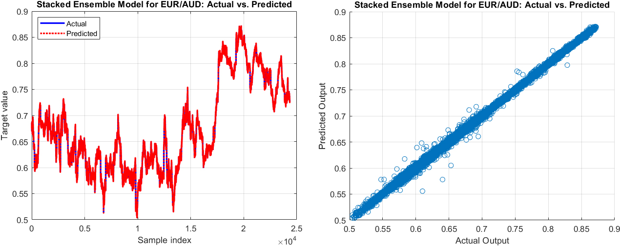
The actual values vs. predicted output (left) and the scatter graph of the actual values vs. the predicted output of the next 60-minute exchange rate by Stacked ensemble of Random Forest 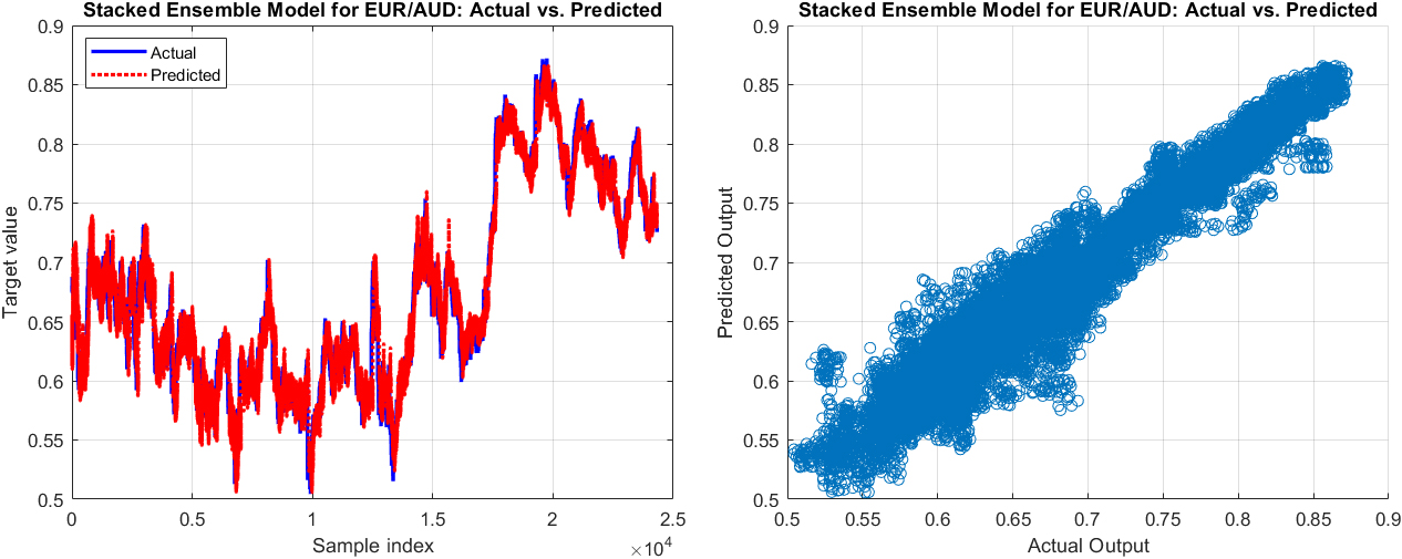
The actual values vs. predicted output (left) and the scatter graph of the actual values vs. the predicted output of the next minute exchange rate by Stacked ensemble of Random Forest 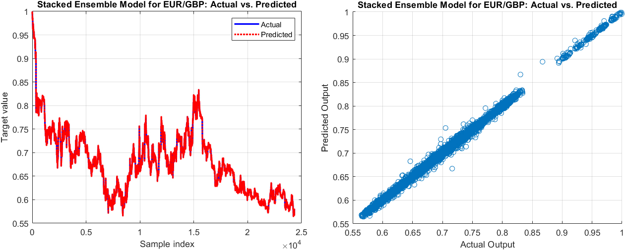
The actual values vs. predicted output (left) and the scatter graph of the actual values vs. the predicted output of the next 60-minute exchange rate by Stacked ensemble of Random Forest 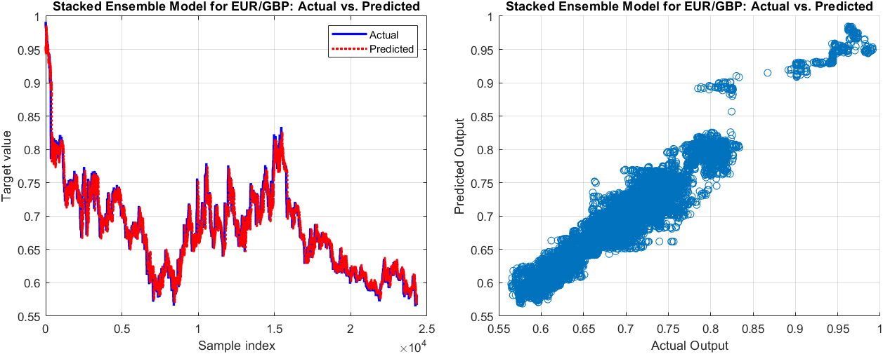
The actual values vs. predicted output (left) and the scatter graph of the actual values vs. the predicted output of the next minute exchange rate by Stacked ensemble of Random Forest 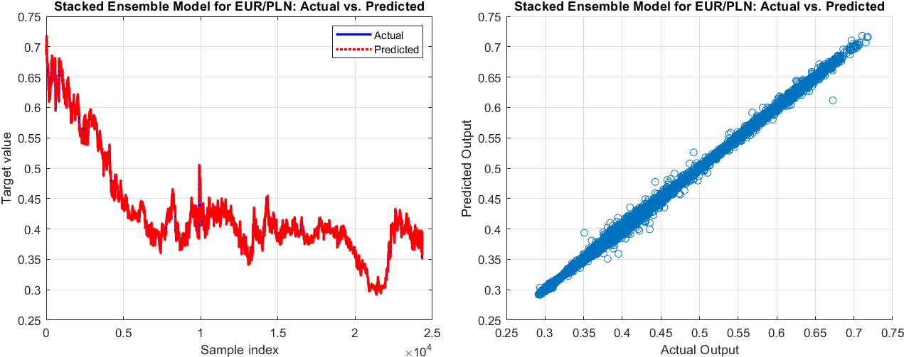
The actual values vs. predicted output (left) and the scatter graph of the actual values vs. the predicted output of the next 60-minute exchange rate by Stacked ensemble of Random Forest 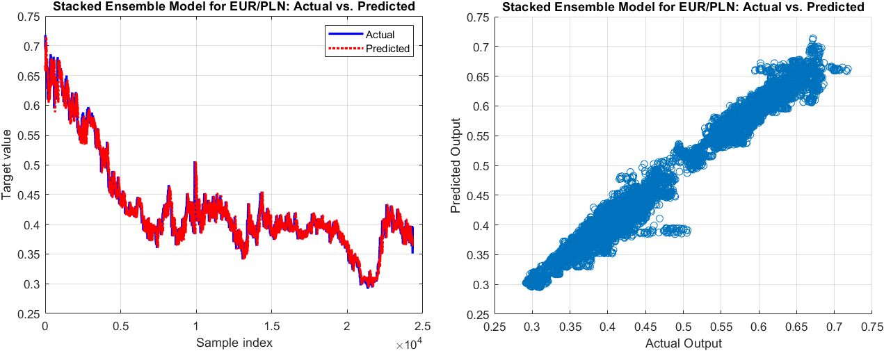
Figures 7–12 depict the comparison of actual versus predicted outputs, as well as scatter diagrams for the next 1 and 60 minutes of exchange rates for the currency pairs EUR/AUD, EUR/GBP, and EUR/PLN, respectively, using the stacked ensembles of Random Forest and SVR models. These visualizations are instrumental in comprehending the performance of the models in predicting immediate and longer-term future exchange rates. From a practical perspective, these models’ outputs, along with their accompanying visualizations, provide valuable insights for decision-making in foreign exchange (Forex) trading and risk management. Therefore, an in-depth analysis and discussion of these results are essential for a comprehensive understanding of the model’s performance and areas of potential improvement.
The examination of the performance metrics of the stacked ensemble model, which combines the Random Forest and SVR models, shows significant insights into its ability to predict the future exchange rates of various currency pairs.
Analyzing the Stacked Ensemble model’s performance across different currency pairs reveals some insightful patterns. For the EUR/AUD pair, the model showed a commendable precision with error metrics such as Mean Squared Error (MSE), Mean Absolute Error (MAE), and Mean Absolute Percentage Error (MAPE) being relatively low for short-term forecasts, particularly at the 1-minute mark. As anticipated, these error metrics progressively increased with longer prediction horizons, reflecting a natural growth in predictive uncertainty. Even at the 60-minute mark, the model maintained its efficacy with the MAPE just over 2%, indicating a commendable level of predictive accuracy, albeit the increment in forecast timeframe.
Turning to the EUR/GBP pair, the Stacked Ensemble model exhibited a superior performance. Despite the common trend of error rates escalating with longer prediction periods, the initial error rates for the EUR/GBP pair, as well as the growth rate of these errors, were notably lower compared to those observed in the EUR/AUD pair. Specifically, the 1-minute forecast started with a low MAPE of just above 0.16%, rising to slightly over 1.64% for the 60-minute prediction, which are the lowest figures among the three currency pairs evaluated. These results suggest a robust model performance when predicting the EUR/GBP exchange rate, potentially indicating a lower level of volatility or increased predictability for this currency pair compared to the others.
Lastly, for the EUR/PLN pair, the Stacked Ensemble model’s performance was somewhat similar to that of the EUR/AUD pair. However, even though the MAPE began just above 0.315% for the 1-minute forecast and slightly exceeded 2.31% for the 60-minute forecast, the model exhibited a high degree of accuracy, maintaining its predictive precision relatively well across all prediction intervals.
It’s important to bear in mind that these results do not necessarily reflect the model’s ability to capture all possible future scenarios. The real world of currency exchange rates is influenced by a myriad of factors including macroeconomic events, market sentiment, geopolitical developments and more. Nevertheless, the model’s ability to provide relatively accurate short-term predictions across multiple currency pairs is a positive indication of its usefulness as a tool in foreign exchange trading and risk management.
This study sets the groundwork for further exploration. While the proposed model shows promising results, additional research could be done to enhance its performance.
Conclusion
This study delves into the application of a stacked ensemble model, combining the strengths of Random Forest (RF) and Support Vector Regression (SVR), in predicting future exchange rates for several currency pairs. Performance evaluation was conducted using established measures such as Mean Squared Error (MSE), Mean Absolute Error (MAE), and Mean Absolute Percentage Error (MAPE). To offer a more holistic perspective, the model’s predictions were compared to those from individual RF and SVR models, as well as an averaged ensemble of the RF and SVR models.
To verify the reliability of the model, a k-fold cross-validation technique was used, with k set at 5. This method allowed a robust evaluation of the model’s predictive performance over different data subsets. Additionally, an Analysis of Variance (ANOVA) test was utilized, aimed at the RF and SVR base models. This test returned p-values in the range of 0.0103 to 0.0195, which strongly supports the distinctiveness of each base model in terms of performance. This validates the decision to construct a stacked ensemble model from two separate and unique base models, thereby increasing the robustness and generalizability of predictions.
The model was evaluated on three different currency pairs: EUR/AUD, EUR/GBP, and EUR/PLN. The findings confirmed the model’s ability to offer fairly accurate short-term predictions, though, as expected, the accuracy diminished as the prediction horizon increased. It was also observed that the model’s performance varied across different currency pairs, indicative of the unique characteristics and dynamics inherent to each pair.
In conclusion, the stacked ensemble model demonstrates significant promise as a valuable tool for predicting foreign exchange rates. Its performance, along with the additional layers of validation, including model comparisons, cross-validation, and ANOVA testing, underscores the potential of ensemble learning techniques. These techniques offer robust insights and enhance predictive performance in intricate, real-world contexts like financial markets.
Suggestions for future work
While the stacked ensemble model demonstrated promising results, there remains ample opportunity for further research and development to improve upon its performance and adaptability.
Model Diversity: Future research could explore incorporating a greater diversity of base models into the ensemble. Different machine learning algorithms excel in different aspects, and a more diverse ensemble might capture a broader spectrum of patterns in the data. Hyperparameter Tuning: Advanced techniques for hyperparameter tuning could potentially enhance the model performance. Approaches such as Bayesian optimization might be explored for more efficient and effective tuning processes. Feature Engineering: The features used in this study were relatively simple. More sophisticated feature engineering, such as inclusion of lagged variables or technical indicators, could potentially improve the model’s predictive power. External Factors: Incorporating external factors such as macroeconomic indicators or geopolitical events might improve the model’s ability to anticipate major shifts in exchange rates. Comparison with Other Ensemble Techniques: This study focused on stacking as the ensemble technique. Future work could compare the effectiveness of stacking with other ensemble methods like boosting or bagging in the context of exchange rate prediction. Deep Learning Models: Future research could also consider the application of deep learning models, which have shown strong performance in a variety of complex prediction tasks.
The state of the art in foreign exchange prediction can continue to advance by pursuing these and potentially other directions. This advancement aids practitioners in navigating this complex and critically important field.
Footnotes
Appendix
The full pseudocode of the Stacked Ensemble of Random Forest and SVR method:
1. // Convert the response variable to double
2. response = double(Total_out(:, 1));
3. // Split the data into training and testing sets
4. train_size = round(size(Total_in, 1) * 0.8);
5. train_in = Total_in(1:train_size, :);
6. train_out = response(1:train_size, :);
7. test_in = Total_in(train_size+1:end, :);
8. test_out = response(train_size+1:end, :);
9. // Set hyperparameters for SVR
10. epsilons = [0.01, 0.1, 1];
11. kernel_scales = [0.1, 1, 10];
12. box_constraints = [0.1, 1, 10, 100];
13. // Set k-fold cross-validation parameters for SVR
14. num_folds = 5;
15. cv = cvpartition(size(train_in, 1), ‘KFold’, num_folds);
16. // Initialize best mean absolute error for SVR
17. best_mae_svr = Inf;
18. // SVR Hyperparameter Tuning
19. for epsilon in epsilons:
20. for kernel_scale in kernel_scales:
21. for box_constraint in box_constraints:
22. mae_svr_temp_sum = 0;
23. // K-fold Cross-validation for SVR
24. for i in range(1, num_folds + 1):
25. train_in_fold = train_in(cv.training(i), :);
26. train_out_fold = train_out(cv.training(i));
27. test_in_fold = train_in(cv.test(i), :);
28. test_out_fold = train_out(cv.test(i));
29. // Train SVR model
30. svr_model_temp = fitrsvm(train_in_fold, train_out_fold, ‘Epsilon’, epsilon, ‘KernelScale’, kernel_scale, ‘BoxConstraint’, box_constraint);
31. // Predict using SVR model
32. svr_predictions_temp = predict(svr_model_temp, test_in_fold);
33. // Calculate mean absolute error
34. mae_svr_temp = mean(abs(test_out_fold - svr_predictions_temp));
35. mae_svr_temp_sum = mae_svr_temp_sum + mae_svr_temp;
36. end
37. // Calculate average mean absolute error for SVR
38. mae_svr_temp_avg = mae_svr_temp_sum / num_folds;
39. // Update best hyperparameters if current configuration is better
40. if mae_svr_temp_avg < best_mae_svr:
41. best_mae_svr = mae_svr_temp_avg;
42. best_hyperparams_svr = [epsilon, kernel_scale, box_constraint];
43. end
44. end
45. end
46. end
47. // Train the final SVR model with the best hyperparameters
48. best_epsilon = best_hyperparams_svr(1);
49. best_kernel_scale = best_hyperparams_svr(2);
50. best_box_constraint = best_hyperparams_svr(3);
51. svr_model = fitrsvm(train_in, train_out, ‘Epsilon’, best_epsilon, ‘KernelScale’, best_kernel_scale, ‘BoxConstraint’, best_box_constraint);
52. // Make predictions on the test data using the best SVR model
53. svr_predictions = predict(svr_model, test_in);
54. // Set hyperparameters for Random Forest
55. num_trees = 100;
56. min_leaf_sizes = [1, 5, 10, 20];
57. max_num_splits = [10, 20, 50, 100];
58. num_vars_to_sample = [5, 10, 20, 50];
59. // Set k-fold cross-validation parameters for Random Forest
60. num_folds = 5;
61. cv = cvpartition(size(train_in, 1), ‘KFold’, num_folds);
62. // Initialize best mean absolute error for Random Forest
63. best_mae = Inf;
64. // Random Forest Hyperparameter Tuning
65. for min_leaf_size in min_leaf_sizes:
66. for max_num_split in max_num_splits:
67. for num_vars in num_vars_to_sample:
68. mae_rf_temp_sum = 0;
69. // K-fold Cross-validation for Random Forest
70. for i in range(1, num_folds + 1):
71. train_in_fold = train_in(cv.training(i), :);
72. train_out_fold = train_out(cv.training(i));
73. test_in_fold = train_in(cv.test(i), :);
74. test_out_fold = train_out(cv.test(i));
75. // Train Random Forest model
76. Mdl_rf_temp = TreeBagger(num_trees, train_in_fold, train_out_fold, ‘Method’,
‘regression’, …
77. ‘MinLeafSize’, min_leaf_size, ‘MaxNumSplits’, max_num_split, …
78. ‘NumVariablesToSample’, num_vars);
79. // Predict using Random Forest model
80. predicted_out_rf_temp = predict(Mdl_rf_temp, test_in_fold);
81. // Calculate mean absolute error
82. mae_rf_temp = mean(abs(test_out_fold - predicted_out_rf_temp));
83. mae_rf_temp_sum = mae_rf_temp_sum + mae_rf_temp;
84. end
85. // Calculate average mean absolute error for Random Forest
86. mae_rf_temp_avg = mae_rf_temp_sum / num_folds;
87. // Update best hyperparameters if current configuration is better
88. if mae_rf_temp_avg < best_mae:
89. best_mae = mae_rf_temp_avg;
90. best_hyperparams = [min_leaf_size, max_num_split, num_vars];
91. end
92. end
93. end
94. end
95. // Train the final Random Forest model with the best hyperparameters
96. best_min_leaf_size = best_hyperparams(1);
97. best_max_num_split = best_hyperparams(2);
98. best_num_vars = best_hyperparams(3);
99. Mdl_rf = TreeBagger(num_trees, train_in, train_out, ‘Method’, ‘regression’, …
‘MinLeafSize’, best_min_leaf_size, ‘MaxNumSplits’, best_max_num_split, …
‘NumVariablesToSample’, best_num_vars);
100. // Make predictions on the test data using the best Random Forest model
101. predicted_out_rf = predict(Mdl_rf, test_in);
102. // Ensemble of SVR and Random Forest
103. // Combine the predictions
104. predicted_out_combined = [svr_predictions, predicted_out_rf];
105. // Bagging Ensemble
106. ens_bagging = fitensemble(predicted_out_combined, test_out, ‘Bag’, 200, ‘Tree’, ‘Type’, ‘Regression’);
107. predicted_out_bagging = predict(ens_bagging, predicted_out_combined);
108. // Boosting Ensemble
109. ens_boosting = fitensemble(predicted_out_combined, test_out, ‘LSBoost’, 200, ‘Tree’, ‘Type’, ‘Regression’);
110. predicted_out_boosting = predict(ens_boosting, predicted_out_combined);
111. // Weighted Average Ensemble
112. wa_ens = (svr_predictions * 0.5) + (predicted_out_rf * 0.5);
113. // Combine the predictions into a matrix
114. predicted_out_combined = [svr_predictions, predicted_out_rf, predicted_out_bagging, predicted_out_boosting];
115. // Train a linear regression model to combine the predictions
116. stacked_model = fitlm(predicted_out_combined, test_out);
117. predicted_out_stacked = predict(stacked_model, predicted_out_combined);
118. // Calculate performance metrics