Sage Journals: Discover world-class research

Abstract

Temporal link prediction based on graph neural networks has become a hot spot in the field of complex networks. To solve the problems of the existing temporal link prediction methods based on graph neural networks do not consider the future time-domain features and spatial-domain features are limited used, this paper proposes a novel temporal link prediction method based on two streams adaptive graph neural networks. Firstly, the network topology features are extracted from the micro, meso, and middle perspectives. Combined with the adaptive mechanism of convolution and self-attention, the preprocessing of the feature extraction is more effective; Secondly, an extended bi-directional long short-term memory network is proposed, which uses graph convolution to process topological features, and recursively learns the state vectors of the target snapshot by using the future time-domain information and the past historical information; Thirdly, the location coding is replaced by the time-coding for the transformer mechanism, so that past information and future information can be learned from each other, and the time-domain information of the network can be further mined; Finally, a novel two-stream network framework is proposed, which combines the processing results of point features and edge features. The experimental results on 9 data sets show that the proposed method has a better prediction effect and better robustness than the classical graph neural network methods.

Keywords

Temporal link prediction adaptive features fusion multi-convolution extended BiLSTM two stream network

1. Introduction

The networks in the real world are changing dynamically with time. The topology of the dynamic network is evolving and updating [1], where a new edge appears and the old disappears. Real-world networks and various graph signals could be regarded as dynamic networks. Graph signal processing often uses spectral estimation, probability reasoning, statistical learning, etc. [2] Link prediction based on a graph neural network model is an essential branch of graph signal analysis used to predict the future or reconstruct the network topology.

Many existing temporal link prediction methods based on the traditional static link prediction indices, regarded static snapshots as an unweighted training graph or a weighted cumulative graph for similarity training [3]; Many scholars have studied the methods which combine static similarity indices with time series analysis models. After calculating the static indices of each snapshot, combined with moving average, regression, and exponential smoothing, the results can express the prediction of network topology [4]; Drawing on the strong ability of representation learning for feature information extraction, the researchers have proposed DeepWalk [5], node2vec [6], LINE (Large scale Information Network Embedding) [7] based on node random walk and shallow neural network, which can also effectively realize temporal link prediction.

With the graph neural network to mine more effective spatial and temporal features, this paper proposes a novel temporal link prediction method based on two streams adaptive graph neural network, which can effectively learn the spatial and time information of the dynamic network. The model designs adaptive preprocessing of multi-dimensional topological features and proposes an encoding layer based on the extended bidirectional LSTM model and the optimized transformer model, as well as the two stream processing architecture for node feature data stream and edge feature data stream. The highlights are listed as follows:

(1)
For the precoding process, combined with convolution and self-attention mechanism, an adaptive feature processing method is proposed to extract network structure features from the micro, meso, and middle perspectives. A novel multi-layer GCN and GAT is proposed to mine more information on the network.
(2)
For the training and learning process, a novel BiLSTM model is proposed, which uses GCN to process spatial-domain information. It also combines the future and past time-domain data to predict the network. And a novel time coding mechanism is proposed to replace the position-coding for the transformer encoder.
(3)
For the decoding process, a novel two-stream network model is proposed. The results of node and edge features are fused to form the final representation vector. And the multi-layer perception is used to achieve temporal link prediction.
(4)
The experimental results on 9 data sets show that compared with several classical methods based on the GNN model, the proposed method achieves better prediction performance.

2. Related work

To mine effectively the evolution information of dynamic networks, dynamic graph neural network (DGNN) models are increasingly used in the field of complex networks. When dynamic networks are processed by discrete snapshots, they can be modeled in three ways: stacking DGNN, integrated DGNN, and dynamic graph automatic encoder [8].

Stacked DGNN-based models use static graph models to process each snapshot, which can get the node feature representations through end-to-end learning. GNN can capture the nonlinear relationship between nodes, and combine recurrent neural network (RNN) models to process the time-domain information of network evolution [9], which can more effectively aggregate node embedded representations at different moments, and significantly improve the accuracy of temporal link prediction. Liu et al. proposed a new graph convolution network (GCN) model, which uses GCN to process node features and k-core method decomposition features, and then uses a recurrent neural network to process the representation vector at each time [10]. Manessi et al. proposed WD-GCN (Waterfall Dynamic GCN) and CD-GCN (Concatenated Dynamic GCN). These two models also use GCN to process each snapshot and use LSTM models for each node [11]. Many other scholars have used the graph attention networks model to replace the standardized operations in GCN [12]. GAT can use the self-attention layer to learn the different effects of the neighbor node on the central node and give them different weights to focus on the key features. Zhang et al. proposed the Gated Graph Attention Network, the performance was further improved by combining gating and attention mechanisms [13]. Sankar et al. proposed the DySAT model by combining GAT with the temporal self-attention mechanism. This model first uses GAT to process the spatial structure features of each snapshot, and it uses the self-attention mechanism to extract the time-domain features contained in the network snapshots to obtain the representation vector of historical information [14].

The model based on integrated DGNN integrates GNNs with RNNs, instead of separately processing according to spatial-domain and time-domain. GConvLSTM model uses both temporal and spatial information to change the connection weight in LSTM to convolution operation [15]. EvolveGCN also integrated GNN and RNN, and the model updated the GNN coefficient matrix using the RNN method [16]. Wang et al. proposed the ST-LSTM model, which processes spatial and temporal information in a memory processing unit and transfers memory messages in horizontal and vertical directions. Input parameters are not only the hidden state but also cell state with the previous time step from the two directions[17]. GC-LSTM model regards LSTM as a hidden layer and uses GCN to process the input and output of the hidden layer. It takes the adjacency matrix as the input parameter to LSTM, and proposes a new graph convolution model in the hidden layer [18]. Similarly, the LRGCN model integrates the improved R-GCN [19] with LSTM in the hidden layer, which can realize the state embedding analysis in the dynamic network [20]. ReNet model integrates stacked R-GCNs into a dynamic knowledge map for complex network analysis [21]. Bonner et al. designed a two-layer Temporary Neighbourhood Aggregation (TNA) model uses hierarchical convolution with different depths and adjustable variational sampling [22].

The model based on GAE (Graph Auto Encoder) regards DGNN as an encoder. Reference [23] proposed the DyLink2Vec model, which uses an optimization coding mechanism to improve representation learning. DyLink2Vec consists of two steps: compression and reconstruction. The goal is to minimize reconstruction error and use the gradient descent method to optimize the training process. DynGEM model optimizes the self-encoder by using the weight of the snapshot at the previous time based on static graph self-coding [24]. The E-LSTM-D model has designed the encoding layer, stacked LSTM blocks, and decoding layer. At the encoding layer, LSTM is used to handle the representation vector of nodes. The encoder realizes the learning of complex network structures. The stacked LSTM blocks learn the time evolution features. The decoder converts the extracted features to the original space for prediction [25]. The GraphSAGE model proposed by Hamilton et al. optimizes the encoder. First, it uses uniform sampling to fix neighborhood nodes and uses different aggregation functions to handle neighborhood information aggregation [26]. Hajiramezanali et al. introduced the variational mechanism and proposed two kinds of variational self-encoders for dynamic networks, including the Variational Graph Recurrent Neural Network (VGRNN) and Semi implicit VGRNN (SI-VGRNN). These two models both integrate GCN into RNN as an encoder, which could get more optimized node representation vectors [27]. LI et al. proposed the TSAM model, which uses the graph attention network to process the structural features, and uses the gated loop unit to extract the temporal evolution features from the network snapshots. And the model also uses the self-attention mechanism to focus on the more important network snapshots [28].

Summarize the above three kinds of models based on the graph neural network. On the one hand, GNN-based models include GCN, GAT, GAE, and RNN-based models include LSTM, GRU, etc. The optimization efforts of these models do not focus on further research on the design of input and output. On the other hand, when using RNN to process the time evolution information, the prediction function often uses past historical information to predict the network topology but does not use future information.

3. Preliminary

3.1 Problem definition

It is common to divide the dynamic network into a series of snapshots with the same interval. Then we can research various complex network tasks based on the discrete graphs. The discrete DGNN method can not only use the time series analysis models to handle the evolution information but also easily use the graph neural network model for learning structure information. Given a discrete dynamic network, it can be divided into some snapshots at a fixed time interval, and the general model for graph neural network training is shown in Eq. (1):

$\displaystyle z_{1}^{t},z_{2}^{t},\ldots,z_{n}^{t}=\textit{GNN}({G^{t}})$ (1) $\displaystyle h_{j}^{t}=\textit{RNN}(h_{j}^{t-1},z_{j}^{t})\ \textit{for}\ j% \in[1,n]$

where $n$ is the number of nodes, $z_{i}^{t}$ is the output state representation vector of node $i$ at time $t$ , GNN is the graph neural network model, usually including GCN, GAT, and other models based on spectral or spatial domain, $h_{j}^{t}$ is the memory state representation vector of node $j$ at time $t$ , and RNN is the recurrent neural network model, usually including GRU, LSTM and other models. Equation (1) can also be expressed as:

$\displaystyle{{\bf{Z}}^{t}}=\textit{GNN}({G^{t}})$ (2) $\displaystyle{{\bf{H}}^{t}}=\textit{RNN}({{\bf{H}}^{t-1}},{{\bf{Z}}^{t}})$

where ${\bf{Z}}^{t}$ can be regarded as the output results of the spatial-domain structure feature at time $t$ , and ${{\bf{H}}^{t}}$ can be regarded as the output results of the time-domain evolution feature between time $t$ and time $t-1$ .

The temporal link prediction problem based on a neural network model can be summarized into the following three steps:

(1)

Aiming at the spatial features of the dynamic network structure information, the GNN optimization models are studied;

(2)

Aiming at the time features of the dynamic network evolution information, the RNN optimization models are studied;

(3)

According to the final output representation vectors, the prediction and evaluation of the network topology can be realized.

3.2 Metrics

The evaluation Metrics commonly used to measure the performance of link prediction methods, mainly including AUC (Area Under Curve), Brier Score, MAP (Mean Average Precision), MAE (Mean Absolute Error), RMSE (Root Mean Square Error), etc. [29].

The AUC metric is widely used to measure the accuracy of prediction methods. The measurement of this index is in the range of [0,1]. For $n$ times independent comparison, $n^{\prime}$ if the scores of random edges are greater than those of nonexistent edges, and $n^{\prime\prime}$ if the scores are equal, then AUC can be expressed as:

$\displaystyle\text{AUC}=\frac{{n^{\prime}+0.5n^{\prime\prime}}}{n}$ (3)

The Brier metric can be considered as a measure of the calibration of a set of probability predictions. The corresponding cases of this set of probabilities must be mutually exclusive, and the sum of probabilities must be 1. The lower the Brier score for a set of predicted values, the better the prediction calibration. The Brier Score can be expressed as:

$\displaystyle\text{Brier}=\frac{1}{n}\sum\limits_{i=1}^{n}{{{({y_{i}}-\hat{y_{% i}})}^{2}}}$ (4)

The MAP metric is the mean average precision value, representing the geometric average value of the accuracy of all categories. The link prediction problem is essentially a binary classification problem. Precision reflects the proportion of the samples predicted to be Class $i$ . As shown in Eq. (5). First, calculate the precision scores of n categories, and get the average precision AP score of each category. Then, calculate the geometric mean according to the classification. The link prediction belongs to the binary classification, it can set $m=2$ .

$\displaystyle\textit{AP}=\frac{1}{n}\sum{\textit{Precision(i)}}$ (5) $\displaystyle\textit{MAP}=\frac{1}{m}\sum{\textit{AP}}$

The MAE index is the mean absolute error value, which represents the average of the absolute value of the error between the predicted and the real value, which can better reflect the actual performance of the methods. The RMSE index is the root mean square error value, which can measure the deviation between the two values and be sensitive to abnormal data. As shown in Eq. (3.2), $m$ is the number of snapshots of the test set graph, $y_{i}$ is the label value, and $\hat{y_{i}}$ is the predicted probability value.

$\displaystyle\textit{MAE}=\frac{1}{m}\sum\limits_{i=1}^{m}{\left|{({y_{i}}-{y_% {i}})}\right|}$ (6) $\displaystyle\textit{RMSE}=\sqrt{\frac{1}{m}\sum\limits_{i=1}^{m}{{{({y_{i}}-% \hat{y_{i}})}^{2}}}}$

4. Method

The existing graph neural network methods do not consider the diverse scenarios of input feature parameters, and they mine the future time-domain features and spatial-domain features limited. A novel temporal link prediction method based on two streams adaptive graph neural network (TSAGNN) is proposed, which can fully learn the spatial and temporal information of the dynamic network. As shown in Fig. 1, the TSAGNN consists of the AGBLTE model and decoder model, including the adaptive graph convolution attention layer (AGA), the extended long short-term memory network layer (exBiLSTM), the transformer encoder layer and the decoder layer.

Figure 1.

Overall logic architecture of TSAGNN.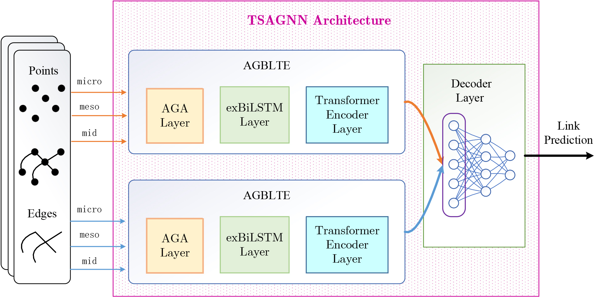

First, the AGA layer proposes a novel adaptive mechanism, which combines some GNN and GAT layers for the spatiotemporal features from different scales of network structures. After convolution and self-attention processing for the input, the features of different scales are transformed into the same dimension and adaptively perform depth coupling on each other according to the feature weight. Secondly, the exBiLSTM layer further mines spatial features by using GCN to process topology information between LSTM cells, while the exBiLSTM layer makes full use of the time-domain characteristics of the network at the same time. Based on the LSTM network, it supports the simultaneous learning of the past and future network data. After processing the past and future information respectively, it fuses the past and future results as the state information of the target time. Thirdly, the Transformer Encoder layer further optimizes the output vector results and proposes a new time-encoding to replace the position-encoding for the encoder, while using the Transformer’s mechanism to realize mutual learning between past and future information. Finally, the decoder layer is proposed based on the two-stream network architecture, which consists of multi-layer perception (MLP). The processing results of node features and edge features are handled respectively. The full connection network is used to process the feature vector of two stream outputs, which makes sense to the temporal link prediction method based on TSAGNN.

4.1 Adaptive graph convolution attention layer

The input parameters of GNN models such as GCN or GAT include adjacency matrix and eigenvectors of all nodes. The eigenvectors of nodes can be label attributes, similarity indices, walking representation vectors, etc. The general GNN model uses the label attribute or one hot vector to represent the feature of the node. A novel adaptive convolution processing layer is designed, as shown in Fig. 2. Specific details of the AGA layer are as follows: a set of mapping functions is defined to extract the features of the input adjacency matrix, and the topological similarity of different perspectives is considered. After multiple convolutions and self-attention operations, we set adjustment parameters to make features fusion adaptively according to the different weights.

Figure 2.

Schematic diagram of adaptive convolution processing layer.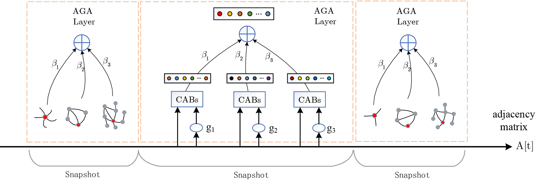

4.1.1 Input Multi-perspective node features

The structure of complex networks can be classified from different perspectives, such as the microscopic, mesoscopic, and midscopic. The stability, density, and concentration of nodes can represent the micro features of nodes. The characteristics of motifs can represent the mesoscopic features of the local network structure. The random walking vector and community centrality within subgraphs can represent the midscopic features of networks. At last, an adaptive adjustment mechanism is used in the final feature fusion according to the score proportion of these different features.

From a microscopic perspective, based on the sociological influence, the more neighbors a user has, the greater its influence is. The micro similarity of nodes can be characterized by the first-order and second-order degrees of nodes [30], as shown in Eq. (7), $\lambda$ is the second-order adjustment coefficient, $j$ is the neighbor set of node $i$ and is the degree of node $i$ .

$\displaystyle{g_{1}}(i)={k_{i}}+\lambda\cdot\sum\limits_{j\in\Gamma(i)}{{k_{j}}}$ (7)

From a mesoscopic perspective, the number of the most basic triangular motifs of the network also can be used to represent the influence of a node. The larger the number of motifs, the greater its influence is. The mesoscopic similarity can be characterized by the first-order and second-order number of triangular motifs, as shown in Eq. (8), $\lambda$ is the second-order adjustment coefficient, $M_{i}$ is the number of triangular motifs of node $i$ , and $j$ is the neighbor set of node $i$ .

$\displaystyle{g_{2}}(i)={M_{i}}+\lambda\cdot\sum\limits_{j\in\Gamma(i)}{{M_{j}}}$ (8)

From a midscopic perspective, the centrality of the subgraph eigenvector can be used to represent the influence of nodes. First, the network is divided into some communities. Then, the first-order and second-order centrality indices of nodes within the community are used to represent the midscopic similarity, as shown in Eq. (9), $\lambda^{\prime}$ is a constant parameter, cen is the node centrality function, and node $i$ and node $j$ both belong to the same community.

$\displaystyle{g_{3}}(i)={\lambda}^{{}^{\prime}}\cdot\sum\limits_{j\in\Gamma(i)% }A(i,j)\cdot\textit{cen}(j)|\ i,j\in{C_{k}}$ (9)

The feature mapping functions are not limited to the above three types. From the micro perspective, the reciprocal of degree, the label attributes of nodes, or other local structure similarity indices can also be used to characterize nodes; From the mesoscopic perspective, except using triangular motifs, the common features of quaternion motifs can also be taken into account; From the midscopic perspective, the similarity can also use the path feature, as well as other centrality indices such as betweenness centrality and closeness centrality, etc.

4.1.2 Multi-convolution attention layer and feature aggregation

The feature dimensions after mapping and processing from different perspectives are different. The graph neural network is used to further mine the network’s spatial information, and multiple convolution attention blocks (CABs) are designed to process the input features. After two convolution layers and two self-attention layers, the feature dimensions of all outputs are the same dimensions. Then, we put the node features and adjacent matrix into CABs to realize convolution and attention processing, as shown in Fig. 3.

Figure 3.

Schematic diagram of feature fusion processing module.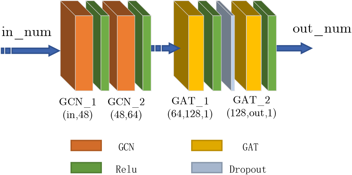

By capturing the adjacent information propagation process in the graph topology, the specific implementation of the GCN processing unit can be expressed as Eq. (10).

$\displaystyle{H^{(l+1)}}=\sigma({\tilde{D}^{-\frac{1}{2}}}\tilde{A}{\tilde{D}^% {-\frac{1}{2}}}{H^{(l)}}{W^{(l)}})$ (10)

where $\tilde{A}=A+I$ is the sum of the adjacent matrix and identity matrix, which brings the node self-connection feature in the training process. $\tilde{D}=\sum{{{\tilde{A}}_{ij}}}$ is a degree matrix, ${H^{(l)}}$ is the output state of layer l and ${W^{(l)}}$ is the training parameter of layer $l$ . Based on one-layer processing, this paper designs a two-layer GCN convolution operation, as shown in Eq. (11), to obtain the state vector of each node at the current time.

$\displaystyle\textit{GCN}(A,X)=\sigma(\mathord{\buildrel{\lower 3.0pt\hbox{$% \scriptscriptstyle\frown$}}\over{A}}\cdot Relu(\mathord{\buildrel{\lower 3.0pt% \hbox{$\scriptscriptstyle\frown$}}\over{A}}X{W_{0}}){W_{1}})$ (11)

where X is the input node feature matrix, A is the adjacent matrix, and $\sigma(\cdot)$ and $\textit{Relu}(\cdot)$ are the nonlinear activation function, $\mathord{\buildrel{\lower 3.0pt\hbox{$\scriptscriptstyle\frown$}}\over{A}}={% \tilde{D}^{-\frac{1}{2}}}\tilde{A}{\tilde{D}^{-\frac{1}{2}}}$ is the normalized matrix parameter in the training process, ${W_{0}}$ and ${W_{1}}$ are the training weight parameters of the first and second layers.

After the two-layer convolution operation, combined with the influence of the neighbor information, the attention mechanism is used to optimize the output state vector. $h(i=\textit{GCN}(A,{X_{i}})$ is the output state vector of node $i$ , the two-layer attention processing function is also defined, as shown in Eq. (12).

$\displaystyle{e_{i}}={w_{2}}({w_{1}}H+{b_{1}})+{b_{2}}$ (12)

where $H$ is the output result of Eq. (11), $w_{1}$ and $b_{1}$ are the first layer attention weight parameter and offset, $w_{2}$ and $b_{2}$ are the second layer attention weight parameter and offset.

The attention coefficient ${e_{ij}}$ represents the influence of node $j$ on node $i$ . Masked attention is used to softmax normalize the attention coefficient with the node’s first-order neighbor, as shown in Eq. (13).

$\displaystyle{\alpha_{i}}=\frac{{\textit{exp}({e_{i}})}}{{\sum\nolimits_{j=1}^% {n}{\exp({e_{j}})}}}$ (13)

Then, the attention coefficient of the neighbor node set is weighted and summed to obtain the final output parameters, as shown in Eq. (14).

$\displaystyle C(i)=\sum\limits_{j=1}^{n}{{\alpha_{j}}\cdot{h_{j}}}$ (14)

Finally, the features of nodes are quantized from multiple perspectives, and the results processed by CABs are adaptively fused. The output results are normalized, and the fusion factor is defined to represent the weight proportion of each feature. The calculation is shown in Eq. (15). The vector inner product method is used to fuse multiple output state vectors, such as Eq. (16), where $k$ is the type of the mapping function, and Normize is the normalized processing function, $X$ is the feature vector after adaptive fusion.

$\displaystyle{\beta_{k}}(i)=\left.\frac{{\textit{Normlize}({g_{k}}(i))}}{{\sum% {\textit{Normlize}({g_{k}}(i))}}}\right|\ k=1,2,3\ldots$ (15) $\displaystyle X(i)=\sum{{C_{k}}(i)\cdot{\beta_{k}}}(i)$ (16)

4.2 Extended bidirectional long short-term network layer

RNN is generally used to process time series data or semantic data, but the output of each layer of RNN can only affect adjacent moments and does not support long-term impact. GRU and LSTM both can solve this problem. Based on LSTM, this paper designs an extended bidirectional LSTM mechanism and reconstructs the present network topology by combining the past and future time domain information.

Most prediction tasks are based on past historical information to achieve the prediction. The output at the current time is not only related to the historical state of the time series data but also related to the future topology state. For example, to predict the missing words in a sentence, you need to not only handle the preceding text but also consider the content behind it so that you can judge based on the context.

Figure 4.

Schematic diagram of extended bidirectional long short-term memory network.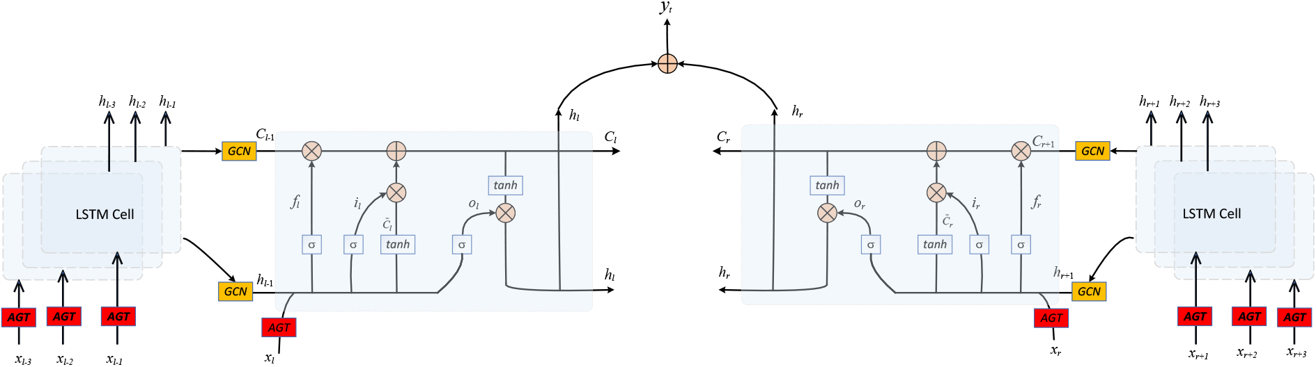

Three gate structures are designed in LSTM, which are the forgetting gate, input gate, and output gate. They are used to realize information forgetting, long-term memory, and short-term memory. Usually, bidirectional LSTM performs forward and reverse two-loop processing on time series data, and concatenates the final results. In this paper, an extended bidirectional long short-term memory network is proposed. As shown in Fig. 4, the past time snapshots are represented by variable $l$ , variable $p$ represents the size of the bidirectional moving window, and the time series data is recursively calculated from $l-p$ to $l$ . At the same time, the future time snapshots are represented by variable $r$ , and the time series data is recursively calculated from $r+p$ to $r$ . LSTM is performed both from the past and the future simultaneously, and the output vectors from both sides are concatenated. In addition, the long-term and short-term memory states information of each LSTM cell designed in this paper needs to be handled by GCN. After the further process of the spatial features evolved by time series, they are transmitted to the next LSTM cell. The specific implementation steps are as follows:

Firstly, according to the step size $p$ of the training window, the corresponding time series data set is split as left and right training sets for each target time, $x$ is the original feature of the network topology, and $X$ is the output feature vector processed by the AGA layer.

Secondly, the data at each moment is input into the LSTM cell for training. The GCN is used to process the short-term state $h$ and long-term state $C$ , and learn from the new input feature $X$ , such as Eqs (17)–(19) to update the forgetting gate, input gate, and cell state.

$\displaystyle{f_{t}}=\sigma({W_{f}}\cdot\textit{GCN}({h_{t-1}},{X_{t}})+{b_{f}})$ (17) $\displaystyle{i_{t}}=\sigma({W_{i}}\cdot\textit{GCN}({h_{t-1}},{X_{t}})+{b_{i}})$ (18) $\displaystyle{\tilde{C}_{t}}=\textit{tanh}({W_{c}}\cdot\textit{GCN}({h_{t-1}},% {X_{t}})+{b_{c}})$ (19)

Thirdly, calculate and output the long-term state and short-term state of the LSTM cell, as shown in Eqs (20)–(22).

$\displaystyle{C_{t}}={f_{t}}*{C_{t-1}}+{i_{t}}*{\tilde{C}_{t}}$ (20) $\displaystyle{O_{t}}=\sigma({W_{o}}\cdot\textit{GCN}({h_{t-1}},{X_{t}})+{b_{o}})$ (21) $\displaystyle{h_{t}}={O_{t}}*\textit{tanh}({C_{t}})$ (22)

Finally, the left series and right series are trained respectively, and the final hidden state vector $h$ is concatenated from both sides to obtain the state representation vector at the target time $t$ . In Eq. (23), mul represents coupling processing function.

$\displaystyle{y_{t}}=\textit{mul}({h_{l}},{h_{r}})$ (23)

The ExBiLSTM layer uses the Adam optimizer to optimize the model. The loss function of the training process is defined in Eq. (24), which represents the error between the prediction expectation and the true labels.

$\displaystyle\textit{loss}=\frac{1}{m}\sum\limits_{i=1}^{m}{{{({Y_{t}}-{{% \mathord{\buildrel{\lower 3.0pt\hbox{$\scriptscriptstyle\frown$}}\over{Y}}}_{t% }})}^{2}}}$ (24)

4.3 Transformer encode layer based on time-coding

Based on the attention mechanism, Google also proposed Transformer [31] model by using the stacked Encoder Decoder structure. It completely uses the attention method to replace the RNN serialization function. Through the training of different weight matrices, it can achieve better results by the attention mechanism. Because the model discards the time attribute of the sequence, it designs a position-coding mechanism, which endows each node with corresponding position information.

Figure 5.

Functional Diagram of Transformer Coding Layer. (a) Transformer Encoder. (b) Multiple attention mechanism.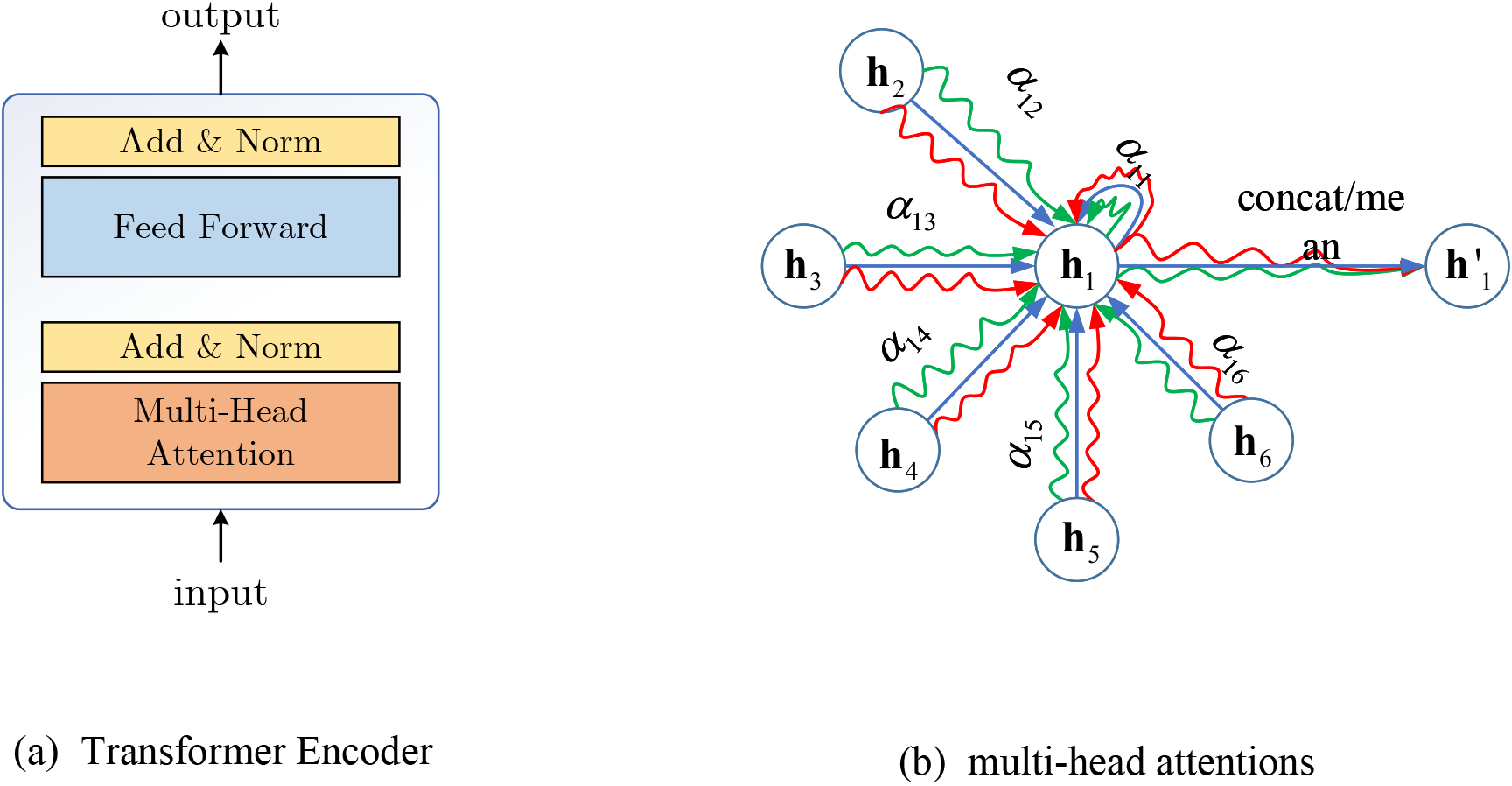

Although the exBiLSTM model uses the history and future data for training, the time evolution information of their sequences is learned respectively. However, future information has an impact on the current time and the past time. Similarly, historical information has an impact on the future. For further utilization of the network time-domain information, two sequences can learn from each other. Based on the mechanism of the Transformer coding layer to handle the node state vector information, we can further mine the context information of the network data by replacing the position-coding with the timing coding. As shown in Fig. 5(a), the Transformer coding layer includes the multi-head attention mechanism, the Add&Norm layer, and the Feed Forward layer. As shown in Fig. 5(b), the multi-attention mechanism is used to get more semantic information and concatenate or average the results to get the final value. After the weighted sum of attention is updated by the activation functions, the feature vector of the node can be expressed as Eq. (25). When considering that the sum of the weights of all neighbors is 1, use multiple heads of attention for processing, and the calculation can be shown in Eqs (26)–(27).

$\displaystyle\bf{h^{\prime}}_{i}=\sigma\left(\sum\limits_{j\in\Gamma\left({{v_% {i}}}\right)}\alpha_{ij}{\bf{Wh}}_{j}\right)$ (25) $\displaystyle{\bf{h}}_{i}^{\prime}=||_{k=1}^{K}\sigma\left({\sum\limits_{j\in% \Gamma\left({{v_{i}}}\right)}{\alpha_{ij}^{k}{{\bf{W}}^{k}}{{\bf{h}}_{j}}}}\right)$ (26) $\displaystyle{\bf{h}}_{i}^{\prime}=\sigma\left({\frac{1}{K}\sum\limits_{k=1}^{% K}{\sum\limits_{j\in\Gamma\left({{v_{i}}}\right)}{\alpha_{ij}^{k}{{\bf{W}}^{k}% }{{\bf{h}}_{j}}}}}\right)$ (27)

where $||$ represents vector splicing, $\alpha_{ij}^{k}$ is the weight coefficient calculated by the attention mechanism of the first group, and ${{\bf{W}}^{k}}$ is the corresponding learning parameter.

The Add&Norm layer will sum and normalize the results of the multi-head attention output so that the neighbors with larger weights can gain stronger expression ability, and the neighbors with smaller weights can weaken their influence. Then the Feed Forward layer can perform another Add&Norm layer to process the final vector, it can map the representation vector of high-dimensional space to the low-dimensional space, which can better learn the interaction relationship with the context.

Figure 6.

Schematic diagram of state vector processing based on Transformer Encoder.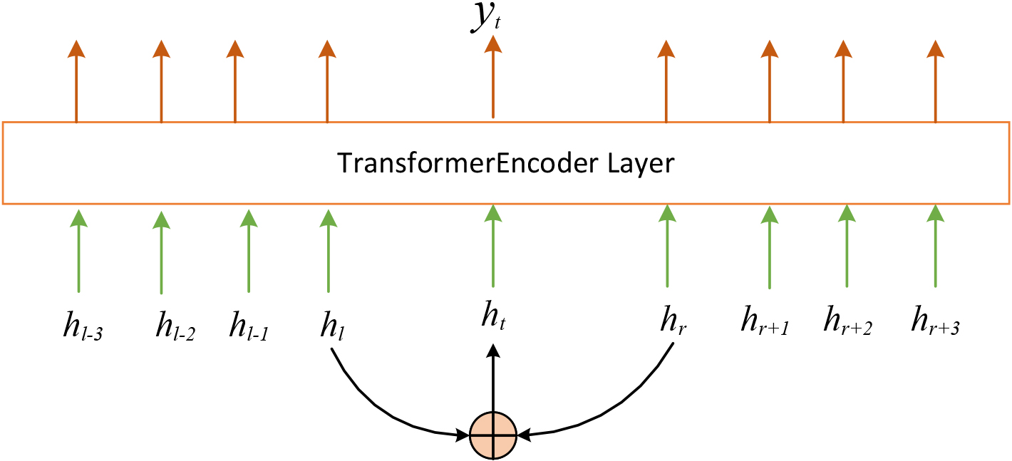

This paper only uses Transformer Encoder to process features, without considering the decoding function of the transformer. As shown in Fig. 6, after the six-layer coding process of the Transformer, the feature information in the past and the future can learn from each other and finally output the represented feature vector.

For translation tasks, the transformer uses location coding to identify the word location. In this paper, the number of nodes in each snapshot is unvarying, and the location of the nodes does not change, so it is meaningless to code the location. Motivated by this reference [32], it proposed the timing code replace the position code according to the length of the time sequence snapshot. Based on the Bochner theorem, the kernel function is obtained by using the Euler formula and Monte Carlo integration, as shown in Eq. (28).

$\displaystyle K({t_{1}},{t_{2}})\approx\frac{1}{d}\sum\limits_{i=1}^{d}{\cos({% w_{i}}}{t_{1}})\cos({w_{i}}{t_{2}})+\sin({w_{i}}{t_{1}})\sin({w_{i}}{t_{2}})$ (28)

where d is the feature dimension and w is the weight parameter of the feature vector. For this paper, as shown in Eq. (29), $\textit{linspace}(0,9,len)$ is an equal intervals sequence with a total number of len between 0 and 9. ts is the input multi-dimensional feature vector group, map_ts is the timing code of the same dimension of the output.

$\displaystyle\textit{map\_{ts}}=\cos\left(\frac{{ts}}{{{{10}^{\textit{linspace% (0,9,len)}}}}}\right)$ (29)

4.4 Decoder of two stream architecture

Motivated by reference [33], which proposed a novel two-stream framework to predict human behavior, the attributes of human joints are regarded as the characteristics of points, and the attributes of bones are regarded as the characteristics of edges. This paper proposes the second AGBLTE model to process the edge features. When the output edge results are obtained, we concatenate the point results and edge results, then the full connect network is used to implement the binary classification.

4.4.1 Input Multi-perspective edge features

Similar to the way of processing node features, the edge features are also quantified from the micro, meso, and middle perspectives to obtain multiple features of the edge data. After the AGA layer processing, the results are transferred to exBiLSTM as input parameters for further processing.

From the micro perspective, the similarity indices of static link prediction can be used to represent the features of the edge, such as the common neighbor (CN) index, preferential attachment index, Resource allocation index, etc. This paper uses the CN index to characterize the edge feature from a micro perspective. As shown in Eq. (30), we use first-order and second-order common neighbors both express the attribute of the edge, and $\lambda$ is the adjustment coefficient.

$\displaystyle g_{1}^{\prime}(i,j)=\textit{CN}(i,j)+\lambda\cdot\sum\limits_{z% \in\Gamma(i)\cap\Gamma(i)}{(\textit{CN}(i,z)+\textit{CN}(j,z)})$ (30)

From the meso perspective, the number of triangular motifs is used to characterize the edge feature. As shown in Eq. (31), the number of triangular motifs passing through the edge is a first-order attribute, the number of triangular motifs between the endpoints on both sides of the edge and the common neighbors is a second-order attribute, and $\lambda$ is adjustment coefficient.

$\displaystyle g_{2}^{\prime}(i,j)={M_{ij}}+\lambda\cdot\sum\limits_{z\in\Gamma% (i)\cap\Gamma(j)}{({M_{iz}}+{M_{jz}}})$ (31)

From the middle perspective, the influence of nodes is characterized by the centrality of the edge within the subgraph. First, the network is divided into communities, then the betweenness of the edges within the community is used to characterize the edge feature from the middle perspective. As shown in Eq. (32). The numerator represents the number of edges from node $s$ to node $t$ . Nodes $s$ , $t$ , $i$ and $j$ all belong to the same community.

$\displaystyle g_{3}^{\prime}(i,j)=\left.\sum\limits_{s,t\in V}\frac{{\sigma(s,% t|i,j)}}{{\sigma(s,t)}}\right|s,t,i,j\in{C_{k}}$ (32)

4.4.2 Feature fusion and Decoder layer

Any graph network can be described by nodes and edges. As shown in Fig. 7, the two stream networks based on the AGBLTE model for node data and edge data respectively, and the node stream results are coupled with the features of the AGA layer to ensure the stability of the final features. Based on the cosine similarity method, as shown in Eq. (33), the edge similarity is represented by the two endpoint vectors.

$\displaystyle\textit{cosine}(a,b)=\frac{{\textit{dot}(a,b)}}{{\textit{norm(a)*% norm(b)}}}$ (33)

where dot represents the inner product of two vectors, and nom represents the normalization of the vector.

Figure 7.

Schematic diagram of processing flow based on two stream network.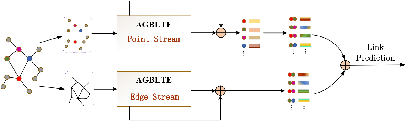

The AGBLTE processing of the edge stream is as same as that of the node stream. The output edge features are also coupled with the features of the AGA layer. Then they are further fused with the features of the node stream. As shown in Eq. (34), $\delta\in[0,1]$ is the adjustment coefficient between nodes and edges. The final similarity score after fusion is input to the full connect network for binary classification, and the temporal link prediction is realized according to the classification results.

$\displaystyle{S^{\textit{TSAGNN}}}=\delta\cdot\textit{Score\_point}+(1-\delta)% \cdot\textit{Score\_edge}$ (34)

5. Experiment

5.1 Datasets

This paper uses 8 real social network data sets and 1 randomly generated dynamic network data set to evaluate the performance. Email data set [34] is the email data of a large research institution in Europe. The WIKI dataset [34] contains the time series data of the user’s message operation on other users’ pages in Wikipedia. SXC2Q data set [34] is an interactive log on Math Overflow, an interactive mathematics website, which includes users’ questions, answers, comments, and other data. DNC data set [35] is the mail communication data collected in the mail leak incident of the Democratic National Committee of the United States; MAN dataset [35] is an e-mail record among employees in a manufacturing factory; LEM data set [36] The interactive event records collected by the US Kansas Event Data System, which contains the interactive information between Egypt, Israel, Jordan, Lebanon, Palestine, Syria, the US, and Russia. The IAEE dataset [37] consists of email data sent between Enron employees. SWE data set [38] is the network data selected by Wikipedia for voting and evaluation of administrators, reflecting the user’s approval or opposition to administrators. SBM dataset [16] is the dynamic network data generated by simulation using a random block model commonly used for community evolution simulation.

Table 1
Basic characteristic parameters of dataset

Dataset	Email	WIKI	SXC2Q	DNC	MAN	LEM	IAEE	SWE	SBM
Node number	1005	66,394	79,155	2,029	167	485	151	7,099	1000
Edge number	332,334	1,048,559	327,513	39,264	82,927	196,364	50,572	107,071	4,870,863
Start date	2003-10	2002-01-01	2009-09-30	2016-04-23	2010-01	1979-04	1999-05-11	2004-03-29	1
End date	2005-05	2008-01-06	2016-03-06	2016-05-25	2010-10	2004-06	2002-06-21	2008-01-06	50
Total duration	526 days	2196 days	2349 days	33 days	268 days	303 months	1137 days	1458 days	50
Temporal period	Week	Month	Month	Day	Week	Half a year	Month	Month	Once
Snapshot number	76	73	79	33	39	51	38	47	50

5.2 Baselines

(1)
GC-LSTM model [18]: This model embeds graph convolution network GCN into long short-term memory networks to achieve end-to-end dynamic link prediction. GCN can provide structure learning of network topology for each snapshot, while LSTM is responsible for time domain feature learning of each snapshot.
(2)
STGCN model [39]: This model combines the GCN and CNN into a function block for processing Spatial-temporal data. It can extract the most useful spatial features and continuously capture the most basic temporal features. It uses a bottleneck strategy to achieve scale compression and feature compression and uses a normalization function after each layer to prevent overfitting.
(3)
A3T-GCN model [40]: This model is also composed of multi-layer GCN and GRU, which can capture the global time dynamics information and spatial correlation information at the same time. GRU learns the short-term trend of time series, and GCN learning is based on the spatial dependence of network topology. The model also proposes the attention mechanism to adjust the importance of different sequence positions and integrates the global time information to improve prediction accuracy.
(4)
GConvLSTM model [15]: This model combines the Chebyshev convolutional network GCN based on the spectral domain with the LSTM is used to realize the temporal link prediction function of the dynamic network.
(5)
EvolveGCNO model [16]: This model uses GCN to process the information of the snapshots and uses the LSTM model to adjust the weight parameters of GCN, which could capture the dynamic features of the network.
(6)
LRGCN model [20]: This model is mainly used to deal with data’s temporal and spatial correlation. The model uses a two-layer GCN and attention mechanism to achieve the classification function of dynamic network data.
(7)
DynGEM model [24]: Based on static graph self-coding, this model minimizes the two objective functions corresponding to first-order approximation and second-order approximation and maps the input data to a highly nonlinear space to capture the evolution trend of the network.
(8)
DyGrEncoder model [41]: This model designs an unsupervised encoder-decoder framework, which projects the dynamic graph into multi-dimensional space at each time step, and simultaneously considers the topological structure features and evolution features of the network.
(9)
TREND model [42]: This model uses Hawkes process-based GNN to integrate with event and node dynamic features. It uses GNNs to materialize the temporal representations by receiving and aggregating messages of the node itself and the historical neighbors. It also integrates the event and node losses to jointly optimize event and node dynamics.
(10)
MLjFE model [43]: This model proposes a special case of a multi-label learning framework for temporal link prediction. It is developed for temporal link prediction by joint multi-label learning and feature extraction, where features can capture the information in a parameter matrix for temporal link prediction.

5.3 Results

The experimental running environment is 64-core Intel (R) Xeon (R) Gold 5218 CPU @ 2.30 GHz, NVIDIA Geforce RTX 3090 GPU, 256 GB memory. The Python version is 3.8.12, and the PyTorch version is 1.9.0. The learning rate parameter LR of the optimizer is 0.01, and the training parameter epoch of the model is 20. Since the large node number of some data sets such as WIKI, SXC2Q and SWE, we sample 3000 nodes from each dataset, which ensures that the sampled nodes and edges are partially occurrent at every moment. Set $\lambda=0.5$ , which is the adjustment coefficient of the second order neighbor in feature mapping processing; Set the parameters of the CABs in the AGA Layer as shown in Fig. 3, the first GCN output feature dimension is 48, the second GCN output feature dimension is 64, the first GAT output dimension is 128, drop $=$ 0.5, and the second GAT is the attention result of the single header; Set the hidden layer dimension of exBiLSTM is 128 and the output dimension is 32; Set $\delta=0.1$ , which is the adjustment parameters of node and edge features in the two-stream architecture; The hidden layer dimension of the full connect MLP of the decoder is 32, and the output dimension is 2. TSAGNN is a two-stream processing method based on three kinds of inputs, using TSAGNN_p refers to the ablation model using only node features, TSAGNN_e is used refers to the ablation model that only uses edge features, and TSAGNN_d used represents the ablation model with the same input features as the baseline methods. Since the neural network sets random discarding parameters in the process of feature transmission, the experimental results of all models have a performance deviation of about 0.03.

5.3.1 Comparison and analysis of prediction performance

GC-LSTM, STGCN, and A3T-GCN belong to the stacked GNN model. GConvLSTM, EvolveGCNO, and LRGCN belong to the integrated GNN model. DynGEM, DyGrEncoder, and TREND belong to the dynamic coding model. MLjFE belongs to the Matrix decomposition model. The input parameters of these models adopt a one-hot feature or degree matrix feature, we select the results with better effect for comparison. Set the train window size $p=$ 3, which chooses three historical snapshots to train. We randomly choose 30 snapshots to test and compare the average value of all evaluation results. The proposed method achieves the best prediction AUC, Brier, and MAP accuracy in nine data sets, and the results of RMSE and MAE are relatively better in most situations. The specific conclusions are as follows:

Table 2
AUC performance result table

Dataset	Email	WIKI	SXC2Q	DNC	MAN	LEM	IAEE	SWE	SBM
GCLSTM	0.5787	0.5583	0.6403	0.6134	0.6115	0.6000	0.7182	0.4501	0.6778
STGCN	0.8150	0.8145	0.8814	0.6805	0.7927	0.6229	0.8084	0.4273	0.7221
A3TGCN	0.8084	0.8046	0.8342	0.6858	0.7782	0.6698	0.8164	0.4208	0.7270
GConvLSTM	0.6324	0.7150	0.6413	0.5765	0.5842	0.5748	0.7472	0.3417	0.6325
EGCNO	0.6444	0.6397	0.7783	0.6824	0.5882	0.5220	0.7209	0.5986	0.6332
LRGCN	0.5707	0.6885	0.6589	0.6116	0.5964	0.6664	0.7193	0.4615	0.6515
DYNGEM	0.5310	0.5650	0.6965	0.5347	0.6973	0.6039	0.6427	0.5027	0.6306
DyGr	0.6467	0.7394	0.8713	0.6460	0.5577	0.5608	0.7479	0.4754	0.5863
TREND	0.6525	0.6213	0.7347	0.5937	0.6276	0.5862	0.7033	0.5136	0.6875
MLjFE	0.8458	0.8085	0.8588	0.7189	0.8349	0.7499	0.7604	0.6249	0.7519
TSAGNN	0.8762	0.8520	0.9067	0.7366	0.8878	0.8688	0.8706	0.7832	0.7890

Because the stacked GNN model has separately extracted the spatial features of the network topology at each moment, the effect of GCLSTM, STGCN, and A3TGCN in most datasets is better than that of the integrated model and dynamic coding model. The proposed TSAGNN model also uses the stacking method to process the features of each snapshot, and the input spatial information is more than the stacked GNN models. From Table 2, we can see that the effect of AUC has been significantly improved. Compared with the baseline methods with better prediction results, the performance of the method in nine datasets has been improved by 2% $\sim$ 29%, the effect in the LEM dataset has been improved mostly, and the average AUC has been improved by about 15%.

The integrated GNN model processes spatial and temporal information at the same time. The TSAGNN model also uses the way of the integrated method. While processing temporal information between each LSTM cell, GCN is also used to further process spatial information. The effect of the integrated model in the SWE dataset is better than that of the stacked model and the dynamic coding model. Similarly, the TSAGNN model has also achieved the best AUC effect, which makes an average improvement of more than 14%.

Moreover, the effect of the TSAGNN model is also significantly improved compared with DynGEM, DyGr, TREND, and MLjFE models, and the average improvement effect is between 4% and 30%.

Table 3

Brier performance result table

Dataset	Email	WIKI	SXC2Q	DNC	MAN	LEM	IAEE	SWE	SBM
GCLSTM	0.2842	0.2807	0.3853	0.2782	0.2776	0.2622	0.2381	0.2986	0.2953
STGCN	0.3360	0.2952	0.3205	0.3122	0.2672	0.3585	0.2912	0.3720	0.2863
A3TGCN	0.3120	0.2944	0.3491	0.3241	0.2919	0.3279	0.3368	0.3638	0.2789
GConvLSTM	0.2727	0.2604	0.3442	0.2995	0.2806	0.2768	0.2301	0.3319	0.2889
EGCNO	0.3416	0.4037	0.3067	0.3640	0.3701	0.4582	0.3680	0.4641	0.4507
LRGCN	0.2726	0.2781	0.3766	0.2922	0.2739	0.2646	0.2283	0.3032	0.3082
DYNGEM	0.3536	0.3529	0.4644	0.5121	0.3429	0.3459	0.3784	0.3957	0.3210
DyGr	0.4279	0.3719	0.3916	0.3395	0.3701	0.4487	0.2566	0.4635	0.2930
TREND	0.3475	0.3106	0.3745	0.3567	0.2901	0.4047	0.3453	0.4316	0.3388
MLjFE	0.2963	0.2741	0.2632	0.3156	0.3219	0.3923	0.2469	0.3078	0.3146
TSAGNN	0.2093	0.1587	0.1396	0.2239	0.1737	0.1596	0.1525	0.287	0.3098

The average Brier accuracy of the TSAGNN model has also been greatly improved in most datasets except SBM. As shown in Table 3, TSAGNN performs a little better in SWE, about 4% higher than the GC-LSTM model. For the other seven datasets, the average performance is improved by more than 30%.

Table 4

MAP performance result table

Dataset	Email	WIKI	SXC2Q	DNC	MAN	LEM	IAEE	SWE	SBM
GCLSTM	0.4958	0.6107	0.7460	0.6168	0.6069	0.5820	0.7427	0.4591	0.6315
STGCN	0.8139	0.8161	0.8978	0.6646	0.7797	0.6017	0.8276	0.4512	0.6506
A3TGCN	0.8031	0.8087	0.8716	0.6704	0.7620	0.6506	0.8453	0.4497	0.6548
GConvLSTM	0.5887	0.7323	0.7477	0.6066	0.5760	0.5629	0.7616	0.4018	0.6078
EGCNO	0.6035	0.6139	0.7311	0.6435	0.5626	0.5149	0.7027	0.5821	0.5984
LRGCN	0.5381	0.7071	0.7547	0.5498	0.5830	0.6547	0.7470	0.4767	0.6189
DYNGEM	0.5035	0.6298	0.7750	0.5308	0.6570	0.5711	0.6908	0.5077	0.6006
DyGr	0.6135	0.7599	0.8854	0.5568	0.5515	0.5385	0.7747	0.4885	0.6056
TREND	0.5967	0.6875	0.7349	0.5726	0.5997	0.6108	0.7594	0.5148	0.6716
MLjFE	0.8687	0.8045	0.6987	0.7323	0.8141	0.7165	0.7884	0.6632	0.7113
TSAGNN	0.8857	0.8737	0.9347	0.7972	0.8932	0.8826	0.8827	0.8311	0.7890

The average MAP accuracy of the TSAGNN model has also been greatly improved. As shown in Table 4, TSAGNN performs a little better in SXC2Q and IAEE, about 4% higher than the baseline models. For the other seven datasets, the average performance of TSAGNN has been greatly improved, which is about 2% $\sim$ 42%. It can be seen that the improvement effect of TSAGNN’s MAP index is significantly higher than others’ models.

Figure 8.

Schematic diagram of RMSE and MAE experimental results.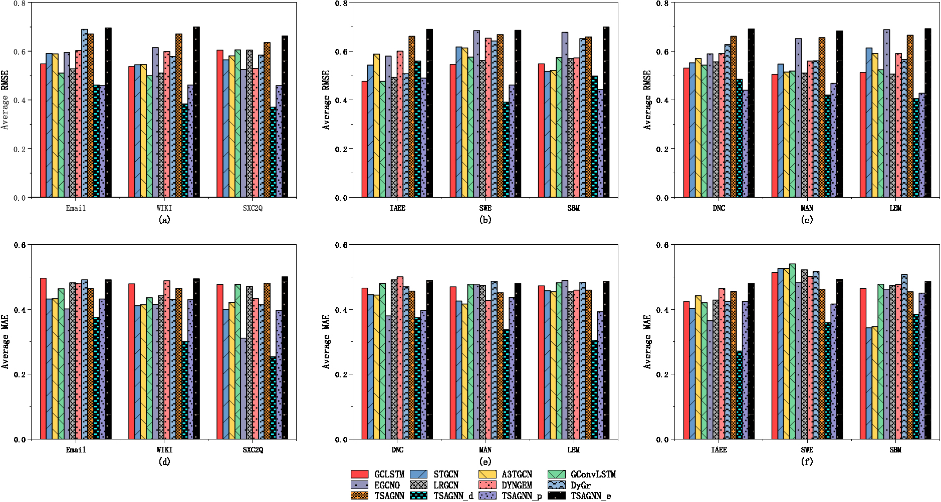

As shown in Fig. 8(a) (b) (c), the result is the test comparison of the RMSE effect in nine data sets. The error of the TSAGNN and TSAGNN_e are relatively bigger in the experiment. Except that the RMSE of GCLSTM and GConvLSTM in the IAEE dataset is the minimum value, TSAGNN_p and TSAGNN_d have achieved better results in other cases. The average RMSE of the TSAGNN_d is reduced by more than 10%. When the same features are inputted, the better results of the TSAGNN_d show that the design of the two-stream graph neural network processing layers and the transformer encoder has better RMSE performance.

Similarly, as shown in Fig. 8(d) (e) (f), it is the experimental comparison results of the MAE effect in nine data sets. TSAGNN_d in other data sets except the SBM data set is relatively better, and the average of MAE is reduced by more than 15%. The MAE performance of the TSAGNN_p is better than TSAGNN_e and TSAGNN, which indicates the processing of edge features may make a bigger error result.

Figure 9.

Schematic diagram of input characteristic sensitivity test. (a) Comparison of ablation model results with different input characteristics. (b) Comparison of graph network results with different layers.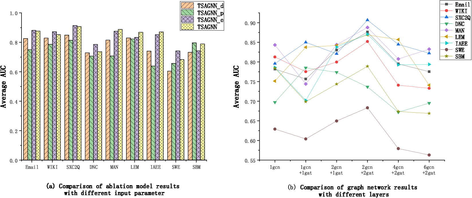

5.3.2 Sensitivity testing of input parameters

First, we test the performance of different input features and compare TSAGNN_d, TSAGNN_p, TSAGNN_e, and TSAGNN. As shown in Fig. 9(a), the AUC effect of TSAGNN is better than the TSAGNN_d in all nine data sets, which indicates the more features that can be input, the better performance can be gotten. The average improvement effect is about 7%. And in the SBM dataset, TSAGNN_p based on point features could get better results, and the results of TSAGNN_e based on edge features in other datasets are better, which indicates the fusion of node features and edge features can better improve the prediction performance in different network environments.

Moreover, the CABs of the AGA layer are used to process the input information using multi-layer neural networks, and the influence of different neural network structures on the AUC performance is tested. We test the 1-layer GCN network, the 1-layer GCN and 1-layer GAT network, the 1-layer GCN and 2-layer GAT network, the 2-layer GCN and 2-layer GAT network, the 4-layer GCN and 2-layer GAT network, the 6-layer GCN and 2-layer GAT network respectively. The average AUC results are shown in Fig. 9(b). while the optimal situation occurs in the 1-layer GCN+1gat mode in the DNC data, the best case in other data sets is 2gcn+2gat. The AUC effect of the 4gcn+2gat and 6gcn+2gat drop sharply, which indicates the more layers of the neural networks, the effect of the performance may be worse. According to the experimental results, it is suggested that the number of layers for setting CABs should not exceed 4 and that 2-layer GCN and 2-layer GAT networks can achieve the best processing results in most situations.

5.3.3 Temporal robustness

According to the total size of the snapshots of different datasets, we choose 20–30 consecutive target snapshots for testing to observe the prediction effect of different methods. As shown in Fig. 10, the TSAGNN method has improved the prediction effect at most times in nine data sets, and the AUC curve has higher performance and stability at different moments. In contrast, the prediction accuracy of other baseline methods decreases greatly at some time, the AUC curve of them fluctuates greatly, and the average AUC is significantly lower than TSAGNN. The above results verify that TSAGNN has better temporal robustness in dynamic network link prediction tasks.

Figure 10.

Schematic diagram of AUC performance with different methods changing in time sequence.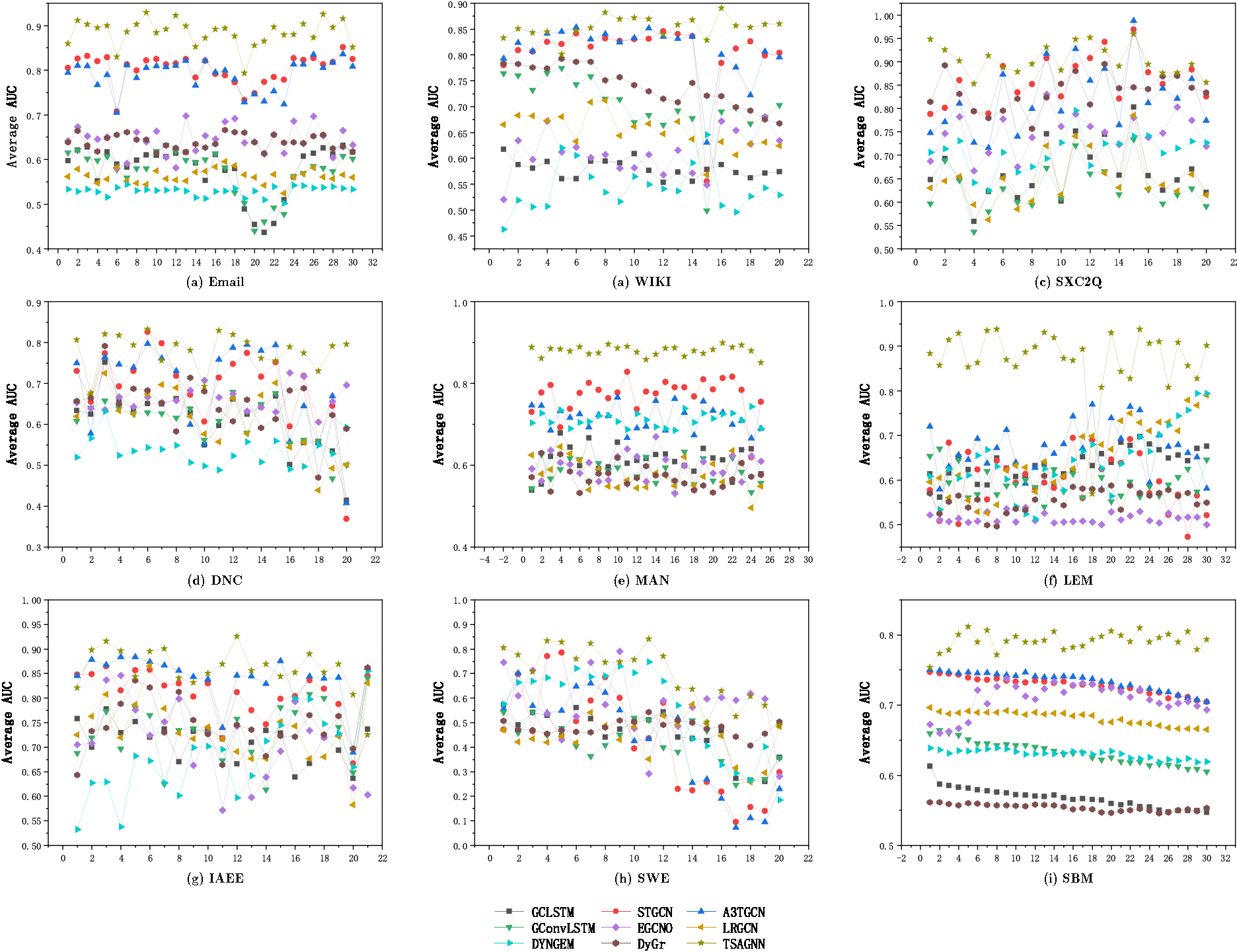

6. Conclusions

In this paper, we research the temporal link prediction problem of dynamic networks based on graph neural networks. At present, many graph neural networks often use one-hot feature or label features as the original input, they do not consider the diverse scenarios of input feature parameters, and the utilization of time-domain features and spatial-domain features is limited. To solve these problems, a novel temporal link prediction method based on two streams of adaptive graph neural networks is proposed, which can fully mine the spatial and temporal information of the dynamic network. Firstly, we propose an adaptive mechanism that combines convolutional neural networks and self-attention networks for the spatial features of different scale network structures. Secondly, an extended bi-directional long short-term memory network is proposed, which uses graph convolution to process topological features, and recursively trains the time-domain memory information. Thirdly, the location coding is replaced by the time-coding for the transformer encoder, so that the past information and the future information can be learned from each other, and the time-domain information of the network can be further mined. Furthermore, a two-stream network framework is proposed, which combines the processing results of point features and edge features, and the fully connected network for decoding to realize the temporal link prediction. Finally, the experimental results on 9 network datasets show that the proposed method has a better prediction effect and better robustness than the classical graph neural network methods under the AUC, Brier, MAP, RMSE, and MAE metrics. The follow-up research problem in the future is how to predict and reconstruct multi-layer networks, self-organizing networks, weighted networks, and continuous networks with various dynamic spatial-temporal information.

Footnotes

Acknowledgments

This research was supported by the National Natural Science Foundation of China (No.61803384).

References

Stankovic

Mandic

Dakovic

Brajovic

Scalzo

Constantinides

, Graph Signal Processing–Part I: Graphs, Graph Spectra, and Spectral Clustering, arXiv preprint arXiv:1907.03467, (2019).

Mohan

Pramod

, Link prediction in dynamic networks using time-aware network embedding and time series forecasting, Journal of Ambient Intelligence and Humanized Computing 12(2) (2021), 1981–1993.

Holme

Saramaki

, Temporal Network Theory 8 (2019), 375.

Güneş

İ.

Gündüz-Öğüdücü

Ş.

Çataltepe

, Link prediction using time series of neighborhood-based node similarity scores, Data Mining and Knowledge Discovery 30(1) (2016), 147–180.

Perozzi

Al-Rfou

Skiena

, Deepwalk: Online learning of social representations, in: Proceedings of the 20th ACM SIGKDD international conference on Knowledge discovery and data mining, New York, USA, 2014, pp. 701–710.

Grover

Leskovec

, node2vec: Scalable feature learning for networks, in: Proceedings of the 22nd ACM SIGKDD international conference on Knowledge discovery and data mining, 2016, pp. 855–864.

Tang

Wang

Zhang

Yan

Mei

, Line: Large-scale information network embedding, in: Proceedings of the 24th international conference on world wide web, 2015, pp. 1067–1077.

Skarding

Gabrys

Musial

, Foundations and modeling of dynamic networks using dynamic graph neural networks: A survey, IEEE Access 9 (2021), 79143–79168.

Bouarara

H.A.

, Recurrent neural network (RNN) to analyse mental behaviour in social media, International Journal of Software Science and Computational Intelligence (IJSSCI) 13(3) (2021), 1–11.

10.

Liu

Yin

Song

, K-core based temporal graph convolutional network for dynamic graphs, IEEE Transactions on Knowledge and Data Engineering (2020).

11.

Manessi

Rozza

Manzo

, Dynamic graph convolutional networks, Pattern Recognition 97 (2020), 107000.

12.

Veličković

Cucurull

Casanova

Romero

Lio

Bengio

, Graph attention networks, arXiv preprint arXiv:1710.10903, (2017).

13.

Zhang

Shi

Xie

King

Yeung

D.-Y.

, Gaan: Gated attention networks for learning on large and spatiotemporal graphs, arXiv preprint arXiv:1803.07294, (2018).

14.

Sankar

Gou

Zhang

Yang

, Dysat: Deep neural representation learning on dynamic graphs via self-attention networks, in: Proceedings of the 13th international conference on web search and data mining, 2020, pp. 519–527.

15.

Seo

Defferrard

Vandergheynst

Bresson

, Structured sequence modeling with graph convolutional recurrent networks, in: International conference on neural information processing, Springer, 2018, pp. 362–373.

16.

Pareja

Domeniconi

Chen

Suzumura

Kanezashi

Kaler

Schardl

Leiserson

, Evolvegcn: Evolving graph convolutional networks for dynamic graphs, in: Proceedings of the AAAI Conference on Artificial Intelligence, Vol. 34, 2020, pp. 5363–5370.

17.

Wang

Long

Wang

Gao

P.S.

, Predrnn: Recurrent neural networks for predictive learning using spatiotemporal lstms, Advances in Neural Information Processing Systems 30 (2017).

18.

Chen

Wang

, Gc-lstm: Graph convolution embedded lstm for dynamic link prediction, Applied Intelligence (2021).

19.

Schlichtkrull

Kipf

T.N.

Bloem

Berg

R.v.d.

Titov

Welling

, Modeling relational data with graph convolutional networks, in: European semantic web conference, Springer, 2018, pp. 593–607.

20.

Han

Cheng

Wang

Zhang

Pan

, Predicting path failure in time-evolving graphs, in: Proceedings of the 25th ACM SIGKDD International Conference on Knowledge Discovery & Data Mining, 2019, pp. 1279–1289.

21.

Jin

Jiang

Chen

Zhang

Szekely

Ren

, Recurrent event network: Global structure inference over temporal knowledge graph (2019).

22.

Bonner

Atapour-Abarghouei

Jackson

P.T.

Brennan

Kureshi

Theodoropoulos

McGough

A.S.

Obara

, Temporal neighbourhood aggregation: Predicting future links in temporal graphs via recurrent variational graph convolutions, in: 2019 IEEE international conference on big data (Big Data), IEEE, 2019, pp. 5336–5345.

23.

Rahman

Saha

T.K.

Hasan

M.A.

K.S.

Reddy

C.K.

, Dylink2vec: Effective feature representation for link prediction in dynamic networks, arXiv preprint arXiv:1804.05755 (2018).

24.

Goyal

Chhetri

S.R.

Mehrabi

Ferrara

Canedo

, Dynamicgem: A library for dynamic graph embedding methods, arXiv preprint arXiv:1811.10734 (2018).

25.

Chen

Zhang

Xuan

, E-lstm-d: A deep learning framework for dynamic network link prediction, IEEE Transactions on Systems, Man, and Cybernetics: Systems 51(6) (2019), 3699–3712.

26.

Hamilton

Ying

Leskovec

, Inductive representation learning on large graphs, Advances in neural information processing systems 30 (2017).

27.

Hajiramezanali

Hasanzadeh

Narayanan

Duffield

Zhou

Qian

, Variational graph recurrent neural networks, Advances in Neural Information Processing Systems 32 (2019).

28.

Peng

Liu

Weng

, Temporal link prediction in directed networks based on self-attention mechanism, Intelligent Data Analysis 26(1) (2022), 173–188.

29.

Divakaran

Mohan

, Temporal link prediction: A survey, New Generation Computing 38(1) (2020), 213–258.

30.

ZHU

LIU

, A Temporal Link Predict Algorithm Based on Fusion Local Structure Influence, Journal of Electronics & Information Technology 44(4) (2022), 1440–1452.

31.

Vaswani

Shazeer

Parmar

Uszkoreit

Jones

Gomez

A.N.

Kaiser

Ł.

Polosukhin

, Attention is all you need, Advances in neural Information Processing Systems 30 (2017).

32.

Ruan

Korpeoglu

Kumar

Achan

, Inductive representation learning on temporal graphs, arXiv preprint arXiv:2002.07962 (2020).

33.

Shi

Zhang

Cheng

, Two-stream adaptive graph convolutional networks for skeleton-based action recognition, in: Proceedings of the IEEE/CVF conference on computer vision and pattern recognition, 2019, pp. 12026–12035.

34.

Paranjape

Benson

A.R.

Leskovec

, Motifs in temporal networks, in: Proceedings of the tenth ACM international conference on web search and data mining, 2017, pp. 601–610.

35.

Kunegis

, Konect: the koblenz network collection, in: Proceedings of the 22nd international conference on world wide web, 2013, pp. 1343–1350.

36.

Batagelj

Mrvar

, Pajek datasets, 2006.

37.

Rossi

Ahmed

, The network data repository with interactive graph analytics and visualization, in: Twenty-ninth AAAI conference on artificial intelligence, 2015.

38.

Leskovec

Huttenlocher

Kleinberg

, Signed networks in social media, in: Proceedings of the SIGCHI conference on human factors in computing systems, 2010, pp. 1361–1370.

39.

Yin

Zhu

, Spatio-temporal graph convolutional networks: A deep learning framework for traffic forecasting, arXiv preprint arXiv:1709.04875 (2017).

40.

Bai

Zhu

Song

Zhao

Hou

, A3t-gcn: Attention temporal graph convolutional network for traffic forecasting, ISPRS International Journal of Geo-Information 10(7) (2021), 485.

41.

Taheri

Berger-Wolf

, Predictive temporal embedding of dynamic graphs, in: Proceedings of the 2019 IEEE/ACM International Conference on Advances in Social Networks Analysis and Mining, 2019, pp. 57–64.

42.

Wen

Fang

, Trend: Temporal event and node dynamics for graph representation learning, in: Proceedings of the ACM Web Conference 2022, 2022, pp. 1159–1169.

43.

Tan

Xie

Zhong

Deng

, Joint multi-label learning and feature extraction for temporal link prediction, Pattern Recognition 121 (2022), 108216.

TSAGNN: Temporal link predict method based on two stream adaptive graph neural network

Abstract

Keywords

1. Introduction

3. Preliminary

3.1 Problem definition

4.4.1 Input Multi-perspective edge features

5.1 Datasets

Table 1 Basic characteristic parameters of dataset

5.3.1 Comparison and analysis of prediction performance

Table 2 AUC performance result table

5.3.3 Temporal robustness

Footnotes

Acknowledgments

References

Table 1
Basic characteristic parameters of dataset

Table 2
AUC performance result table