Sage Journals: Discover world-class research

Abstract

The quest for transparency in black-box models has gained significant momentum in recent years. In particular, discovering the underlying machine learning technique type (or model family) from the performance of a black-box model is a real important problem both for better understanding its behaviour and for developing strategies to attack it by exploiting the weaknesses intrinsic to the learning technique. In this paper, we tackle the challenging task of identifying which kind of machine learning model is behind the predictions when we interact with a black-box model. Our innovative method involves systematically querying a black-box model (oracle) to label an artificially generated dataset, which is then used to train different surrogate models using machine learning techniques from different families (each one trying to partially approximate the oracle’s behaviour). We present two approaches based on similarity measures, one selecting the most similar family and the other using a conveniently constructed meta-model. In both cases, we use both crisp and soft classifiers and their corresponding similarity metrics. By experimentally comparing all these methods, we gain valuable insights into the explanatory and predictive capabilities of our model family concept. This provides a deeper understanding of the black-box models and increases their transparency and interpretability, paving the way for more effective decision making.

Keywords

Machine learning family identification adversarial black-box surrogate models

1. Introduction

The increasing ubiquity of machine learning (ML) models in devices, applications, and assistants, which replace or complement human decision making, is prompting users and other interested parties to model what these ML models are able to do, where they fail, and whether they are vulnerable [1]. However, many ML models are proprietary or black-box, with their inner workings inaccessible to users for confidentiality and security reasons. This is the case of FICO or credit score models, health, car, or life insurance application models, IoT Systems Security, medical diagnoses, facial recognition systems, etc. While publicly available query interfaces provide access to these models, they can also be exploited by attackers who can use ML techniques to learn about the behaviour of the model by querying it with selected inputs. This raises the issue of adversarial machine learning [2, 3] where the model’s intrinsic flaws and vulnerabilities are exploited to evade detection or game the system. In such scenarios, the attacker can gain an advantage by knowing the ML family and the true data distribution used to generate the attacked model.

Figure 1.

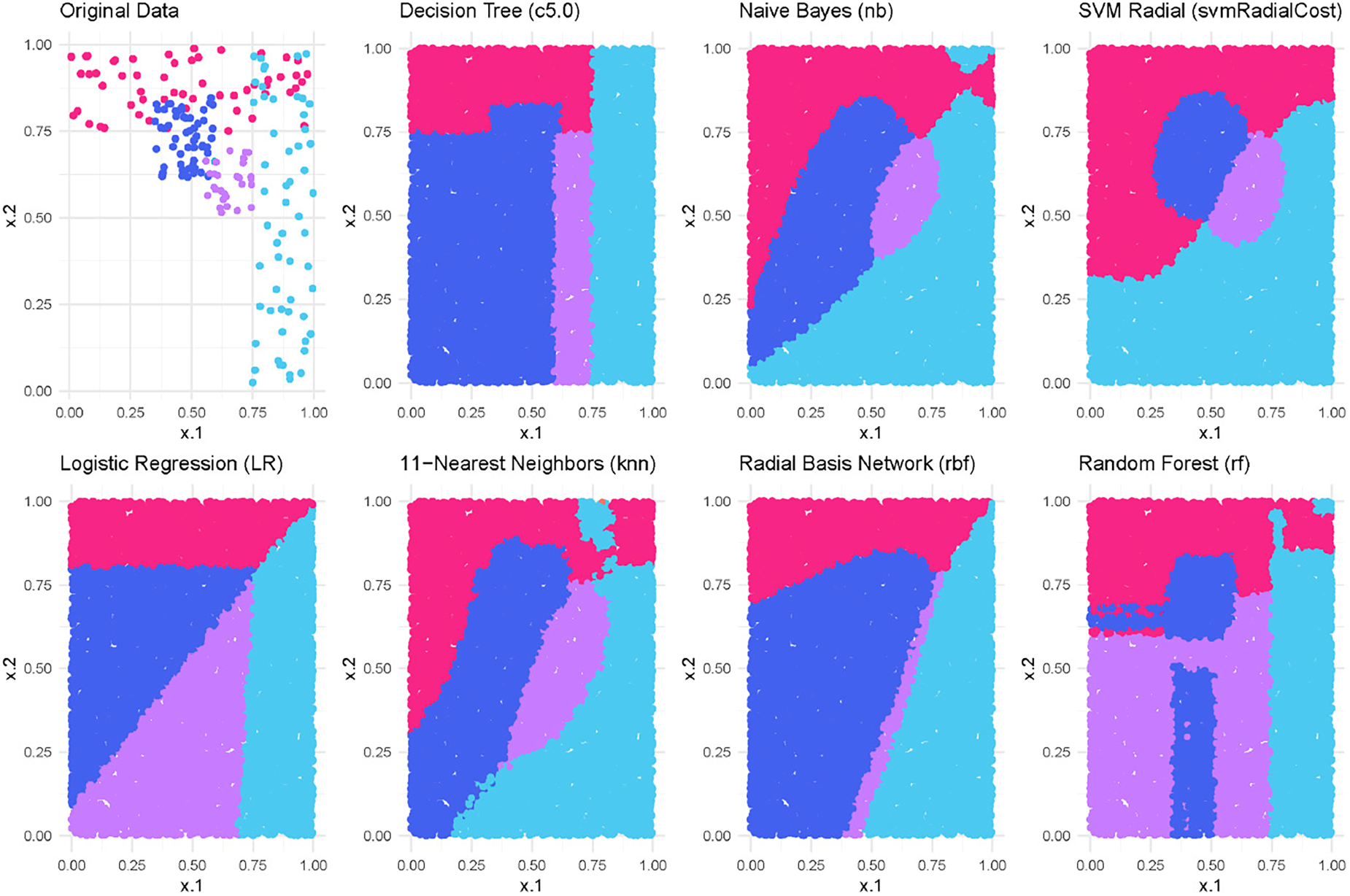
Behaviour of different models trained over the same four-class classification dataset (shown on the top-left plot). The pictures show the different prediction for particular class regions (known as decision boundaries) in dense and sparse areas.

One of the main reasons for not having general techniques for exploiting black-box models may be due to the intrinsic differences between ML techniques. Different models generated by specific machine learning techniques may differ not only in their decision boundaries, which are hypersurfaces that divide the input space into distinct classification regions, but also in their method of extrapolation in regions with few or no training examples. This is illustrated in Figure 1, where the top left plot shows the original training data of a bivariate dataset used to train several machine learning models using different techniques. The observation here is that all models show similar behaviour, i.e. they produce comparable partitions of the input space in densely populated zones where the training examples are located. However, their behaviour in areas with sparse or no training examples tends to be unpredictable and highly dependent on the specific ML technique employed. Recognising the distinctive decision-making characteristics of different ML families is fundamental to the aims of this paper [4, 5]. In particular, these less densely populated zones are more prone to error. Given the different ways in which different model families extrapolate within these sparse regions, specific strategies have been developed to attack, extract and steal machine learning models belonging to particular families, such as Support Vector Machines [6], (Deep) Neural Networks [7], Naive Bayes [8], and even various online prediction APIs [9]. Knowing the model’s family can thus help predict its vulnerabilities and promote more comprehensive defence strategies against adversarial attacks [10, 11].

ML family identification also holds importance across various domains that benefit from understanding model behaviour, especially in areas with sparse or no training data. This is particularly relevant for Open Set Recognition [12] and Novelty Detection [13], where the goal is to detect unseen classes or categories that were not present during the model’s training phase. Similarly, in outlier and anomaly detection [14, 15], identifying sparse classes within the training data is a major challenge. In addition, understanding the ML family is critical to meeting the legal and ethical requirements of AI deployment [16]. Knowledge of the ML family serves as a key measure of transparency, potentially satisfying regulatory requirements and preemptively addressing ethical concerns.

In this paper, we address the problem of experimentally determining the machine learning technique family that was used for training a model that is presented as a black-box model. Unveiling the family of a model, if possible, could be seen as the initial step for an adversarial learning procedure. Once we have some knowledge of the ML family used in the model, we can apply specific adversarial techniques tailored to that family, such as those mentioned above. Our aim is to address this issue in a realistic context where our ability to make queries is not unlimited, and we assume that we lack any information about the model, including the learning algorithm used for training, as well as the original data distribution. Our goal is not to duplicate the machine learning model or to identify the full hypersurface that divides the feature space. Instead, we seek to identify the specific machine learning technique by using queried input-output pairs. This technique should exhibit behaviour that closely mirrors the behaviour manifested by the black box model across the data space.

Our approach considers the black-box model as an oracle for labelling a synthetic dataset generated by following a specific query strategy. This approach is particularly useful when we have no information about the black-box model or its training data distribution, as is often the case in real-world applications. This artificial dataset serves as the basis for training different models, each of which uses different machine learning techniques from different learning families to approximate the behaviour of the oracle. These models are called surrogate models. We propose two methods to identify the ML family of the oracle based on the (dis)agreement between the decisions made by the oracle and each surrogate model. The first is the crisp scenario, where the oracle only provides the class label for each example. That is, it returns a qualitative value indicating the predicted class among the possible categories, without any additional information. This scenario includes all cases where the output of the oracle is strictly limited to these class labels. The second one is called the soft scenario, characterised by the fact that the oracle provides class probability estimates along with the class labels. These are essentially confidence scores for each class, adding a layer of quantitative judgement to the prediction. The soft scenario plays a key role in applications where it is essential to have predictions in the form of scores or probabilities rather than just class labels. Examples of such applications include weather forecasting [17, 18], where predictions may be accompanied by a percentage chance of occurrence; betting-based forecasting [19, 20], which relies on probability estimates to make decisions; or sentiment analysis tools [21, 22], which quantify the sentiment expressed in text data. These scenarios require a more nuanced understanding of predictions, making the soft scenario particularly relevant.

The structure of our paper is as follows. Section 2 provides a brief overview of related work. In Section 3, we present our approach for predicting the ML family of a black-box model. The experimental evaluation is discussed in Section 4. Lastly, we conclude our paper in Section 5, where we summarize our findings and outline directions for future research.

2. Related work

In this section, we review the literature related to the learning from queries labelled by an oracle (human or ML model) and approaches to interpretable machine learning that rely on learning a substitute model for explaining the decisions of any model.

There is extensive literature on the topic of learning from queries labelled by an oracle or an expert. Examples can be found in the fields of learning theory [23, 24], concept learning [25, 26, 27], learning of regular sets [25], and active learning [28, 29]. In all these cases, it is assumed that the information about the data distribution is given in order to generate the queries about the concept to be learned.

The area of adversarial machine learning [30, 31, 32, 33]has addressed the task of learning from queries labelled by a model (the oracle) but with the aim of attacking it [34]. Thus, the queries are used to capture information about the decision layouts of the model to be attacked trying to discover its vulnerabilities. To this aim, several specific query strategies exist depending on the type of model to be attacked, for instance, support vector machines [6], or deep neural networks [7, 35, 36, 37, 38].

Different query-based methods have been introduced to explain and replicate the behaviour of an incomprehensible model. A simple way to capture the semantics of a black-box ML model consists of mimicking it to obtain an equivalent one. This can be done by considering the model as an oracle and querying it with new synthetic input examples (queries) that are then labelled by the oracle and used for learning a new declarative model (the mimic model) that imitates the behaviour of the original one. Domingos et al. [39] addressed this problem by creating a comprehensible mimetic model (decision trees) from an ensemble method. Blanco-Vega et al. analysed the effect of the size of the artificial dataset in the quality of the replica and the effect of pruning the mimetic model (a decision tree) on its comprehensibility [40], developing also an MML-based strategy [41] to minimise the number of queries. Papernot et al. [10] also applied a mimicking strategy but for adversarial purposes. The idea is to create a replica of the original black-box model aiming at crafting examples on the basis that the examples that affect one model also affect any other model trained for the same task. More recently, Yang et al. [42] presented a query black-box based attack method that adapts the surrogate model by constructing a high-gradient computation graph, in order to approximate the surrogate model to the oracle model, in both forward and backward pass.

Another related area is ‘interpretable machine learning’ [4] (or the broader ‘explainable AI’, XAI [43]) which aims at making machine learning models and their decisions more interpretable. In this field, black-box models are described by considering aspects like feature importance, accumulated local effects, or addressing the justification of individual predictions. A popular work is LIME [44], a technique that explains a prediction of any classifier by learning an interpretable linear model locally around the prediction. Similarly, LORE [45] explains specific predictions of a classifier by learning an interpretable model locally to the instance, providing a rule and a set of counterfactual rules. Recently, Maaroof et al. [46] extended the LORE method to explain the decisions of multi-class fuzzy-based classifers.

Our proposal differs from the previous approaches in that we do not aim to replicate the black-box model, nor to determine the full decision boundary that partitions the feature space. Instead, our focus is on identifying important features of the model, such as its ML family, which can serve as a crucial first step before applying more specific adversarial techniques. To achieve this goal, we treat the black-box model as an oracle and generate a set of synthetic input examples to be labelled by the oracle. Our approach also differs from the traditional mimetic method in that we use the labelled artificially-generated input examples (by assuming no prior knowledge of the original model or training data) to train multiple surrogate models using different ML techniques with the aim of approximating the behaviour of the black-box model. By comparing the decisions made by the oracle and each surrogate model, we can identify the ML family of the black box model. This approach is particularly useful in scenarios where the original model is proprietary or confidential, and there is no access to information about the learning algorithm or the original data distribution. Another approach also based on the idea of using examples labelled by a black-box model to discover some of its proprietary properties has been explored in [47], but with the goal of finding out some properties of neural networks such as the type of activation, the optimisation process and the training data.

3. Model family identification

As we discussed in Section 1, the behaviour of a model depends on, among other factors, the ML technique applied to learn the model. Hence, one way of determining the ML family of a black-box model could be to mimic it trying to approximate the nature of the decision boundaries. One way of doing this is to create different surrogate models using techniques from different learning families and input-output pairs generated by the original black-box model as an oracle. We can then compare the decisions made by each surrogate model with those made by the original oracle, using an appropriate measure of agreement/discrepancy or disagreement.

3.1 Generating surrogate models

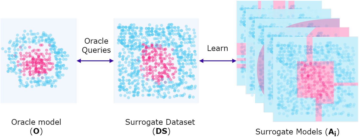
A black-box model can act as an oracle, denoted $O$ , which can be queried to obtain its predictions. Depending on the nature of the oracle, either only class labels or class membership probabilities can be obtained, resulting in a crisp or soft classifier. Using this, an artificial dataset can be created and labelled by $O$ , which we call the surrogate datasetSD. In this way, SD is able to capture the decision patterns of $O$ as well as the class distribution inferred by $O$ . Figure 2 illustrates the process.

Figure 2.

A black-box model (oracle) trained on an unknown original dataset acts as a source of labels for synthetic surrogate datasets. These synthetic datasets are generated by following specific query strategies designed to capture the decision-making process of the black-box model. The surrogate dataset (SD) is then used to train multiple surrogate models, each using a different machine learning technique. The goal is to approximate the behaviour of the black-box model without having access to its original data distribution or the specific learning algorithm used to train it.

The generation of synthetic examples to interrogate the black box model $O$ can be achieved by various strategies. A viable approach is to assume feature independence, which is the only logical assumption in the absence of the original input data, and then generate random values for each feature. These values are generated within plausible attribute bounds, following the uniform distribution (We have also experimented with alternative querying strategies, such as the Uniform Grid [48] approach, where samples are generated using node points at fixed intervals uniformly distributed for every dimension. However, this strategy resulted in poorer performance due to inadequate input coverage in datasets with low sampling points and high dimensions, and also had efficiency issues). This method provides good coverage of the feature space, especially in non-dense regions where the behaviour of $O$ is likely to be unexpected, revealing potential vulnerabilities. It is important to recognise that differences between model families, particularly in the distribution of class labels within the feature space, are more pronounced in less dense regions. This includes regions where queries may not even be relevant, as shown in Figure 1. Therefore, this query strategy seems well suited to the goal of finding the ML family of $O$ .

The artificial inputs, paired with the class labels predicted by $O$ , form the surrogate data set, denoted SD. By using SD for training, we are able to develop different surrogate models, each of which reflects the behaviour of $O$ to a different degree. Specifically, given SD and a set of $N$ families of machine learning techniques, a surrogate model $A_{i}$ is developed for each ML family $i \in N$ . Consequently, each surrogate model $A_{i}$ can provide a unique characterisation of SD and, by extension, insight into the characteristics of $O$ . The process is illustrated in Figure 2.

3.2 Measuring similarity between models

To identify the family of the oracle, it is necessary to use evaluation measures that estimate the similarity between the surrogate models and the oracle with respect to a given dataset. In the case of the crisp scenario, where the classifiers predict class labels, Cohen’s kappa coefficient ( $κ$ ) [49] can be used as it estimates the inter-rater agreement for qualitative items. The kappa coefficient takes into account not only the number of agreements and disagreements, but also the agreement that could occur by chance. This makes it a more reliable measure than a simple percentage of agreement, especially when dealing with unbalanced datasets where the majority class may dominate the agreement metric [50]. Furthermore, in our approach we use the kappa coefficient to compare how different classifiers agree or disagree on boundaries caused by extrapolation to sparse areas when explaining the same dataset SD, which can be obtained using a train-test split or cross-validation. Therefore, a $κ_{i}$ value can be calculated for each surrogate model $A_{i}$ . Figure 3 illustrates the process.

Figure 3.

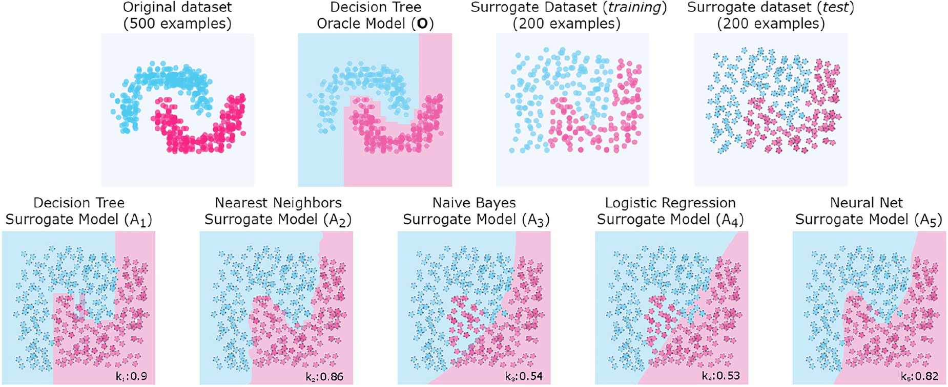
Synthetic example to show the $κ$ measure for different surrogate models $A_{i}$ when compared to an specific oracle model $O$ learned by using a decision tree technique. The bottom row includes the surrogate models inferred from the training SD (background colors) and its performance on the test SD with the $κ$ value. Note that surrogate models are trained from a non-linearly separable data and, thus, models producing linear boundaries such as the logistic regression or Naïve Bayes cannot emulate a quadratic decision boundary which is required.

At the top of the Figure 3 we see (from left to right) the original dataset, the oracle model $O$ , the surrogate training set (SD) and the test set (these two sets are labelled with $O$ ). The training set SD is used to learn all the surrogate models $A_{i}$ shown in the bottom row. The test set is used to evaluate each of the $A_{i}$ (i.e. to obtain each $κ_{i}$ score). It is easy to see that the surrogate model whose decision boundaries are most similar to those of $O$ is the decision tree (bottom left plot), as confirmed by its kappa value ( $κ_{1} =$ 0.90), although some other techniques also do a good job (e.g. nearest neighbours). The surrogate decision tree has more in common with the oracle than with other models because they both have high expressiveness with boundaries that are always parallel to the axes. This similarity is due to the fact that, despite possible differences in the specific techniques used to develop them, they come from the same family of models. Regarding the nearest neighbour model, despite its high expressiveness, its boundaries are clearly not parallel to the axes, showing a sawtooth pattern that would be particularly difficult to replicate using decision trees. This discrepancy is indicated by a lower $κ$ value. Other surrogate models, such as logistic regression or Naïve Bayes, which are less powerful, give significantly worse results, as can be seen either visually or through the $κ$ measure.

As mentioned above, the way different families of models extrapolate decision boundaries can vary significantly depending on several factors, such as overfitting, underfitting or generalisation. In addition, such factors depend on the characteristics of the original dataset, such as noise, sparsity, or separability. For example, logistic regression and Naïve Bayes models can produce similar decision bounds for a linearly separable dataset. However, if the dataset is not linearly separable (as shown in Figure 3), other learning techniques can produce similar boundaries, such as decision trees, nearest neighbours, and even neural networks. However, we have no prior knowledge of the original dataset used to train the oracle. We do not know the sparsity, separability, or any other property that might be relevant to accurately identify the family of models. Hence, it is convenient to compare the behaviour of the oracle with a variety of surrogate models from different learning families to increase the likelihood of correctly identifying the original model family.

3.3 Maximum similarity approach

In the example in Figure 3, we observed that the family of the oracle model $O$ was the one that achieved the highest $κ$ among the surrogate models $A_{i}$ . This suggests our first approach to family identification, which we call the maximum similarity. Generally speaking, this approach consists of identifying the surrogate model $A_{i}$ that has the most similar behaviour to $O$ according to a certain similarity measure, and then considering the family of $O$ to be the same as the family of $A_{i}$ . In what follows, we specify this approach for each of the scenarios considered in this work.

3.3.1 Crisp classifiers

In the scenario where both the oracle and the surrogate models are crisp classifiers, identifying the ML family of the oracle is relatively straightforward. We first evaluate the surrogate dataset SD with the different surrogate models $A_{i}$ , each belonging to a different ML family $i \in N$ , using Cohen’s Kappa metric. Then we assign the oracle to the ML family of the surrogate model $A_{i}$ that has the highest $κ$ value, that is shown in Eq. (1).

\begin{aligned} F_{MS} (O) = {a r g m a x}_{i \in {1, \dots, N}} κ_{A_{i}} (SD) \end{aligned}

(1)

3.3.2 Soft classifiers

In the scenario where the oracle and surrogate models are soft classifiers, we cannot use Cohen’s kappa metric because it is only applicable to crisp classifiers. Instead, we need to measure the difference between the class probability vectors estimated by $O$ and those estimated by each surrogate model $A_{i}$ . To do this, we compute the error of the model $A_{i}$ as the difference between the predicted class membership probabilities given by $O$ and $A_{i}$ for SD. In this paper, we use the L1 norm (also known as the absolute error, AE) as a metric to measure the difference between the predictions. The L1 norm also provides some insight into how similar $O$ and $A_{i}$ distribute the class probabilities along the feature space.

To quantify the similarity in behaviour between $O$ and $A_{i}$ , we use the negative value of the mean of the L1 norm, denoted by $μ$ . The negative value is used to convert a discrepancy into a similarity metric so that we can use argmax, as in the crisp case.

Therefore, we adopt the maximum similarity approach, which consists of calculating the negative value of the mean L1-norm of each surrogate model on the dataset SD, denoted as $μ_{A_{i}}$ , and then assigning to the oracle $O$ the family of the surrogate model with the highest $μ$ . In other words, we identify the ML family of the oracle $O$ as shown in Eq. (2).

\begin{aligned} F_{MS} (O) = {a r g m a x}_{i \in {1, \dots, N}} μ_{A_{i}} (SD) \end{aligned}

(2)

It is important to note that the difference between the crisp and soft scenarios lies in the similarity measure: $κ$ and $μ$ respectively. In this sense, we refer to the similarity metric used for family identification as $δ$ , considering that it represents a different similarity measure depending on the scenario. For simplicity, we denote $δ_{A_{i}}$ (and its concretions $κ_{A_{i}}$ and $μ_{A_{i}}$ ) as $δ_{i}$ ( $κ_{i}$ and $μ_{i}$ , respectively).

3.4 Meta-similarity approach

A more sophisticated approach is to use a meta-model to predict the family of a black-box model. In the meta-similarity approach, the goal is to extract internal information about the family of a black-box model from the surrogate models. To achieve this, a meta-model is learned to predict the ML family of an oracle using a set of meta-features that abstractly describe the oracle based on the $δ$ values of the surrogate models. Instead of selecting the ML family of the surrogate model $A_{i}$ with the best $δ$ , we use the $δ$ values of the surrogate models learned from the surrogate dataset (the meta-features) as instances for the meta-model.

To train the meta-model, we consider that from an original labelled dataset $D$ , we can learn as many oracles $O_{y}$ as ML families $y \in 1, \dots, N$ , and represent each oracle by a tuple of $δ$ values of its corresponding surrogate models. This tuple becomes a meta-feature that is used as input to the meta-model, as follows:

\begin{aligned} \begin{matrix} O_{1} \equiv ⟨ δ_{1} ({SD}_{1}), δ_{2} ({SD}_{1}), \dots, δ_{N} ({SD}_{1}) ⟩ \\ ⋮ \\ O_{N} \equiv ⟨ δ_{1} ({SD}_{N}), δ_{2} ({SD}_{N}), \dots, δ_{N} ({SD}_{N}) ⟩ \end{matrix} \end{aligned}

(3)where

δ_{i}

is the value of the evaluation metric

δ

for the surrogate model

A_{i}

, and

{SD}_{y}

denotes the surrogate dataset SD labeled by the oracle trained with the learning technique

y

and training set

D

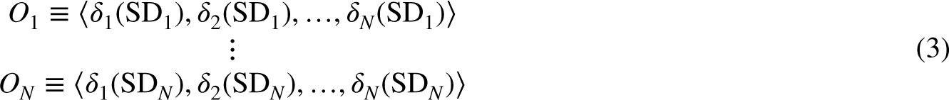
By applying this procedure to a set of $D$ original datasets, we can create a dataset of meta-features that collects the $δ$ -based representation of the $| D | \times N$ oracles generated (one oracle per dataset $D \in D$ and ML family $y \in 1, \dots, N$ ), along with the corresponding oracle family $y$ for each tuple. This dataset can be used as a training set for developing a meta-model to predict the family $y$ (the output) of any new black-box model. This prediction would be based on a set of $δ$ values representing the input attributes for the meta-model learning problem. In other words, given the $δ$ values obtained from a set of surrogate models, the meta-model can predict the family of black-box models. This meta-model represents a similar approach to the top meta-model in stacking ensembles [51], but in our case it is used specifically for ML family identification.

4. Evaluation

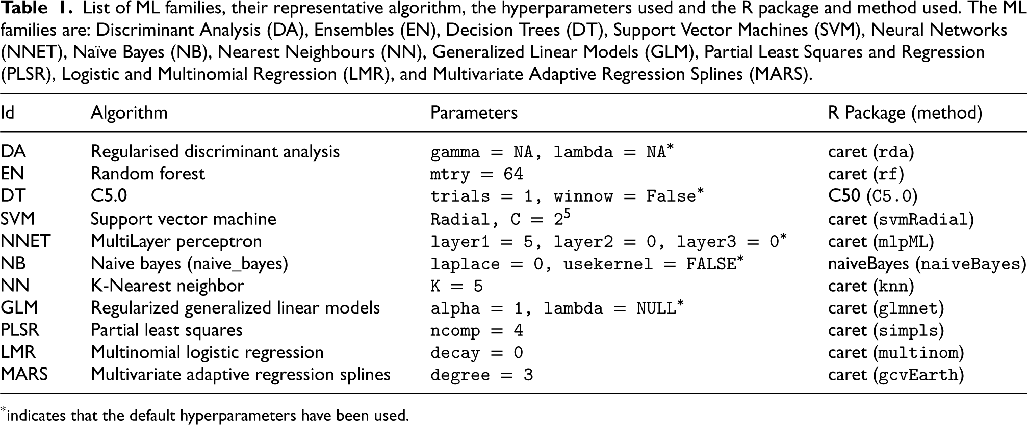
This section describes the experiments carried out to evaluate the proposed family identification methods (For the sake of reproducibility and replicability, all the experiments, code, data and plots can be found at https://github.com/rfabra/cracking_blackbox). All the experiments have been developed primarily in R [52] and, in particular, using the package Caret [53], to tune and train the different ML models.

Table 1
List of ML families, their representative algorithm, the hyperparameters used and the R package and method used. The ML families are: Discriminant Analysis (DA), Ensembles (EN), Decision Trees (DT), Support Vector Machines (SVM), Neural Networks (NNET), Naïve Bayes (NB), Nearest Neighbours (NN), Generalized Linear Models (GLM), Partial Least Squares and Regression (PLSR), Logistic and Multinomial Regression (LMR), and Multivariate Adaptive Regression Splines (MARS).

Id Algorithm Parameters R Package (method)

DA Regularised discriminant analysis gamma = NA, lambda = NA* caret (rda)

EN Random forest mtry = 64 caret (rf)

DT C5.0 trials = 1, winnow = False* C50 (C5.0)

SVM Support vector machine Radial, C = 2⁵ caret (svmRadial)

NNET MultiLayer perceptron layer1 = 5, layer2 = 0, layer3 = 0* caret (mlpML)

NB Naive bayes (naive_bayes) laplace = 0, usekernel = FALSE* naiveBayes (naiveBayes)

NN K-Nearest neighbor K = 5 caret (knn)

GLM Regularized generalized linear models alpha = 1, lambda = NULL* caret (glmnet)

PLSR Partial least squares ncomp = 4 caret (simpls)

LMR Multinomial logistic regression decay = 0 caret (multinom)

MARS Multivariate adaptive regression splines degree = 3 caret (gcvEarth)

*indicates that the default hyperparameters have been used.

Id	Algorithm	Parameters	R Package (method)
DA	Regularised discriminant analysis	gamma = NA, lambda = NA*	caret (rda)
EN	Random forest	mtry = 64	caret (rf)
DT	C5.0	trials = 1, winnow = False*	C50 (C5.0)
SVM	Support vector machine	Radial, C = 2⁵	caret (svmRadial)
NNET	MultiLayer perceptron	layer1 = 5, layer2 = 0, layer3 = 0*	caret (mlpML)
NB	Naive bayes (naive_bayes)	laplace = 0, usekernel = FALSE*	naiveBayes (naiveBayes)
NN	K-Nearest neighbor	K = 5	caret (knn)
GLM	Regularized generalized linear models	alpha = 1, lambda = NULL*	caret (glmnet)
PLSR	Partial least squares	ncomp = 4	caret (simpls)
LMR	Multinomial logistic regression	decay = 0	caret (multinom)
MARS	Multivariate adaptive regression splines	degree = 3	caret (gcvEarth)

Table 2

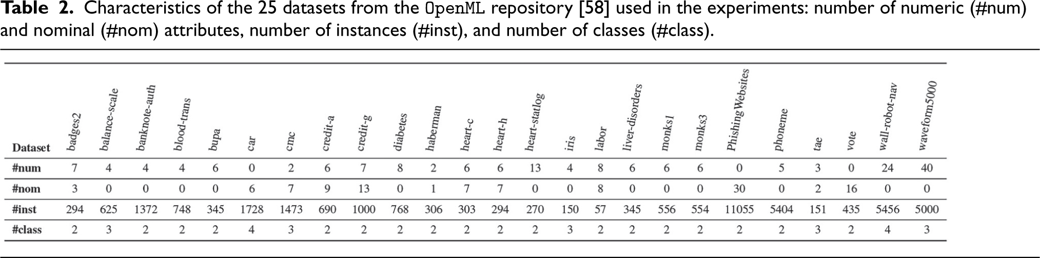
Characteristics of the 25 datasets from the OpenML repository [58] used in the experiments: number of numeric (#num) and nominal (#nom) attributes, number of instances (#inst), and number of classes (#class).

For the experiments, we have selected a set of machine learning techniques that are commonly used in practice and are typically grouped into families based on their formulation and learning strategy, as documented in [54, 55, 56, 57]. Specifically, we considered $N =$ 11 machine learning families, as listed in Table 1, and for each family $y \in N$ we selected only one of the algorithms from that family (Algorithm column in Table 1). To evaluate our meta-similarity approach, we needed a sufficiently large dataset of meta-features. For this purpose, we used a collection of 25 datasets from OpenML-CC18, a curated comprehensive classification benchmark from OpenML [58] (see Table 2). We applied a basic cleaning procedure to each dataset, which included removing missing values, constant attributes, and noise or duplicate examples. In addition, we performed two preprocessing steps, namely scaling and centering the data, to facilitate the learning of some models.

For each dataset, we trained $N$ models (oracles) belonging to the different families introduced in Table 1, thus learning $| D | \times N = 25 \times 11 = 275$ oracle models. For each of these oracles, we generated a surrogate dataset SD which we used to learn the surrogate models. Each instance of a SD is randomly generated following the uniform distribution: for each numerical feature, we randomly generated a number between its minimum and maximum values; for each discrete feature, we randomly selected one of the possible values it could take. Note that we need to generate an adequate number of examples for SD in order to identify the model family of $O$ with a reasonable degree of accuracy. In this regard, we have studied the effect that the size of SD can have on the accuracy of family identification (the results of this study are presented in the Appendix A) and, taking these results as a reference, we generate SD with a size equal to 100 multiplied by the number of features.

To evaluate each surrogate model $A_{i}$ , we generate another surrogate dataset (SD) of the same size, and then compare the outputs of the original oracle ( $O$ ) with those obtained from $A_{i}$ to obtain the different $δ_{i}$ values, as described above. These $δ_{i}$ values are then used to generate a dataset of meta-features that are used to train the meta-model in our meta-similarity approach. Specifically, we train and fine tune (see Appendix B) a Random Forest algorithm [59] on this dataset of meta-features, using the oracle’s ML family as class labels. To evaluate the performance of the meta-model, we use a leave-1-out cross-validation procedure, where in each fold, one dataset is used to test the meta-model and the remaining datasets are used to train it. Finally, note that given the novelty of our approach, direct comparisons with established methods are not feasible. Instead, we benchmark against a random selection baseline that randomly assigns ML families based on their distribution in our dataset.

Table 3

Confusion matrices (actual class in rows vs. predicted class in columns) showing the results for the Maximum Similarity approach evaluated for two different scenarios. The matrix on the top corresponds to the crisp scenario, where the $δ$ metric used is Cohen’s kappa coefficient ( $δ_{i} = κ_{i}$ ). The accuracy achieved in this scenario was 30.9%. The matrix on the bottom corresponds to the soft scenario, where the $δ$ metric is the L1 norm ( $δ_{i} = μ_{i}$ ). The accuracy achieved in this scenario was 30.6%.

Family	DA	EN	DT	SVM	NNET	NB	NN	GLM	PLSR	LMR	MARS	Total
DA	1	3	0	10	0	0	0	3	0	8	0	25
EN	0	12	3	5	1	0	1	0	0	0	3	25
DT	0	10	11	2	1	0	0	0	0	0	1	25
SVM	0	2	1	17	0	1	1	0	0	0	3	25
NNET	0	1	1	1	3	0	0	5	0	14	0	25
NB	1	3	0	11	0	0	0	4	0	2	4	25
NN	4	3	0	11	1	0	2	2	0	1	1	25
GLM	0	4	0	0	2	0	0	10	0	9	0	25
PLSR	0	2	1	1	1	0	0	8	0	12	0	25
LMR	0	1	0	2	3	0	0	3	0	16	0	25
MARS	0	6	3	4	0	0	0	0	0	0	12	25
Total	6	47	20	64	12	1	4	35	0	62	24	275
Family	DA	EN	DT	SVM	NNET	NB	NN	GLM	PLSR	LMR	MARS	Total
DA	9	2	0	6	0	2	0	4	0	0	2	25
EN	1	6	0	0	0	2	0	2	14	0	0	25
DT	0	8	9	2	2	1	0	0	3	0	0	25
SVM	0	6	0	3	0	0	1	0	14	0	1	25
NNET	3	4	0	0	9	0	0	1	8	0	0	25
NB	1	2	0	12	0	5	0	1	1	1	2	25
NN	3	7	0	5	0	2	1	1	4	0	2	25
GLM	5	5	0	1	0	3	0	5	6	0	0	25
PLSR	0	0	0	0	0	1	0	0	24	0	0	25
LMR	6	2	0	0	0	5	0	5	3	4	0	25
MARS	0	5	2	6	0	1	0	0	1	0	10	25
Total	28	47	11	35	11	22	2	19	78	5	17	275

4.1 Results of the maximum similarity approach

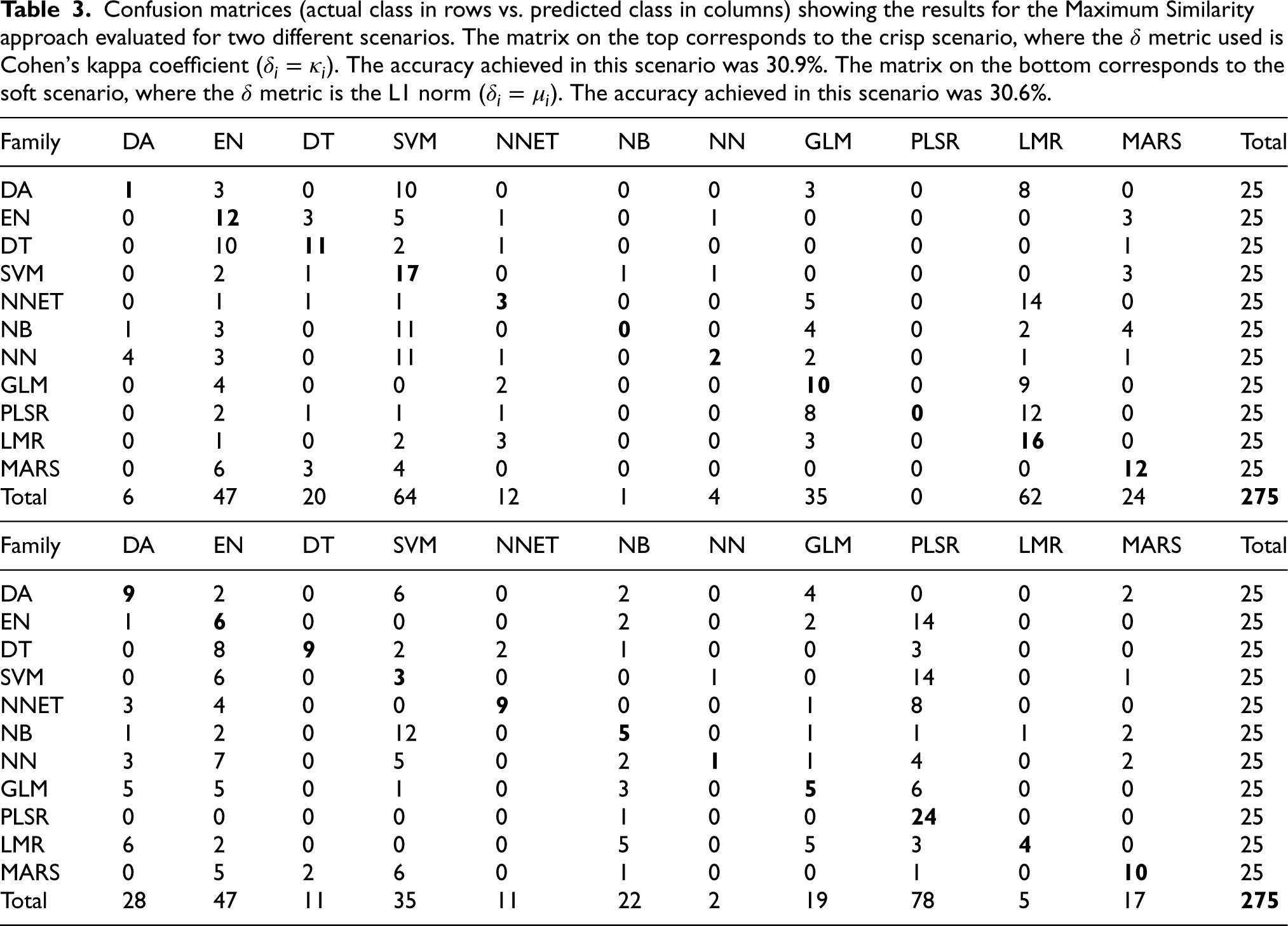
Table 3 shows the confusion matrices for the experiments using the Maximum Similarity approach. In the crisp scenario (as shown in the top matrix of Table 3), we observed that the SVM and LMR families had the highest number of positive identifications, with 17 (68%) and 16 (64%) correct identifications, respectively. The MARS and EN families followed closely with 12 correct identifications each (48% success rate). However, there were some families for which the maximum similarity approach performed very poorly, such as PLSR and NB, for which none of the models predicted correctly. In addition, the DA, NN and NNET families had only 1, 2 and 3 correct identifications, respectively. Most of these families were highly confused with SVM and LMR, and sometimes with GLM (mainly PLSR, NB, and NNET). We also noticed that GLM was often confused with LMR, with 9 incorrect identifications, and DT was confused with EN 10 times. Looking at the predicted family column, we observed that the models with the highest positive identifications (SVM, LMR, MARS, and EN) tended to be over-predicted, i.e. many of the other families were strongly confused with them. Conversely, the poorest performing families (PLSR, NB and NN) tended to be under-predicted, i.e. almost no correct or incorrect identifications were made for these families. In summary, the maximum similarity approach achieved an overall accuracy of 30.6% in the crisp scenario.

In the soft scenario (bottom matrix in Table 3), the PLSR family achieves the best results with 24 correct identifications (96%), followed by MARS with 10 correct identifications (40%). Other families such as NNET, DT and DA achieve similar results with 9 correct identifications each. However, PLSR tends to be over-predicted as many other families are often confused with it. The families with the fewest correct identifications are NN with only 1 correct identification, followed by SVM with 3 correct identifications, and LMR, NB and GLM with 4, 5 and 5 correct identifications respectively. NN is most often confused with EN with 7 incorrect identifications, but also with SVM with 5 incorrect identifications. The EN and SVM families are strongly confused with PLSR with 14 incorrect identifications. Similarly, the NNET family is often confused with PLSR with 8 false identifications. The LMR family tends to be confused with DA, NB and GLM. The GLM family is mainly confused with PLSR, DA and EN. In this scenario, the overall accuracy of the maximum similarity approach was 30.9%, almost identical to that obtained in the crisp scenario.

The results of our experiments suggest that the decision boundaries between machine learning families may not be clearly defined. Despite its limitations, our maximum similarity method significantly outperforms the results of a random baseline, which would predict an accuracy of around 9%. This superior performance highlights the effectiveness of the dissimilarity measures we use, allowing us to effectively extract and use relevant information from the model’s responses, thus providing an informed approach to model family identification. Interestingly, we obtained a very similar overall accuracy for both the crisp and soft scenarios, with values of 30.6% and 30.9% respectively. However, the families that were correctly identified in both scenarios were quite different, as can be seen from Table 3 (top and bottom). This suggests that, depending on the type of predictions provided (class labels vs. class conditional probabilities), some ML families may be easier to identify than others. Overall, our results suggest that the problem of identifying the model family of a black-box model is not trivial, but our maximum similarity approach is a promising starting point.

Table 4
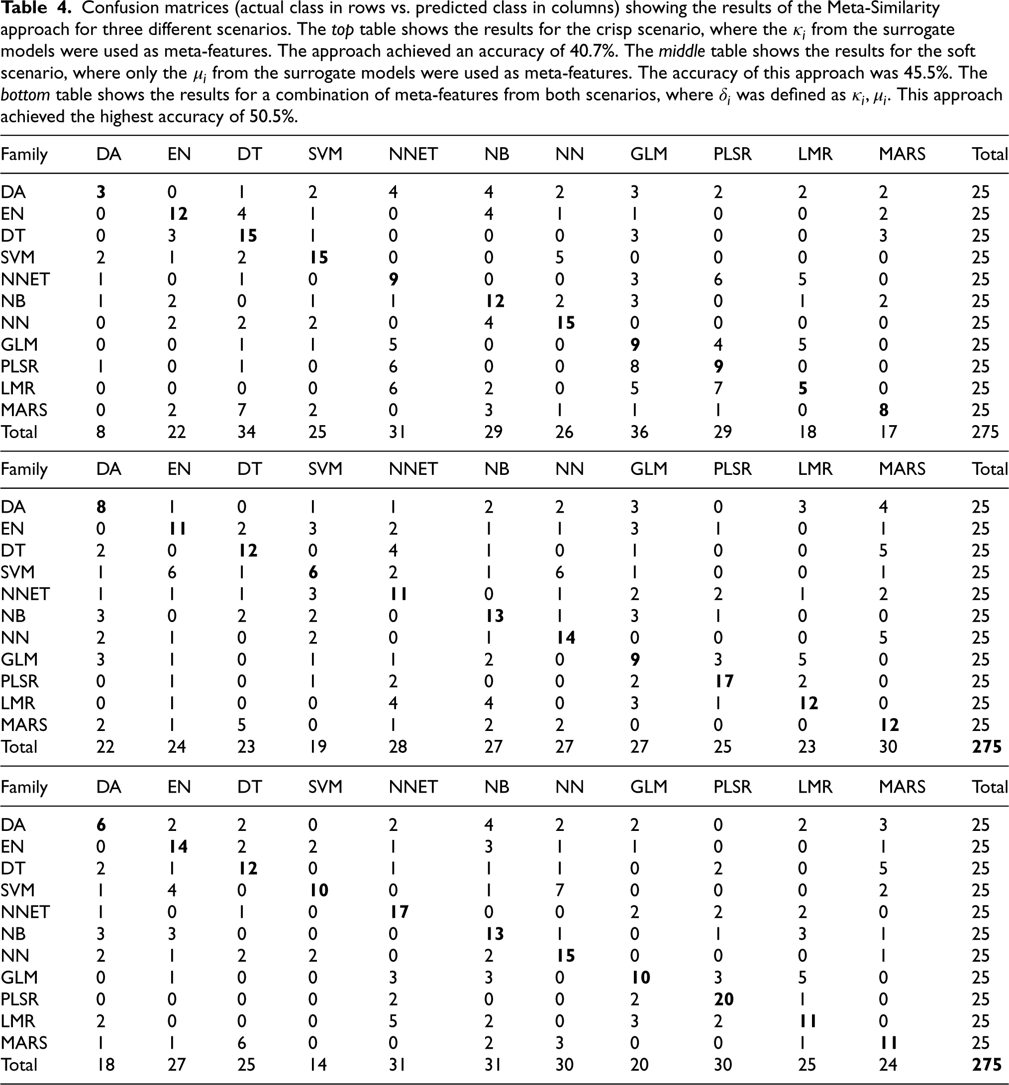
Confusion matrices (actual class in rows vs. predicted class in columns) showing the results of the Meta-Similarity approach for three different scenarios. The top table shows the results for the crisp scenario, where the $κ_{i}$ from the surrogate models were used as meta-features. The approach achieved an accuracy of 40.7%. The middle table shows the results for the soft scenario, where only the $μ_{i}$ from the surrogate models were used as meta-features. The accuracy of this approach was 45.5%. The bottom table shows the results for a combination of meta-features from both scenarios, where $δ_{i}$ was defined as $κ_{i}, μ_{i}$ . This approach achieved the highest accuracy of 50.5%.

Family DA EN DT SVM NNET NB NN GLM PLSR LMR MARS Total

DA 3 0 1 2 4 4 2 3 2 2 2 25

EN 0 12 4 1 0 4 1 1 0 0 2 25

DT 0 3 15 1 0 0 0 3 0 0 3 25

SVM 2 1 2 15 0 0 5 0 0 0 0 25

NNET 1 0 1 0 9 0 0 3 6 5 0 25

NB 1 2 0 1 1 12 2 3 0 1 2 25

NN 0 2 2 2 0 4 15 0 0 0 0 25

GLM 0 0 1 1 5 0 0 9 4 5 0 25

PLSR 1 0 1 0 6 0 0 8 9 0 0 25

LMR 0 0 0 0 6 2 0 5 7 5 0 25

MARS 0 2 7 2 0 3 1 1 1 0 8 25

Total 8 22 34 25 31 29 26 36 29 18 17 275

Family DA EN DT SVM NNET NB NN GLM PLSR LMR MARS Total

DA 8 1 0 1 1 2 2 3 0 3 4 25

EN 0 11 2 3 2 1 1 3 1 0 1 25

DT 2 0 12 0 4 1 0 1 0 0 5 25

SVM 1 6 1 6 2 1 6 1 0 0 1 25

NNET 1 1 1 3 11 0 1 2 2 1 2 25

NB 3 0 2 2 0 13 1 3 1 0 0 25

NN 2 1 0 2 0 1 14 0 0 0 5 25

GLM 3 1 0 1 1 2 0 9 3 5 0 25

PLSR 0 1 0 1 2 0 0 2 17 2 0 25

LMR 0 1 0 0 4 4 0 3 1 12 0 25

MARS 2 1 5 0 1 2 2 0 0 0 12 25

Total 22 24 23 19 28 27 27 27 25 23 30 275

Family DA EN DT SVM NNET NB NN GLM PLSR LMR MARS Total

DA 6 2 2 0 2 4 2 2 0 2 3 25

EN 0 14 2 2 1 3 1 1 0 0 1 25

DT 2 1 12 0 1 1 1 0 2 0 5 25

SVM 1 4 0 10 0 1 7 0 0 0 2 25

NNET 1 0 1 0 17 0 0 2 2 2 0 25

NB 3 3 0 0 0 13 1 0 1 3 1 25

NN 2 1 2 2 0 2 15 0 0 0 1 25

GLM 0 1 0 0 3 3 0 10 3 5 0 25

PLSR 0 0 0 0 2 0 0 2 20 1 0 25

LMR 2 0 0 0 5 2 0 3 2 11 0 25

MARS 1 1 6 0 0 2 3 0 0 1 11 25

Total 18 27 25 14 31 31 30 20 30 25 24 275

Family	DA	EN	DT	SVM	NNET	NB	NN	GLM	PLSR	LMR	MARS	Total
DA	3	0	1	2	4	4	2	3	2	2	2	25
EN	0	12	4	1	0	4	1	1	0	0	2	25
DT	0	3	15	1	0	0	0	3	0	0	3	25
SVM	2	1	2	15	0	0	5	0	0	0	0	25
NNET	1	0	1	0	9	0	0	3	6	5	0	25
NB	1	2	0	1	1	12	2	3	0	1	2	25
NN	0	2	2	2	0	4	15	0	0	0	0	25
GLM	0	0	1	1	5	0	0	9	4	5	0	25
PLSR	1	0	1	0	6	0	0	8	9	0	0	25
LMR	0	0	0	0	6	2	0	5	7	5	0	25
MARS	0	2	7	2	0	3	1	1	1	0	8	25
Total	8	22	34	25	31	29	26	36	29	18	17	275

Family	DA	EN	DT	SVM	NNET	NB	NN	GLM	PLSR	LMR	MARS	Total
DA	8	1	0	1	1	2	2	3	0	3	4	25
EN	0	11	2	3	2	1	1	3	1	0	1	25
DT	2	0	12	0	4	1	0	1	0	0	5	25
SVM	1	6	1	6	2	1	6	1	0	0	1	25
NNET	1	1	1	3	11	0	1	2	2	1	2	25
NB	3	0	2	2	0	13	1	3	1	0	0	25
NN	2	1	0	2	0	1	14	0	0	0	5	25
GLM	3	1	0	1	1	2	0	9	3	5	0	25
PLSR	0	1	0	1	2	0	0	2	17	2	0	25
LMR	0	1	0	0	4	4	0	3	1	12	0	25
MARS	2	1	5	0	1	2	2	0	0	0	12	25
Total	22	24	23	19	28	27	27	27	25	23	30	275

Family	DA	EN	DT	SVM	NNET	NB	NN	GLM	PLSR	LMR	MARS	Total
DA	6	2	2	0	2	4	2	2	0	2	3	25
EN	0	14	2	2	1	3	1	1	0	0	1	25
DT	2	1	12	0	1	1	1	0	2	0	5	25
SVM	1	4	0	10	0	1	7	0	0	0	2	25
NNET	1	0	1	0	17	0	0	2	2	2	0	25
NB	3	3	0	0	0	13	1	0	1	3	1	25
NN	2	1	2	2	0	2	15	0	0	0	1	25
GLM	0	1	0	0	3	3	0	10	3	5	0	25
PLSR	0	0	0	0	2	0	0	2	20	1	0	25
LMR	2	0	0	0	5	2	0	3	2	11	0	25
MARS	1	1	6	0	0	2	3	0	0	1	11	25
Total	18	27	25	14	31	31	30	20	30	25	24	275

4.2 Results of the meta-similarity approach

The confusion matrix for the meta-similarity approach in the crisp scenario is shown in Table 4 on the top. The results show an improvement over the maximum similarity approach, with an overall accuracy of 40.7% (compared to 30.6% obtained by the maximum similarity approach in the crisp scenario). We can see that SVM, DT and NN are now the easiest family to identify, with 15 correct identifications (60%), followed by EN and NB with 12 correct identifications (48%). On the other hand, DA and LMR families were the most difficult to identify, with 3 and 5 correct identifications, respectively. In terms of confusion patterns, SVM is confused mainly with NN and sometimes with DA, DT and EN. DT is confused with EN, GLM and MARS. The NN family is confused with NB principally, but also with EN, DT and SVM. DA is frequently misclassified as NNET and NB, but also with other models. The LMR model is mainly confused with PLSR, NNET and GLM, while GLM is often confused with LMR, NNET and PLSR. PLSR is mainly confused with GLM, and NNET. In addition, MARS is confused with DT. Overall, we can see that some families have significantly improved results compared to the maximum similarity approach, such as NN, NB, PLSR and NNET. However, the LMR and MARS families present worse results in the meta-similarity approach. SVM and GLM families have slightly worse results in the meta-similarity approach.

The Table 4 on the middle shows the results of the meta-similarity approach for the soft scenario. Using the meta-features based on the $μ$ measure, the approach achieves a global accuracy of 45.5%, slightly higher than the value obtained in the crisp scenario. We observe that PLSR and NN are the easiest families to identify, with 17 (68%) and 14 (56%) correct identifications, respectively. Those families that seem to be the most difficult to identify are SVM, DA and GLM, with only 6 (24%), 8 (32%), and 9 (36%) correct identifications, respectively . DA is mainly confused with MARS, LMR and GLM, while GLM is often confused with LMR and PLSR and DA (between 3–5 times). SVM is often confused with NN and EN. Comparing the results of the meta-similarity approach for the soft scenario with those obtained with the maximum similarity approach in the same scenario, we see that PLSR is the only family for which the results are significantly worse, going from 24 correct identifications to 17. The DA family obtains slightly worse results, going from 9 correct identifications to 8. NN, NB, LMR and EN are the families for which the results improve the most (especially NN, going from 1 to 14 correct identifications). The number of successful identifications remains more or less the same for the other families, with slight improvements for GLM, DT, SVM, NNET, MARS.

In line with the results obtained using the maximum similarity approach, the meta-similarity approach shows that the effectiveness of ML family identification is largely influenced by the metric used for evaluation. This suggests that a hybrid approach that integrates the information from both similarity measures, $κ$ and $μ$ , could potentially outperform the individual approaches for family identification. Therefore, we conducted further experiments to evaluate the performance of a hybrid variant of the meta-similarity approach that combines $κ_{i}$ and $μ_{i}$ as meta-features. The results of this hybrid approach are presented in Table 4 (bottom).

As expected, we observed that the overall accuracy of the hybrid approach is the best of all the proposed approaches, achieving an accuracy of 50.5%. This approach also shows similar or improved identification results for most of the families compared to the previous meta-similarity approaches. For example, the EN, NNET, NB, NN and GLM families show 14, 17, 13, 15 and 10 correct identifications respectively, which is an improvement compared to the results obtained by the previous approaches. The SVM and LMR families obtain better results in the crisp scenario with the maximum-similarity approach (17 and 16, respectively). The identification of other families remains unchanged or slightly lower than the best result, such as DT, PLSR and MARS. However, DA emerges as the most difficult family to identify, with only 6 correct identifications. In addition, all the approaches provide poorer results in regard to the identification of this family.

The overall results of our experiments suggest that identifying the ML families of black-box models is a challenging but promising approach. The use of dissimilarity measures based on predicted class labels or class conditional probabilities has proven to be effective in identifying ML families with a reasonable degree of accuracy. It is important to note that the complexity of the family identification problem is due to the fact that many ML families share similar characteristics and decision boundaries. Therefore, it is difficult to find clear differences between them that allow for straightforward identification. This complexity is also reflected in the fact that the best performing approach varies depending on the evaluation metric used (i.e. $κ$ or $μ$ ). Despite these challenges, our results show that the meta-similarity approach outperforms the maximum similarity approach in terms of accuracy. However, this approach also presents a potential danger, as it could be used by malicious actors for adversarial attacks targeting a specific family.

5. Conclusions and future work

This work addresses the problem of identifying the model family of a black-box learning model. For this purpose, we propose two approaches based on dissimilarity measures $δ$ . The first approach, which we call the maximum similarity approach, uses Cohen’s kappa coefficient as $δ$ when the models are able to predict class labels (i.e. the crisp scenario). In this approach, several surrogate models from different learning families are trained on a set of artificial examples labelled by the black-box model (which acts as an oracle). The predicted machine learning family for the black box model is the one with the surrogate model that has the best value for $δ$ . The second approach, which we call the meta-similarity approach, uses the L1 norm as $δ$ for cases where the models predict class conditional probabilities (i.e. the soft scenario). This approach uses the $δ$ values as meta-features to represent the black-box model. These values are then used as metadata to learn a meta-model that can predict the learning family of a black-box model.

The experiments conducted in this study show that the first proposed approach for identifying ML families, based on $δ$ measures, performed poorly but was still able to improve the accuracy of the results over a random baseline. In contrast, the second approach, based on meta-models using abstract meta-features derived from dissimilarity measures, achieved significantly higher accuracy in identifying the ML families of black-box models. These results highlight the potential of using meta-models trained on abstract meta-features for ML family identification. This potential is further supported by the results obtained by combining the meta-features generated using both evaluation metrics, which yielded the highest overall accuracy among the proposed approaches.

To enhance the performance of our meta-model-based approach for identifying the family of black-box learning models, we plan to investigate the use of additional measures of model divergence and diversity as meta-features. For example, measures such as Bhattacharyya distance [60], Jaccard similarity coefficient [61] and Tanimoto distance [62] have been proposed in the literature to compare probability density functions [63] and could be explored to capture different aspects of model dissimilarity. In addition to our focus on operational efficiency and effectiveness, we are also interested in exploring alternative query strategies for generating surrogate datasets. For example, Latin Hypercube [64], Centroidal Voronoi Tessellation [65] and Sobol [66] sampling approaches are promising alternatives that could improve the representativeness of surrogate datasets and increase the accuracy of the model identification process.

Footnotes

Acknowledgments

This work has been partially supported by the grant CIPROM/2022/6 funded by Generalitat Valenciana, the MIT-Spain – INDITEX Sustainability Seed Fund under project COST-OMIZE, the grant PID2021-122830OB-C42 funded by MCIN/AEI/10.13039/501100011033 and ERDF A way of making Europe, EU’s Horizon 2020 research and innovation programme under grant agreement No. 952215 (TAILOR).

Appendix A. Study of the impact of the surrogate dataset size

Generating the surrogate dataset SD is a crucial step in identifying the model family, and our approach for generating SD follows a simple strategy of employing a uniform distribution for each feature. This is because we treat the oracle as a black-box model, meaning that we have no knowledge of the training data it used. Therefore, we cannot use any information from the training data, such as data sparsity, separability, or attribute correlations, to guide the generation of the surrogate dataset.

The size of the surrogate dataset is thus a decisive aspect of our methodology, as it is the basis for learning and evaluating the surrogate models. In this sense, we conducted an illustrative experimental study to observe how the size of the dataset affects the accuracy of the family identification task. The method we followed is similar to that described in Section 3.1, where we generate oracles and their corresponding surrogate models, but we varied the size of the surrogate dataset. Specifically, we computed the size of the surrogate dataset as | SD | = θ × F , where F is the number of attributes in the problem and θ is a size factor that we manually set to 10, 100 and 1000 to consider different orders of magnitude. To identify the model family of an oracle, we used the maximum similarity approach in a crisp scenario for efficiency reasons. We compared the results of the oracles and the surrogate models using the κ metric, as described in Section 3.3. To obtain more significant results, we repeated the entire procedure 10 times for each surrogate dataset size and dataset, and averaged the results.

To evaluate the impact of the size factor ( θ ) of the surrogate dataset on the family identification performance, we conducted an illustrative experiment on ten OpenML datasets. The results are summarised in Appendix Figure A.1. We can see that for three of the datasets (badges, car and scale) the highest accuracy is achieved with a size factor of 100. On the other hand, for four datasets (diabetes, credit-a, credit-g, and banknote authentication), the performance gain decreases significantly beyond a size factor of 100, compared to the jump between size factors of 10 and 100. It is worth noting that using a small number of examples ( θ ⩽ 100) does not give very accurate results for family identification. Similarly, using a large number of examples ( ⩾ 300) does not necessarily improve identification performance (see the average curve in Appendix Figure A1). Therefore, finding an optimal size factor for the surrogate dataset is crucial for achieving good performance in family identification. Further research could investigate the possibility of determining this optimal size factor in a more automated way, based on the properties of the dataset and the black box model.

It might seem that a larger SD would provide more information, leading to better accuracy in model family identification. However, in our simple experiment we observed that the maximum accuracy for family identification was achieved when using a θ between 100 and 1000. Increasing the size factor by an order of magnitude (up to a θ of 1000) did not improve the accuracy of model family identification. This phenomenon may occur because the better the surrogate models mimic the decision boundaries, the more detailed (and similar) the decision boundaries of the surrogate models become, and the less distinguishable they become. These results suggest that some appropriate values for θ would be around 100. So for the rest of the experiments in this paper, we chose a value of θ = 100 when generating the surrogate datasets.

Appendix B. Exploration of the Meta-model hyperparameters

Our meta-model, a Random Forest algorithm [59], gives us the opportunity to tune its hyper-parameters. This allows us to delve deeper into the task of identifying model families and the different representations for each scenario. By performing a grid search and cross-validation to find the best hyperparameters, first, we adjusted the number of trees in the meta-model (NT), ranging from 1 to 1024. This variation helped us to assess the complexity inherent in the datasets of meta-features created using κ , μ or a combination of both. Essentially, the number of trees required reflects the complexity of the patterns in the dataset – more trees indicate more complex patterns. The results of this analysis are summarised in Appendix Table B1. We also changed the number of features (NF) to be considered in each split, which affected the optimisation of the model. The results, detailed in Appendix Table B2, highlight the configurations that achieved the highest accuracy, which we then applied in subsequent experiments detailed in Section 4.2.

The variations in these two parameters highlight interesting aspects of the identification of model families using a meta-similarity approach. In the crisp scenario, optimal performance was achieved with 64 trees, indicating that additional trees up to 1024 do not significantly improve the accuracy of the meta-model. This implies that the meta-features in the crisp scenario provide a simple representation, achieving an accuracy of 40.7% with these features alone. For the soft scenario, at least 128 trees were required to achieve maximum accuracy, suggesting a more complex set of features. Combining both meta-features required 256 trees for maximum accuracy.

Looking at the ’number of features’ parameter, it is clear that not all available features were used to achieve maximum accuracy in all scenarios; 7 out of 11 features for the crisp scenario, 10 out of 11 for the soft scenario, and 18 out of 22 for the hybrid scenario. This suggests the presence of redundant meta-features, probably generated by closely related model families. This is shown in more detail in Appendix Figure B1: the most relevant features used in the hybrid approach are also the most used within their individual methods. Interestingly, both the hybrid and crisp methods exclude the same meta-features related to kappa values for classifiers such as DA, MLP, NB and PLSR. The soft method, on the other hand, only excludes SVM. Decision trees (DT) and generalised linear models (GLM) emerge as significant in all three methods. While NB, PLSR and DA are considered less significant in the crisp method, it is noteworthy that they are in the top five in both the soft and hybrid approaches. However, neural networks (NNET) and SVM consistently show low relevance, either not being selected at all or being selected last, indicating their limited utility in family identification tasks.

Overall, the meta-features of the crisp scenario, which require fewer trees for optimal performance, show simpler patterns. In contrast, the meta-features of the hybrid approach, which require more trees for peak accuracy, offer a more complex representation. Simpler representations require fewer features for higher accuracy.

References

Fabra-Boluda

Ferri

Hernández-Orallo

Martínez-Plumed

Ramírez-Quintana

M.J.

, Modelling Machine Learning Models, in: 3rd Conf. on” Philosophy and Theory of Artificial Intelligence, Springer, (2017), 175–186.

Joseph

A.D.

Nelson

Rubinstein

B.I.

Tygar

, Adversarial machine learning, Cambridge University Press, (2018).

Vorobeychik

Kantarcioglu

Brachman

Stone

Rossi

, Adversarial machine learning, 12, Springer, (2018).

Molnar

et al, Interpretable machine learning: A guide for making black box models explainable, Christoph Molnar, Leanpub (2018).

Hassija

Chamola

Mahapatra

Singal

Goel

Huang

Scardapane

Spinelli

Mahmud

Hussain

, Interpreting black-box models: a review on explainable artificial intelligence, Cognitive Computation (2023), 1–30.

Biggio

Corona

Nelson

Rubinstein

B.I.

Maiorca

Fumera

Giacinto

Roli

, Security evaluation of support vector machines in adversarial environments, in: Support Vector Machines Applications, Springer, (2014), 105–153.

Wang

Sun

Yuan

Hossain

Poor

H.V.

, Adversarial attacks and defenses in machine learning-powered networks: a contemporary survey, arXiv preprint arXiv:2303.06302. (2023).

Huang

Joseph

A.D.

Nelson

Rubinstein

B.I.

Tygar

, Adversarial machine learning, in: Proc. of the 4th ACM WS. on Security and artificial intelligence, (2011), 43–58.

Tramèr

Zhang

Juels

Reiter

M.K.

Ristenpart

, Stealing machine learning models via prediction APIs., in: USENIX Security Symp., (2016), 601–618.

10.

Papernot

McDaniel

Goodfellow

, Transferability in machine learning: from phenomena to black-box attacks using adversarial samples, arXiv preprint arXiv:1605.07277. (2016).

11.

Lee

Shin

, A simple unified framework for detecting out-of-distribution samples and adversarial attacks, Advances in Neural Information Processing Systems 31 (2018).

12.

Geng

Huang

S.-J.

Chen

, Recent advances in open set recognition: A survey, IEEE Transactions on Pattern Analysis and Machine Intelligence 43(10) (2020), 3614–3631.

13.

Kwon

Prabhushankar

Temel

AlRegib

, Novelty detection through model-based characterization of neural networks, in: 2020 IEEE International Conference on Image Processing (ICIP), IEEE, (2020), 3179–3183.

14.

Boukerche

Zheng

Alfandi

, Outlier detection: Methods, models, and classification, ACM Computing Surveys (CSUR) 53(3) (2020), 1–37.

15.

Nassif

A.B.

Talib

M.A.

Nasir

Dakalbab

F.M.

, Machine learning for anomaly detection: A systematic review, Ieee Access 9 (2021), 78658–78700.

16.

Jobin

Ienca

Vayena

, The global landscape of AI ethics guidelines, Nature Machine Intelligence 1(9) (2019), 389–399.

17.

Gneiting

Raftery

A.E.

, Weather forecasting with ensemble methods, Science 310(5746) (2005), 248–249.

18.

Kirkwood

Economou

Odbert

Pugeault

, A framework for probabilistic weather forecast post-processing across models and lead times using machine learning, Philosophical Transactions of the Royal Society A 379(2194) (2021), 20200099.

19.

Štrumbelj

, On determining probability forecasts from betting odds, International Journal of Forecasting 30(4) (2014), 934–943.

20.

Stübinger

Mangold

Knoll

, Machine learning in football betting: Prediction of match results based on player characteristics, Applied Sciences 10(1) (2019), 46.

21.

Tausczik

Y.R.

Pennebaker

J.W.

, The Psychological Meaning of Words: LIWC and Computerized Text Analysis Methods, Journal of Language and Social Psychology 29(1) (2010), 24–54.

22.

Kumar

Srinivasan

Cheng

W.-H.

Zomaya

A.Y.

, Hybrid context enriched deep learning model for fine-grained sentiment analysis in textual and visual semiotic modality social data, Information Processing and Management 57(1) (2020), 102141.

23.

Kearns

, Efficient noise-tolerant learning from statistical queries, Journal of the ACM (JACM) 45(6) (1998), 983–1006.

24.

Valiant

L.G.

, A theory of the learnable, Communications of the ACM 27(11) (1984), 1134–1142.

25.

Angluin

, Learning regular sets from queries and counterexamples, Information and Computation 75(2) (1987), 87–106.

26.

Angluin

, Queries and concept learning, Machine Learning 2(4) (1988), 319–342.

27.

Benedek

G.M.

Itai

, Learnability with respect to fixed distributions, Theoretical Computer Science 86(2) (1991), 377–389.

28.

Ren

Xiao

Chang

Huang

P.-Y.

Gupta

B.B.

Chen

Wang

, A survey of deep active learning, ACM Computing Surveys (CSUR) 54(9) (2021), 1–40.

29.

Settles

, From theories to queries: Active learning in practice, in: Active Learning and Experimental Design WS. in conjunction with AISTATS 2010, (2011), 1–18.

30.

Wiyatno

R.R.

Dia

De Berker

, Adversarial Examples in Modern Machine Learning: A Review , arXiv preprint arXiv:1911.05268. (2019).

31.

Tabassi

Burns

K.J.

Hadjimichael

Molina-Markham

A.D.

Sexton

J.T.

, A taxonomy and terminology of adversarial machine learning, NIST IR2019 (2019), 1–29.

32.

Zhu

Yang

Cao

Chen

, Security matters: A survey on adversarial machine learning, arXiv preprint arXiv:1810.07339. (2018).

33.

Biggio

Roli

, Wild patterns: Ten years after the rise of adversarial machine learning, in: Proc. of the 2018 ACM SIGSAC Conf. on Computer and Communications Security (2018), 2154–2156.

34.

Ilyas

Engstrom

Athalye

Lin

, Black-box adversarial attacks with limited queries and information, in: International Conf. on Machine Learning, PMLR, (2018), 2137–2146.

35.

Papernot

McDaniel

Jha

Fredrikson

Celik

Z.B.

Swami

, The limitations of deep learning in adversarial settings, in: Security and Privacy (EuroS&P), 2016 IEEE European Symposium on, IEEE, (2016), 372–387.

36.

Papernot

McDaniel

Jha

Swami

, Distillation as a defense to adversarial perturbations against deep neural networks, in: Security and Privacy (SP), 2016 IEEE Symposium on, IEEE, (2016), 582–597.

37.

Papernot

McDaniel

Goodfellow

Jha

Celik

Z.B.

Swami

, Practical black-box attacks against machine learning, in: Proc. of the 2017 ACM on Asia Conf. on Computer And Communications Security, (2017), 506–519.

38.

Yuan

Zhu

, Adversarial examples: Attacks and defenses for deep learning, IEEE Transactions on Neural Networks and Learning Systems 30(9) (2019), 2805–2824.

39.

Domingos

, Knowledge discovery via multiple models, Intelligent Data Analysis 2(3) (1998), 187–202.

40.

Blanco-Vega

Hernández-Orallo

Ramírez-Quintana

, Analysing the trade-off between comprehensibility and accuracy in mimetic models, in: Discovery Science, (2004), 35–39.

41.

Wallace

C.S.

Boulton

D.M.

, An information measure for classification, The Computer Journal 11(2) (1968), 185–194.

42.

Yang

Jiang

Huang

Zhao

, Learning black-box attackers with transferable priors and query feedback, Advances in Neural Information Processing Systems 33 (2020), 12288–12299.

43.

Gunning

Stefik

Choi

Miller

Stumpf

Yang

G.-Z.

, XAI – Explainable artificial intelligence, Science robotics 4(37) (2019), eaay7120.

44.

Ribeiro

M.T.

Singh

Guestrin

, “Why should i trust you?”: Explaining the predictions of any classifier, in: Proc. of the 22Nd ACM SIGKDD International Conf. on Knowledge Discovery and Data Mining, KDD ’16, ACM, (2016), 1135–1144. ISBN 978-1-4503-4232-2. doi: https://doi.org/10.1145/2939672.2939778.

45.

Guidotti

Monreale

Ruggieri

Pedreschi

Turini

Giannotti

, Local rule-based explanations of black box decision systems, arXiv preprint arXiv:1805.10820. (2018).

46.

Maaroof

Moreno

Valls

Jabreel

Romero-Aroca

, Multi-Class Fuzzy-LORE: A Method for Extracting Local and Counterfactual Explanations Using Fuzzy Decision Trees, Electronics 12(10) (2023), 2215.

47.

S.J.

Schiele

Fritz

, Towards reverse-engineering black-box neural networks, Explainable AI: Interpreting, Explaining and Visualizing Deep Learning (2019), 121–144.

48.

Perkins

Adler-Golden

S.M.

Matthew

M.W.

Berk

Bernstein

L.S.

Lee

Fox

, Speed and accuracy improvements in FLAASH atmospheric correction of hyperspectral imagery, Optical Engineering 51(11) (2012), 111707.

49.

Landis

J.R.

Koch

G.G.

, An application of hierarchical kappa-type statistics in the assessment of majority agreement among multiple observers, Biometrics (1977), 363–374.

50.

Ferri

Hernández-Orallo

Modroiu

, An experimental comparison of performance measures for classification, Pattern Recognition Letters 30(1) (2009), 27–38.

51.

Wolpert

D.H.

, Stacked generalization, Neural Networks 5(2) (1992), 241–259.

52.

R Core Team, R: A Language and Environment for Statistical Computing, R Foundation for Statistical Computing, Vienna, Austria, (2019. http://www.R-project.org/.

53.

Kuhn

, Building Predictive Models in R Using the caret Package, Journal of Statistical Software, Articles 28(5) (2008), 1–26. doi: https://doi.org/10.18637/jss.v028.i05. https://www.jstatsoft.org/v028/i05.

54.

Duin

R.P.

Loog

Pȩkalska

Tax

D.M.

, Feature-based dissimilarity space classification, in: Recognizing Patterns in Signals, Speech, Images and Videos, Springer, (2010), 46–55.

55.

Fernández-Delgado

Cernadas

Barro

Amorim

, Do we need hundreds of classifiers to solve real world classification problems, J Mach Learn Res 15(1) (2014), 3133–3181.

56.

Martınez-Plumed

Prudêncio

R.B.

Martınez-Usó

Hernández-Orallo

, Making sense of item response theory in machine learning, in: Proc. of 22nd European Conf. on Artificial Intelligence (ECAI), Frontiers in Artificial Intelligence and Applications 285 (2016), 1140–1148.

57.

Smith

M.R.

Martinez

Giraud-Carrier

, An instance level analysis of data complexity, Machine Learning 95(2) (2014), 225–256.

58.

Vanschoren

Van Rijn

J.N.

Bischl

Torgo

, OpenML: networked science in machine learning, ACM SIGKDD Explorations Newsletter 15(2) (2014), 49–60.

59.

Breiman

, Random forests, Machine Learning 45(1) (2001), 5–32.

60.

Bhattacharyya

, On a measure of divergence between two statistical populations defined by their probability distribution, Bulletin of the Calcutta Mathematical Society 35 (1943), 99–110.

61.

Paul

et al, The distribution of the flora in the alpine zone. 1, New Phytologist 11(2) (1912), 37–50.

62.

Tanimoto

T.T.

, Elementary mathematical theory of classification and prediction, (1958).

63.

Cha

S.-H.

, Comprehensive survey on distance/similarity measures between probability density functions, City 1(2) (2007), 1.

64.

McKay

M.D.

Beckman

R.J.

Conover

W.J.

, Comparison of three methods for selecting values of input variables in the analysis of output from a computer code, Technometrics 21(2) (1979), 239–245.

65.

Gunzburger

, Advances in studies and applications of centroidal Voronoi tessellations, Numerical Mathematics: Theory, Methods and Applications 3(2) (2010), 119–142.

66.

Sobol’

I.M.

, On the distribution of points in a cube and the approximate evaluation of integrals, Zhurnal Vychislitel’noi Matematiki i Matematicheskoi Fiziki 7(4) (1967), 784–802.

Cracking black-box models: Revealing hidden machine learning techniques behind their predictions

Abstract

Keywords

1. Introduction

3. Model family identification

3.1 Generating surrogate models

3.3.1 Crisp classifiers

5. Conclusions and future work

Footnotes

Acknowledgments

Appendix A. Study of the impact of the surrogate dataset size

Appendix B. Exploration of the Meta-model hyperparameters

References