Sage Journals: Discover world-class research

Abstract

Knowledge graph embedding (KGE) is typically used for link prediction to automatically predict missing links in knowledge graphs. Current KGE models are mainly based on complicated mathematical associations, which are highly expressive but ignore the uniformity behind the classical bilinear translational model TransE, a model that embeds all entities of knowledge graphs in a uniform space, enabling accurate embeddings. This study analyses the uniformity of TransE and proposes a novel KGE model called ConvUs that follows uniformity with expressiveness. Based on the convolution neural network (CNN), ConvUs proposes constraints on convolution filter values and employs a multi-layer, multi-scale CNN architecture with a non-parametric L2 norm-based scoring function for the calculation of triple scores. This addresses potential uniformity-related issues in existing CNN-based KGE models, allowing ConvUs to maintain a uniform embedding space while benefiting from the powerful expressiveness of CNNs. Furthermore, circular convolution is applied to alleviate the potential orderliness contradictions, making ConvUs more suitable for conducting uniform space KGE. Our model outperformed the base model ConvKB and several baselines on the link prediction benchmark WN18RR and FB15k-237, demonstrating strong applicability and generalization and indicating that the uniformity of embedding space with high expressiveness enables more efficient knowledge graph embeddings.

Keywords

Knowledge graph embedding link prediction representation learning convolutional neural network

1. Introduction

A knowledge graph represents the knowledge of the objective world as a directed multi-relational graph in which the nodes and edges refer to entities and relations, respectively. A pair of nodes and the edge between them form a link corresponding to a knowledge triple, that is, $<$ head entity, relation, tail entity $>$ , as the basic unit of a knowledge graph. Knowledge graph has gained significant attention from academia and industry and has been used in various real-world applications such as Q&A [1], recommendation systems [2], image-text matching [3], etc. However, the current knowledge graphs suffer from incompleteness due to the inadequacy of raw data and knowledge graph-constructing techniques. Hence, link prediction is used to supplement the missing knowledge triples in existing knowledge graphs by inferring the potential combination of head entities, relations, and tail entities (that is, the unseen triples).

Common link prediction methods are based on the representation learning of knowledge graphs, namely knowledge graph embedding (KGE). Generally speaking, the existing methods represent entities and relations in a certain knowledge graph as implicit low-dimensional embeddings and use an overall scoring function to calculate the plausibility of each triple with its embeddings. The process of discovering potential triples with high plausibility is essentially link prediction. The core of KGE models typically lies in the way they score the triple: we refer to this process as the overall scoring function or score calculation of a certain model, which is trained with the embeddings to get more accurate triple scores. Existing KGE models for link prediction either use a traditional linear (bilinear) [4, 5, 6, 7, 8] or neural network-based nonlinear [9, 10, 11, 12, 13, 14] overall scoring function. In this paper, our basic idea is to incorporate the uniformity of the classical linear model TransE [4] with expressive nonlinear convolutional overall scoring function.

TransE is a typical example of a linear KGE model, whose basic idea is to consider the association between the embeddings of the head entities, tail entities, and relations as the translational relationship ${\bm{v}}_{h}+{\bm{v}}_{r}-{\bm{v}}_{t}=0$ ( ${\bm{v}}_{h},{\bm{v}}_{r},{\bm{v}}_{t}\in\mathbb{R}^{k}$ refer to the head entity, relation and tail entity embeddings). TransE is superior owing to its simplicity and clarity. It models all entities in a uniform space in which the associations between the head and tail entities are represented by a geometric relationship, making it reasonable and comprehensible. This uniformity of the embedding space provided by TransE improves one-to-one correspondence between the entities of the knowledge graph and embeddings, which is in line with the nature of knowledge graph representation learning and is essential for link prediction.

The problem of TransE lies in its expressiveness [7]. Other KGE models represent the relationship between the head and tail entity embeddings using projection or even more complicated nonlinear mathematical associations, which are more expressive than TransE but do not consider the uniformity of the entity embedding space. Among them, the CNN-based model ConvKB [9] introduces the idea of TransE into a CNN, it places restrictions on the length of the convolution filters and models only interactions between the dimensions of different embeddings (namely the heterogeneous interactions), a characteristic makes it similar to TransE and conform to uniformity to some extent. However, based on the definition of uniformity, the transformations of head and tail entity embeddings in each dimension should be completely identical. This suggests that the convolution filters of ConvKB should be constrained in their values to ensure a higher degree of uniformity. Moreover, after the convolutions, ConvKB adopts a fully connected layer to compute the triple plausibility scores. This process undoubtedly introduces numerous interactions between the embedding dimensions of multiple positions (i.e. the homogeneous interactions), which contradicts the inherent philosophy of the former convolutional layer in ConvKB and uniformity in particular.

To address the two issues with ConvKB and bring uniformity to expressive CNNs more comprehensively, we propose ConvUS – an improved CNN-based KGE model. Following the basic paradigm from ConvKB, this model first convolves the stacked triple embeddings and grants uniformity to this process by imposing constraints. However, unlike ConvKB, the objects constrained by ConvUS are the values of the convolution filters rather than their lengths, thus ensuring consistency in the transformation between the head and tail entity embedding dimensions and achieving uniformity in the embedding space. Then, following the first convolutional layer, ConvUs discards the fully connected layer-based triple scoring function and uses a multi-scale, multi-layer CNN for deep and flexible triple information extraction along with a non-parametric L2 norm-based scoring function at the end. This structure prevents the scoring process from disrupting the uniformity of the entity embedding space established by the constrained convolutional layer and provides greater expressiveness and control over dimensional interactions (especially for interactions between entities and relation dimensions). Furthermore, after the uniformity has been established, the orderliness contradiction underlying the uniform space KGE and traditional convolution must be addressed. We explore applying circular convolution into our convolution network, which is compatible and rational concerning the KGE in a uniform space. In general, ConvUs resolves the issues regarding uniformity in ConvKB while further enhancing the model’s expressiveness and alleviating the intrinsic contradiction. Besides, the overall architecture of ConvUs is a more comprehensive generalisation of TransE. It largely retains the advantages of TransE in establishing a uniform entity embedding space, while combining them with the superior expressiveness of CNNs.

The contributions of this study are as follows:

1) 1.
To the best of our knowledge, this study is the first to highlight the importance of uniform entity embedding spaces in KGE for link prediction and to propose its integration with existing models that are rich in expressiveness.
2.
We propose the improved CNN-based KGE model ConvUs, which addresses uniformity-related issues in existing CNN-based models, providing more comprehensive uniformity and stronger expressiveness. After establishing uniformity, ConvUs also resolve the potential orderliness contradiction between uniform space KGE and CNN.
3.
Our model outperformed the base model ConvKB and several baselines on the link prediction benchmarks WN18RR and FB15k-237. ConvUs has outstanding applicability and generalisation and also experiences potential superiority and trade-off for certain metrics and datasets. Additionally, we show the effectiveness of our improvements through an ablation study on WN18RR.

2. Literature review

As mentioned previously, the fundamental difference between these models is in their calculation of the triple scores, that is, the linear and non-linear mathematical associations forged between entity and relation embeddings. In particular, traditional KGE models based on linear scoring operations can be divided into translational [4, 15, 16, 17, 18, 19] and tensor-decomposition models [5, 6, 7, 8]. Although they do not rely on nonlinear activation functions or neural networks to achieve better expressiveness, they are often characterised by low model complexity and possess rich and intuitive semantics. By comparison, many recent nonlinear KGE models rely on neural networks such as CNNs [9, 10, 11] and graph neural networks (GNNs) [12, 13, 14] and achieve higher expressiveness. Nevertheless, providing a reasonable justification for the underlying principles of the neural network model is challenging due to their black box nature. We present a comprehensive elucidation of four classes of KGE models as follows:

2.1 Translational models

TransE is the most representative translational model, which assumes the association between the embeddings of the head entities, tail entities, and relations is translational. Hence, the model is fully compatible with the concept of uniformity. However, TransE lacks expressiveness due to its simplicity. Therefore, other translational models such as TransH [15], TransR [16], TransD [17],TransMS [18] and CrossE [19] substantially retain this form of translational relationship and improve on it to make TransE more expressive and better at modelling complex relation patterns in knowledge graphs. These models usually prioritise performing certain transformations of the entity and relation embeddings before establishing a translational relationship. Their basic form is as follows:

$\displaystyle S=\|f_{h}({\bm{v}}_{h})+f_{r}({\bm{v}}_{r})-f_{t}({\bm{v}}_{t})% \|_{2}$ (1)

where $f_{h}(·)$ , $f_{r}(·)$ , and $f_{t}(·)$ are the transformation functions corresponding to the head entity, relation, and tail entity embeddings, respectively.

Translational models use different transformation functions to transform the embeddings in advance, while the overall associations between the transformed embeddings continue to follow the standard translation in TransE. Compared to vanilla TransE, these improved models typically exhibit improved expressiveness, particularly for modelling relation patterns such as 1-to-N and N-to-1 (relations that match one entity with multiple entities to form valid triples, as in Fig. 7(c). However, because these models are essentially a relaxation of the translational relationship, many of these refinements are achieved at the expense of the inherent strengths of TransE, such as uniformity.

2.2 Tensor-decomposition models

Another set of linear models perform KGE from the perspective of tensor decomposition. These models represent the knowledge graph as a score tensor $\mathcal{S}\in\mathbb{R}^{|E|*|E|*|R|}$ (where $|E|$ and $|R|$ are respectively the number of entities and relations) and define the triple score calculation as the decomposition of the score tensor into the entity and relation embeddings. RESCAL [20], one of the most typical tensor-decomposition models, decomposes the score tensor into a bilinear form of 2D-embedding matrices, which is highly expressive but suffers from over-parameterisation. Moreover, regarding uniformity, the multiplicative association behind its bilinear score calculation is not conducive to a uniform entity space. In contrast, DistMult [5] restricts the relation matrices to being diagonal, which simplifies the model. Furthermore, the associations in DistMult only scale embedding dimensions while introducing no interactions between them, which is consistent with uniformity to some extent. The problem with DistMult is that it cannot model all relation patterns. To address this, ComplEx [6] introduces the embeddings of entities and relations in a complex domain. A recent study presented a new interpretation of ComplEx, which pointed out that in ComplEx, the relation is essentially performing a rotational transformation on the complex entity embedding space, indicating that ComplEx satisfies the uniformity concept from the perspective of phases. In addition, [7] addressed the issue of redundant computations that exist in ComplEx. It proposed SimplE, a fully expressive model with a score calculation that is simpler than CP decomposition. However, SimplE is essentially a variation of DistMult, where the two halves of each relation matrix are upside down and no longer diagonal; therefore, there is no uniformity for this model. Another lightweight variation of DistMult is SEEK [8], where uniformity issue also exists, but it divides all embeddings into multiple segments hence achieving highly competitive relational expressiveness.

2.3 CNN-based models

In this study, a nonlinear neural network-based KGE model is proposed. The expressiveness of the KGE models can be effectively enhanced by introducing nonlinear neural network layers. However, early neural network KGE models with traditional neural networks experience overfitting. ConvE [10] and ConvKB [9] are typical models that apply 2D CNN for KGE. The first proposed ConvE performs convolution on a 2D matrix formed by the head entity and relation embeddings. The output dimensions are then matched with the dimensions in the embedding of the corresponding tail entity using an inner product. Although ConvE balances the expressiveness and complexity of the model, the unconstrained CNN establishes complex interactions between the head entity and the relation embedding dimensions. Thus, ConvE cannot guarantee uniformity of the entity space. The main concept behind ConvKB, our most fundamental model, is to combine translation with CNN. The model directly stacks the embeddings of all elements in a triple and jointly convolves them. Consequently, the output feature maps cover complete triple information from different aspects, and the triple score can be calculated directly. In this model, all the embeddings in a certain triple are processed in parallel. The interaction between embedding dimensions can be effectively controlled by constraining the convolution filter, making ConvKB similar to a generalised TransE, and the head and tail entities can be embedded in a uniform space. However, ConvKB does not constrain the convolution filters appropriately, and its scoring function based on fully connected layers lacks rationality. Thus, the model fails to completely ensure uniformity of the entity embedding space. Several recent studies have improved ConvKB; for instance, by introducing attention mechanisms to model directional information in triples [11] or using ConvKB as the decoder part in GNN-based models [13]. However, all the refinements of these models do not start from the uniformity of entity embedding space. They hence remain not fully following uniformity.

2.4 GNN-based models

In addition to CNNs, GNNs are naturally suited for KGE. For these models, the main challenge is to introduce multiple relations in the knowledge graph into GNNs. A traditional practice in R-GCN [12] is to add relation-specific projection transformations before the message aggregation. The number of R-GCN parameters is significant and its project-based information transfer mechanism makes uniformity impossible. However, the model is significant as it is the first GNN used for KGE. In general, non-GNN models such as ConvUs can typically be used as the decoder part of the GNN model. Hence, this study focuses on the improvement of the non-GNN model and aims to extend it to a GNN-based model in future.

In the above models, translational models benefit from the principles inherent in TransE and generally have a higher level of uniformity. For other classes of models, the ones that exploit the idea of TransE (e.g. ConvKB) also tend to be more uniform. In general, the existing models for KGE do not pay sufficient attention to providing a uniform embedding space for entities, which would affect their link prediction capabilities. Therefore, the problem of incorporating uniformity into the existing models warrants careful consideration. To achieve this goal, we consider further combining the idea of TransE with CNN and focusing on the preservation of the most critical properties in it.

3. Proposed method

3.1 Motivation

The key objective of this research is to introduce uniformity into existing models, as uniformity plays a crucial role in determining whether a model can properly model the knowledge graph.

We consider a model conforms to uniformity if and only if it models all entities in a uniform embedding space, that is, $\forall e\in E,{\bm{v}}_{e}\in\Phi_{e}$ , where $E$ is the set of all entities in a certain knowledge graph, ${\bm{v}}_{e}\in\mathbb{R}^{k}$ is the embedding of entity $e$ , $\Phi_{e}$ is the unique embedding space corresponding to the knowledge graph. Uniformity ensures that the embedding space in which different entities are represented is unique and uniform. With uniformity, each knowledge graph can be associated with a unique feature space, and KGE is equivalent to finding an $k$ -dimensional space $\Phi_{e}$ capable of representing any potential entity within a knowledge graph of a particular overall semantic. When multiple embedding spaces are involved, because corresponding dimensions in different embedding spaces refer to different implicit features, each embedding will have multiple semantics corresponding to the different embedding spaces, resulting in a loss of one-to-one correspondence between the embeddings and the entities of the knowledge graph, that is, one embedding potentially represents multiple entities. Consequently, KGE models cannot precisely represent the elements of the knowledge graph.

Models such as TransE conform to uniformity, which enables it to achieve better link prediction performance than other models of the same period because of the effectiveness of uniformity. The translational relationship in TransE, which is an additive relationship and does not apply different transformations to head and tail entities embeddings additionally, makes the entity embedding space flat and unique, and every entity can be uniquely determined by $k$ features in its embedding. This is in line with the nature of KGE, which represents each entity as a unique $k$ -dimensional embedding. The one-to-one correspondence between the entities of the knowledge graph and the embeddings is also enhanced.

Note that uniformity only qualifies the entity embedding space; the embedding of relations should not be constrained. The relations in the knowledge graph are inherently distinct from the entities, the meaning of which is closer to ‘relation types’ than to ‘specific instances of relations’. One manifestation of this fact is that the number of relations in a certain knowledge graph is usually much less than that of the entities (as in Table 1). Restrictions on the relation embedding space severely limit the expressiveness of the model, due to which, translational models such as TransE face difficulty in modelling 1-to-N and N-to-1 relations.

The intuition behind uniformity motivates us to work on its application in enhancing the performance of existing models. We aim to incorporate uniformity into a CNN-based KGE. To this end, we propose ConvUs to improve ConvKB to alleviate its shortcomings in terms of convolutional filtering constraints and the fully connected layer-based scoring function. The orderliness contradiction between the traditional convolution and uniform space KGE is also considered in this model. Eventually, we clarify the overall score function and the loss function of ConvUs.

3.2 Convolutional filters with constrained values

To achieve uniformity in ConvUs, we first focus on convolution filter constraints. In the fundamental paradigm proposed by ConvKB, convolutions act on the stacked triple embeddings, that is, embeddings of the head entity, relation, and tail entity in a certain triple are first stacked as $[{\bm{v}}_{h}\ {\bm{v}}_{r}\ {\bm{v}}_{t}]$ to form a 2-D matrix to be convolved. Its subsequent convolutions use only filters of length 1 to establish a mathematical relationship that is significantly close to translation. Nevertheless, such a process does not fully obey uniformity, as all elements in each convolution filter are independently trained and have different values. Therefore, the head and tail entity embeddings in the same triple undergo different transformations and are not treated uniformly. In ConvUs, rather than imposing a constraint on the length of the convolution filter, we used value-constrained convolution filters for the convolution of the stacked embedding matrices to ensure that the head and tail entity embeddings received the same transformation. Specifically, we restricted the rows corresponding to the head and tail entities in each convolution filter to share the same values and maintain opposite signs. Thus, the convolution filters can be expressed as

$\displaystyle W=[{\bm{\omega}}_{1}\ {\bm{\omega}}_{2}\ -{\bm{\omega}}_{1}]$ (2)

where ${\bm{\omega}}_{1},{\bm{\omega}}_{2}\in\mathbb{R}^{z}$ ( $z$ is the filter length) are the vectors that form convolution filters.

In this way, if the 2D convolution is split into 1D convolutions on different embeddings, this constrained convolution process is given as follows:

$\displaystyle{\bm{v}}^{1}=\sigma(W\otimes[{\bm{v}}_{h}\ {\bm{v}}_{r}\ {\bm{v}}% _{t}]+{\bm{b}})=\sigma({\bm{\omega}}_{1}\otimes{\bm{v}}_{h}+{\bm{\omega}}_{2}% \otimes{\bm{v}}_{r}-{\bm{\omega}}_{1}\otimes{\bm{v}}_{t}+{\bm{b}})$ (3)

where $\otimes$ refers to the convolution operation, $b\in\mathbb{R}^{k^{1}}$ is the trainable bias ( $k^{1}$ is the dimensionality of the from the first convolution layer), $\sigma()$ is the activation function, giving birth to the feature map $v^{1}\in\mathbb{R}^{k^{1}}$ , which are 1-D vectors and used for the subsequent calculations.

In the above Eq. (3), since the convolution filters for the head and tail entity embeddings are the same, the convolutions they undergo are identical. Further, if the input and output dimensions in this convolution are represented as partially connected neurons, as shown in Fig. 1, it is intuitive that on the level of each dimension, the corresponding dimensions of the head and tail entity embeddings are multiplied by the same coefficients in the specific operation, ensuring that the entity embeddings are consistently treated in the convolution.

Figure 1.

filter constraints on the dimension level. Each block represents a dimension/neuron, with the ones corresponding to head entities, relations, and tail entities respectively denoted by different colors. The letters in the lower right corner of the blocks indicate the index of the dimensions/neurons. The left side shows the convolution of a 2-D matrix stacked by head, relation, and tail embeddings, where the dashed boxes represent the field covered by the convolution filters (filter columns corresponding to the head and tail entities are colored identically since they share the same values). The operations performed in each convolution window are equivalent to the partially connected neurons on the right side, where corresponding dimensions of the head and tail entity embeddings are multiplied by the same coefficients.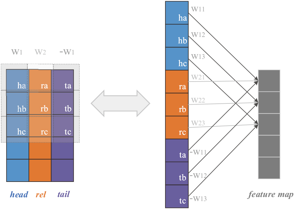

The constraint on the convolution filter values in ConvUs ultimately ensures its uniformity. In Eq. (3), since the signs of the two rows corresponding to head and tail embeddings in the filter are opposite, the relationship between the transformed entity embeddings is still translation-like. By comparison, ConvUs essentially adds convolution-based identical transformations for head and tail embeddings and unique transformations for relation embeddings to the translational relationship in TransE. The similarities and differences with the standard translational relationship ensure that the association between head and tail embeddings in ConvUs remains additive rather than projective, and the identical transformation on head and tail embeddings keeps their embedding spaces synchronised; uniformity is thus established. The unique transformations for relation embeddings project them to an additional embedding space, which is consistent with our definition of uniformity in Section 3.1 and can effectively enhance the model’s expressiveness.

In the implementation, we use trainable tensors ${\bm{\omega}}_{1}$ and ${\bm{\omega}}_{2}$ and stack them according to Eq. (2) to form the convolution filters, ensuring that the convolutional operations on the head and tail entity embeddings remain consistent after parameter initialization and the updates for each epoch.

3.3 Multi-scale, multi-layer CNN with L2 norm-based scoring function

After the convolutions on the stacked embeddings, the rich features in the original triple are extracted and multiple feature maps are generated. The plausibility score of each triple is derived based on the multiple feature maps. Another important aspect of ensuring uniformity in ConvUs is the improvement in the triple scoring process in ConvKB. We mentioned that using a fully connected layer to compute the score is insufficiently reasonable. Therefore, we propose a multi-scale, multi-layer CNN architecture with a non-parametric L2 norm-based scoring function, which does not introduce unnecessary dimensional interactions for uniformity and provides exceptional expressiveness. Specifically, following the filter-constrained convolutions, the convolutions are continued. With multiple layers of convolution, a unique feature map (i.e. the feature vector) ${\bm{v}}^{l}\in\mathbb{R}^{k^{l}}$ is obtained, which is then fed into a non-parametric scoring function to achieve the final score for each triple. In this section, we describe the multi-scale multi-layer convolution network and the L2 norm-based scoring function used in our model.

3.3.1 CNN architecture

A multi-layer CNN is used in ConvUs for the following two reasons: first, to extract deep features of the triples and better exploit the expressiveness of CNN and second, to gradually obtain a unique output feature vector $v^{l}$ where the correspondence with the dimensions of the original embeddings is established. Because the feature maps obtained after the first 2D convolutional layer are multiple vectors, 1D convolutions are introduced as the subsequent convolutional layers. The multiple convolutional layers are progressively distilling the feature maps, and each layer of convolution is a refinement of the triple features. After the final convolutional layer, the unique feature vector ${\bm{v}}^{l}$ is output, in which the semantic features of the corresponding triple are fully extracted.

For the scale of the filters in the convolution network, different filter lengths play different roles in processing the inputs of each convolutional layer. A convolution filter of length 1 interacts only on dimensions at the same position in different embeddings or feature maps, that is, modelling only heterogeneous interactions. By contrast, a longer convolution filter involves modelling both homogeneous and heterogeneous interactions. The longer the length of the convolution filter, the greater the weight of the homogeneous interactions modelled, and the larger the perceptual field of the convolution network. Based on the standard translational relationship, convolution filters of length 1 should be included in all convolutional layers as this class of convolutions models only heterogeneous interactions, which is most similar to the form of TransE and theoretically better inherits the nature of TransE. Convolution filters longer than one are also necessary to enable the model to represent homogeneous interactions and thus become more expressive. This is particularly true for modelling the association of relation embeddings with entity embeddings, which should not be limited to dimensions at the corresponding positions.

Therefore, when selecting the convolution filter length for each convolutional layer, instead of avoiding [10] or taking overly aggressive measures [9] to cope with different interactions between embedding dimensions, we aim to flexibly tune interactions at different scales through controllable convolution filter lengths and determine the most suitable embedding interactions for KGE. We are inspired by Inception [21] and adopt multiple convolution filter lengths and propose a paralleled mechanism to assign convolution filters with different lengths to the inputs of each convolutional layer.

The proposed mechanism for the convolution with different length convolution filters in multiple layers is shown in Fig. 2. Instead of mixing all feature maps to perform multi-scale convolution, which tends to model numerous local homogeneous interactions within the embeddings and produces an insignificant number of pure heterogeneous interactions after multiple layers of convolution, our convolution network parallelises the convolutions of differently sized convolution filters, preserving more heterogeneous interactions and allowing for a more controllable allocation of the interactions at different levels.

Figure 2.

multi-scale convolution mechanism. The different coloured dashed boxes indicate convolutional filters of different lengths. After convolutions of the input, corresponding groups of feature maps are generated, distinguished by different colours. The convolutions of different feature map groups are paralleled and merged in the final convolutional layer to give a unique final feature vector.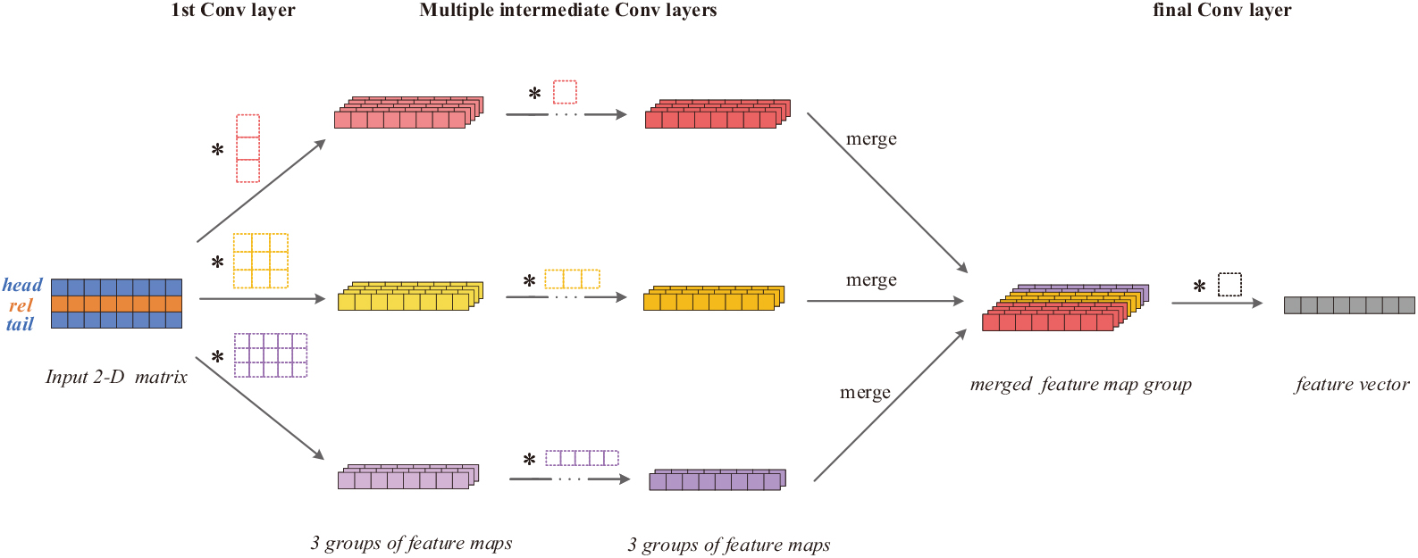

Considering the convolution filter lengths 1, 3 and 5 as an example. In Fig. 2, first, the multi-length convolution filters jointly interact in the input 2D matrix. After generating the three groups of feature maps, the convolution filters with certain lengths in the subsequent layers only operate on the corresponding same-length feature map groups. As the convolution proceeds, the number of output feature maps gradually decreases as the depth of the convolutional layers increases. After several feature extractions, the last convolutional layer merges all feature map groups before conducting convolution to obtain a unique feature map group. Only a single length-1 convolution filter is used in the final convolutional layer, which yields the feature vector for triple scoring.

In the above paralleled multi-scale CNN architecture, with a fixed number of length-1 convolutional filters, a considerable number of output dimensions are derived only from the heterogeneous interactions. Additionally, this is an unambiguous and intuitionistic mechanism for assigning convolution filters of different lengths, where the proportion of interactions at different scales can be easily altered by adjusting the ratio of convolution filter lengths. This helps to achieve the most suitable proportion of interactions for modelling specific relation patterns and knowledge graphs, providing the model with a stronger generalisation. In Section 4.6, we briefly compare and analyse the effect of the heterogeneous and homogeneous interactions by adjusting the ratio of different convolution filter lengths.

3.3.2 Scoring function

The computation of the triple score is essentially a dimensionality reduction of the feature map( $s:\mathbb{R}^{M^{1}k^{1}}\rightarrow\mathbb{R}^{1}$ , $M^{1}$ and $k^{1}$ are respectively the feature map number and dimensionality at the end of the first convolutional layer), where the interactions between dimensions of the same embedding are inevitable. However, not all homogeneous interactions are unnecessary, except those modelled by fully connected layers are often difficult to control due to their large number of parameters. We aim to minimise the number of unnecessary homogeneous interactions in the triple scoring function, ensuring that the interactions modelled do not destroy the uniformity of the entity embedding space. In ConvUs, the scoring function used is inspired by TransE.

In TransE, head entities, relations, and tail entities are represented in the same embedding space. It is assumed that the difference between the sum of the head entity and relation embeddings and the tail entity embedding in an existing triple should be as small as possible. The magnitude of this difference is calculated as the triple score, which is measured in terms of the L1 norm or L2 norm as follows:

$\displaystyle S=\|{\bm{v}}_{h}+{\bm{v}}_{r}-{\bm{v}}_{t}\|_{2}$ (4)

Equation (4) is the scoring function in TransE based on the L2 norm. We introduce this concept to ConvKB by directly calculating the L2 norm of the feature vector from the final convolutional layer to score the triples:

$\displaystyle S=\|{\bm{v}}^{l}\|_{2}$ (5)

where ${\bm{v}}^{l}\in\mathbb{R}^{k^{l}}$ is the feature vector obtained from the final convolutional layer $l$ , which includes comprehensive information about the corresponding triple. Although this L2 norm-based scoring function would still result in heterogeneous interactions between the different dimensions of the input feature vector, these interactions are intuitive and not completely black box. In general, for the scoring function of ConvUs, to obtain a more accurate and simplified scoring of each triple, we disregard the expressiveness of the fully connected layer (compensated and even enhanced by the addition of the multi-layer, multi-scale CNN) and select a non-parametric form function to score triples, which is more in line with uniformity.

3.4 Orderliness contradiction and circular convolution

The aforementioned improvements enable ConvUs to model entity embeddings in a uniform space. We next focus on a potential contradiction between uniform space KGE and the mechanism behind the CNN layers and find that traditional convolutional layers are not suitable for learning knowledge embeddings. The starting point of this observation is that the operation of traditional convolutional layers is ordered, as reflected in the following two characteristics possessed by convolutions:

1) 1.
Local interactions are modelled with priority in the convolutions. For example, when a convolution filter of length 3 is used to operate on the input data, most of the operations are built between each input dimension and its most adjacent dimensions covered by a single convolutional filter. In contrast, although the perceptual field of the convolution network can be extended by stacking multiple convolutional layers and constructing the interactions of each dimension with more distant dimensions, the number of these global interactions is significantly smaller than that of the interactions established in a local sense. Therefore, CNNs tend to build local interactions within a small range on the input, which makes them better at coping with small-scale dense information when processing image or text information, such as the recognition of specific objects in complex images and the extraction of specific word fragments in long texts.

Figure 3.
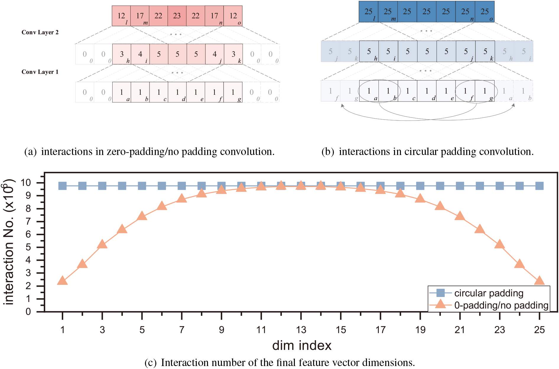
(a) and (b) refer to the interactions in convolutional layers with 0-padding or no padding and circular padding respectively. Each block represents a dimension. The letters in the lower right corner of the blocks indicate the index of the dimensions, while the number on the blocks and the colour depth of them represent the number of interactions involved in deriving these dimensions. The light-coloured blocks in the dashed border represent the padded dimensions. Interactions of dimensions are increased after convolutional layers and are uneven in 0-padding/no-padding convolution. (c) is the interaction numbers of each dimension after 10 convolutional layers of filter length 5. Differently coloured lines stand for the network using different padding methods.

2.
In traditional convolutional layers, features close to border locations are usually convolved differently, that is, they are exposed to fewer effective interactions and have smaller perceptual fields. For example, when no padding or zero padding is involved, the boundary dimensions establish interactions with only some of the other dimensions. Thus, the number of effective interactions engaged by the boundary dimensions in a single convolutional layer is smaller than those of the other dimensions (as shown in Fig. 3(a), the difference depends on the convolution filter length). As the CNN deepens, the difference between the number of interactions of the boundary and other dimensions expands; adjacent dimensions closer to the centre dimension are also affected and have fewer interactions than the centre dimensions. Figure 3(c) shows the difference in the number of interactions with different padding methods after a 10-layer convolution network. This characteristic of convolutions makes the features close to border locations in the input data different; therefore, CNNs should be used to process input data with boundary specificity, such as images or text with explicit boundaries.

The above two characteristics make the convolutional layer operate on the input dimensions in an ordered and locally relevant manner. However, considering the uniformity in TransE and the nature of representation learning, the dimensions in the embedding space should have unique implicit semantics, with no innate tendency towards a specific order. Specifically, both the local correlation between adjacent dimensions and the boundary dimension specificity are not inherent characteristics of the embeddings of knowledge graphs. This orderliness contradiction makes traditional convolutions intrinsically attach meaningless and unnecessary constraints to the representation learning when applied to such data, limiting the expressiveness of the model and embeddings.

Measures should be taken to address the above orderliness contradiction. Local interactions between dimensions can be reduced by increasing the length of the convolution filter or by using a length 1 filter. The multi-scale convolution filters of length 5 and length 1 mentioned in Section 3.3 can alleviate this problem to some extent. In contrast, the specificity of the boundary dimensions should be eliminated by introducing new techniques. In ConvUs, circular convolution was used for filters of length greater than one in each convolutional layer, that is, padding the input vector (or matrix) with the values of entries at the end of the other side (as in Fig. 3(b). After the circular padding, the ends of the input data to the convolutional layer are connected to form a loop, where the boundary dimensions do not exist, and the convolutions is circulated between the dimensions. The effect of this is illustrated in Fig. 3(b). After multiple layers of convolution, the interaction numbers of each dimension of the input vector are identical, that is, all dimensions inside the input are convolved identically.
3.5 Overall scoring function and loss function

In summary, the overall scoring function of ConvUs is as follows:

$\displaystyle s(h,r,t)=\left|\left|\sigma\left(W^{3}\otimes\sigma\left(\sum% \limits_{j}^{M^{2}}W_{j}^{2}\otimes\sigma\left(\sum\limits_{i}^{M^{1}}W_{i}^{1% }\otimes[{\bm{v}}_{h};{\bm{v}}_{r};{\bm{v}}_{t}]+{\bm{b}}^{1}\right)+{\bm{b}}^% {2}\right)+{\bm{b}}^{3}\right)\right|\right|_{2}$ (6)

where $W_{i}^{l}\in\mathbb{R}^{y^{l}\times{z^{l}}},z^{l}\in{Z}$ ( $Z$ is the set of filter lengths, and $y^{l}$ is the filter width for each convolution layer: $y^{l}=3$ for $l=1$ , else $y^{l}=1$ ) represents the $i$ -th filter in the $l$ -th convolutional layer and $b^{l}$ is the bias in the $l$ -th layer. $W^{3}$ is the only length-1 filter in the final convolutional layer, generating a unique feature vector for triple scoring. $\sigma()$ are the activation functions, we recommend using Leaky ReLU as the activation functions $\sigma()$ , since it can prevent the neurons from ‘death’, which may lead to multiple zeros in the final scores of the triples and impact the evaluation of the model. The overall scoring function shows a 3-layer CNN architecture, with $M^{1}$ and $M^{2}$ being the overall filter number in the first layer and second layer. All convolution inside Eq. (6) is circular convolution as illustrated in Fig. 3(b).

Figure 4.

Overall network architecture. The dashed boxes represent the field covered by each filter size and the speckled blocks are padded dimensions. Embeddings of a certain triple are first stacked to get a 2-d matrix before being fed into the circular convolutional network. The convolution filters in the network are multi-scale and constrained in the first layer. Eventually, a unique feature vector is output and used to derive the final score via an L2 norm-based scoring function.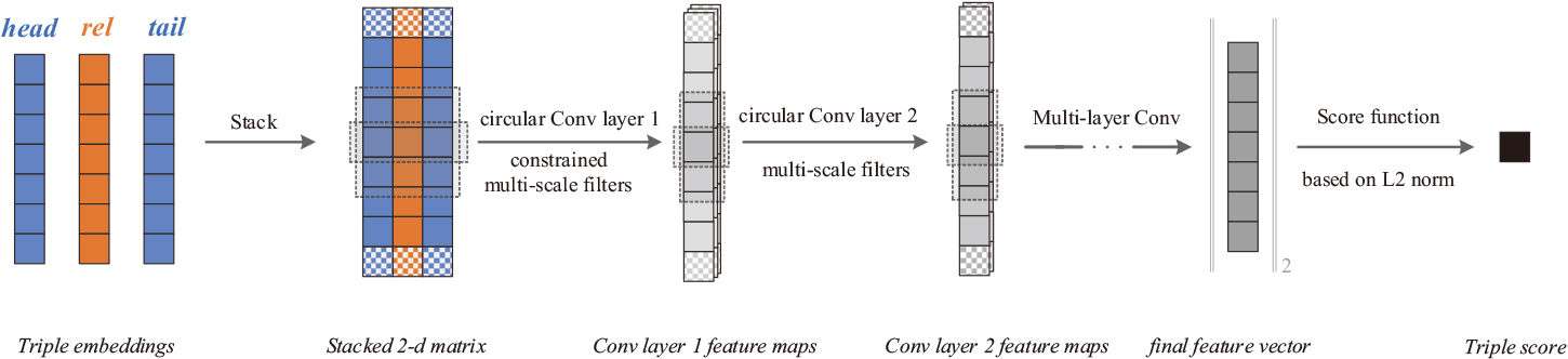

This scoring function is based on CNN and satisfies uniformity. We represent its corresponding overall model in Fig. 4. Embedding vectors of a certain triple are first stacked into a 2-D matrix, where the convolution operation with constraints is performed, giving birth to a number of 1-D feature maps. All feature maps are not injected into a fully connected layer, instead, they continue to be convolved using multi-scale convolutional layers. Among all convolutional layers, The convolution operations of multiple filter lengths are paralleled and circular convolutions are employed. A unique feature vector is extracted from the final convolutional layer. The score of the triple is computed directly from the L2 norm of the feature vector.

Embeddings and model parameters are updated during the training process, we use the margin-based loss function, following TransE, expressed as follows:

$\displaystyle\mathcal{L}=\sum\limits_{\left(h,r,t\right)\in{\mathcal{G}}}\sum% \limits_{\left(h^{\prime},r,t^{\prime}\right)\in{\mathcal{G}^{\prime}}}{\left[% \gamma+s\left(h,r,t\right)-s\left(h^{\prime},r,t^{\prime}\right)\right]_{+}}$ (7)

where $\mathcal{G}$ and $\mathcal{G}^{\prime}$ are the sets of positive and negative triples respectively, $\left(h^{\prime},r,t^{\prime}\right)$ refers to the unseen triple where the head or the tail entity is corrupted. $\gamma$ denotes the margin. $s()$ is the overall scoring function Eq. (6). $[\ ]_{+}$ filters the negative values.

4. Result

We conduct link prediction experiments to evaluate our model against multiple baseline models in datasets. We use the proposed overall scoring function in ConvUs to score candidate triples for link prediction.

4.1 Datasets

The link prediction performance of our model was evaluated on the WN18RR and FB15k-237 datasets, which are the improved versions of WN18 and FB15k, respectively. [22, 10] argue that WN18 and FB15k fit well with models that naturally capture the inverse relationship of the relations and this makes their prediction accuracy unreasonably high. Hence, the two original datasets failed to fully and correctly reflect the actual prediction ability of KGE models. To better evaluate the ability of KGE models, inversion relations were removed from both datasets to build WN18RR and FB15k-237. Table 1 shows the statistical information of the two datasets, where ‘rel./ent.’ is the ratio of relation number and entity number; ‘2-hop comp. rel.’ and ‘1-to-N/N-to-1 rel.’ is the rate the triples with 2-hop compositional relation (certain relations can be compositions of multiple relations, as in Fig. 7(a), 2-hop means the relation is composed of 2 sub-relations) and 1-to-N/N-to-1 relation respectively.

Table 1
Datasets information

Dataset	WN18RR	FB15k-237
Entities	40943	14541
Relations	11	237
Rel./ent.	2.69e-4	1.63e-2
Train triples	86835	272115
Valid triples	3034	17535
Test triples	3134	20466
2-hop comp. rel.	8.4%	13.3%
1-to-N/N-to-1 rel.	18.3%/46.8%	7.1%/19%

4.2 Training protocol

We trained the model parameters and embeddings for ConvUs based on the training triples on both datasets. The training of the KGE models aims at learning the underlying patterns of the knowledge graph based on existing knowledge triples and enables the model to determine the plausibility of unknown triples. Owing to the specificity of this task, a dataset for KGE models is essentially a list of existing triples within the knowledge graph, and the samples are not explicitly labelled. Therefore, to perform supervised training, the training triples should first be negatively sampled, that is, for each triple in the knowledge graph, the head and tail entities should be replaced with other entities sampled from the entity set to obtain a negative sample triple with a label of 0 (invalid triple), while the original valid triples are given a label of 1. Our negative sampling is based on the Bernoulli trick [15], and for each triple in the training set, we negatively sampled its head and tail entities to obtain the corresponding two negative samples. We trained the model parameters and embeddings based on the obtained positive and negative training samples, and the model hyperparameters were selected based on the link prediction performance (using the result of the mean reciprocal rank, MRR) of the model on the validation set. Following ConvKB, all entity and relation embeddings were first pre-trained with TransE with an embedding dimension of 100. Subsequently, mini-batch stochastic gradient descent was used to train our model, where the batch size was set to 128. For each batch of data, we first look up the current embeddings of each triple and then input them into the model to compute the triple score. After that, we substituted the corresponding positive and negative triple scores into the loss function Eq. (7) and optimised the parameters and embeddings using Adam optimisation so that all positive samples tended to have a low score, and all negative samples tended to get a high score. The learning rates we used on WN18RR and FB15k-237 were 5e-5 and 1e-8, respectively.

For the scale of our network, overall five layers were employed to perform the feature extraction, where the filter numbers were gradually decreased as 300/160/80/30/1 (for WN18RR) and 80/60/40/35/1 (for FB15k-237). In experiments on WN18RR, except for the last convolutional layer, each convolution was performed with filters of multiple lengths (1, 3, and 5), with a filter length ratio of 0.5:0.3:0.2, which was designed to increase heterogeneous and homogeneous interactions at a local scale. While for FB15k-237, we used only filters of length 1.

During training, each filter was initialised using a modified version of the He initialiser [23] since we used a leaky rectified linear unit as the activation function. The proposed initialiser used both fan in and fan out to calculate the standard deviation (in a convolutional layer fan in refers to the input depth whereas fan out is the output depth):

$\displaystyle\textit{stddev}=\sqrt{\frac{4}{\left(\textit{units\_in\_filter}% \cdot\left(\textit{fan\_in $+$ fan\_out}\right)\right)}}$ (8)

4.3 Evaluation protocol

We evaluated the performance of the KGE models using test triples in the corresponding datasets. In line with existing work, the performance of ConvUs was evaluated by making the predictions for the head and tail entities separately and averaging the results from both predictions. Specifically, for each test triple, we replaced the head and tail entities with other entities to form two sets of candidate triples for scoring. Unlike the negative sampling in training, which replaced only one (or a small number of other entities) of the head and tail entities of the correct triple, the entities used for replacement in the evaluation process included all other entities except those that potentially form existing triples of the corresponding knowledge graph (the ‘filtered’ setting protocol [4]).

We applied lookup on the well-trained embeddings for each candidate triple and then entered them into ConvUs to obtain the corresponding triple scores. The scores of candidate triples in each set were sorted to achieve the rank for each candidate triple (especially for the positive one) to calculate three evaluation metrics: the mean rank (MR) of the positive triple out of all the triples in the batch, where lower is better; the mean value of the reciprocal rank (MRR) of the positive triple out of all the triples in the batch, where higher is better; and Hits@N, which is the ratio of positive triples ranking less than or equal to N, where higher is better. All metrics (including different values of N) show the different aspects of the link prediction ability of KGE models.

4.4 Main results

Table 2
Head/tail/average evaluation results on benchmark WN18RR

Metrics	MR	MRR	H@10	H@3	H@1
TransE	2166/2635/2401	0.25/0.21/0.23	0.54/0.48/51	0.38/0.35/0.37	0.07/0.03/0.05
DistMult	7050/7140/7090	0.45/0.41/0.43	0.50/0.48/0.49	0.46/0.44/0.43	0.42/0.38/0.40
ComplEx	7710/6400/7060	0.45/0.44/0.44	0.52/0.50/0.51	0.46/0.45/0.45	0.42/0.41/0.41
SimplE	-/-/8764	-/-/0.40	-/-/0.42	-/-/-	-/-/0.38
R-GCN	-/-/2743	-/-/0.22	-/-/0.51	-/-/0.37	-/-/0.04
ConvKB	2762/2723/2743	0.24/0.21/0.22	0.53/0.49/0.51	0.39/0.36/0.37	0.05/0.03/0.04
ConvUs	915/623/769	0.44/0.38/0.41	0.59/0.50/0.55	0.49/0.42/0.46	0.35/0.31/0.33

Table 3

Head/tail/average Evaluation results on benchmark FB15k-237

Metrics	MR	MRR	H@10	H@3	H@1
TransE	311/141/226	0.39/0.19/0.29	0.60/0.35/0.47	0.44/0.21/0.32	0.28/.10.19
DistMult	-/-/254	-/-/0.24	-/-/0.42	-/-/0.26	-/-/0.16
ComplEx	414/410/412	0.35/0.17/0.26	0.55/0.36/0.46	0.41/0.22/0.32	0.29/0.13/0.21
SimplE	-/-/-	0.18/0.13/0.15	0.33/0.25/0.29	0.19/0.14/0.17	0.11/0.08/0.09
R-GCN	-/-/196	-/-/0.27	-/-/0.46	-/-/0.29	-/-/0.17
ConvKB	287/121/204	0.40/0.20/0.30	0.60/0.37/0.48	0.44/0.22/0.33	0.30/0.12/0.21
ConvUs	508/175/342	0.40/0.20/0.30	0.58/0.35/0.47	0.44/0.22/0.33	0.30/0.12/0.21

The baseline models in our experiment were TransE, ConvKB, DistMult, ComplEx, SimplE, and R-GCN, among which ConvKB is the very base model of ConvUs. The overall experimental results of all models on WN18RR and FB15k-237 are shown in Tables 2 and 3 respectively. The results for TransE are from the implementation of OpenKE [24] available at https://github.com/thunlp/ OpenKE/tree/OpenKE-Tensorflow1.0; the results of SimplE, ComplEx, and R-GCN are from the implementation available at https://github.com/zjukg/NeuralKG; the results of DistMult from the implementation available at https://github.com/uclnlp/inferbeddings; and the results for ConvKB were re-evaluated using the latest PyTorch implementation provided by the official ConvKB code available at https://github.com/daiquocnguyen/ConvKB.

Compared with the base model ConvKB, ConvUs achieved better results overall. Its superiorities are distinctly demonstrated by the experiment on WN18RR benchmark, where its results for all metrics outperformed ConvKB for both head and tail entity predictions. In particular, ConvUs significantly outperformed ConvKB by about 0.19 in MRR; the MR of the positive triples in the experiment also increased by almost 2000 places, indicating the huge performance improvement achieved by ConvUs. For Hits@10, where ConvKB is the most dominant, the results of ConvUs still improved by 0.04 (the average value for head and tail prediction). The original ConvKB paper does not report the results for Hits@1 and Hits@3, which are important prediction performance metrics. Based on the latest official PyTorch implementation of ConvKB, we performed a complete evaluation of ConvKB. The results show that the average prediction performances of Hits@1 and Hits@3 on the WN18RR dataset were at 0.04 and 0.37, respectively, which are approximately 10% and 80% of ours, respectively. Generally, the main improvement of ConvUs over ConvKB lies in the high accuracy metrics, indicating that it is more likely to make accurate link predictions than the base model.

When compared with other models, ConvUs also performed well, demonstrating its superiority in its uniformity and high expressiveness. As the most basic translational model, TransE fully satisfies the uniformity concept, and thus its results were relatively good on FB15k-237. However, it was still inferior to our model on both datasets owing to its insufficient expressiveness. Despite their greater expressiveness, SimplE and R-GCN lacked consideration for uniformity and do not have a uniform embedding space for entities or relations; therefore their performance is not ideal. DistMult and ComplEx conform to uniformity to some extent and are highly expressive. Therefore, they performed remarkably well on WN18RR, but their performance on FB15k-237 was lower than ConvUs. Moreover, it is worth mentioning that, with respect to MR on WN18RR, ConvUs dramatically outperformed all other models. In general, because ConvUs incorporates the characteristics of uniform space embedding from the translational relationship and the high expressiveness from the CNN, it performs well across metrics and datasets, making it rich in practical applications, generalisable, and able to achieve superior results on specific metrics and datasets while taking full advantage of its underlying strengths. We analyse this characteristic of ConvUs in the next section.

4.5 Extended analysis

We note that in the results in Tables 2 and 3, the two models that incorporate the idea of translation, ConvKB and TransE, tend to differ significantly from the other models in the distribution of the experimental results. From this observation, we alternatively divide the existing models into translation-like models (including translational models and other models that apply translation ideas, such as ConvKB) and non-translation-like models (other models that do not apply translation ideas) based on whether or not they contain the idea of the translational relationship. Further experiments were conducted to compare ConvUs with these two types of models to analyse the in-depth advantages and a potential trade-off that ConvUs offers.

4.5.1 Metrics analysis and applicability of ConvUs

Different metrics for link prediction reveal the applicability of KGE models to different types of practical applications. We first focus on the propensity of the two types of models with respect to different metrics, analyse the potential role of uniformity behind this propensity, and compare their results with those of ConvUs to confirm its better applicability.

Figure 5 shows the Hits@N results for each model at different N. One significant trend is that translation-like models usually yield better results at larger N. They can easily narrow down the scope of the correct triples (we refer to this type of prediction as fuzzy prediction). However, these models are limited when N is very small, which is an important limitation of models such as ConvKB in practical applications. By contrast, non-translation-like models have a higher hit rate when N is small, which makes them better at accurate prediction, but they cannot score reasonably well in widespread cases when an accurate prediction fails to be made.

The reason behind this phenomenon is that the translation-like models use uniformity as the underlying rule, ensuring that it is always able to carry out the triple scoring with a degree of rationality; a non-translation-like model does not have the support of uniformity but is able to fit some of the relations with a high level of accuracy because of its high expressiveness.

Figure 5.

Comparison of two classes of models and ConvUs for different metrics. The lines indicate the Hits@N results of the models for different N values; the different lines represent the different KGE models.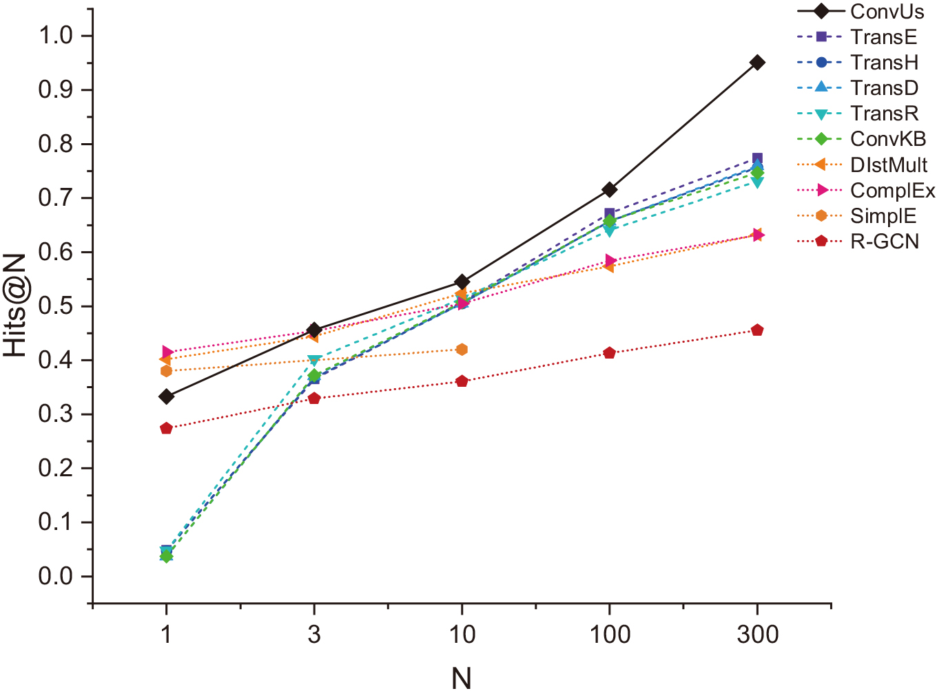

We now compare the two types of models with ConvUs. The line of ConvUs in Fig. 5 shows that, because it is a uniform CNN-based model, it combines the advantages of both types of models. The accurate prediction ability (Hits@1 and Hits@3) of ConvUs reaches the level of non-translation-like models and is much higher than that of translation-like models such as ConvKB. With respect to fuzzy prediction ability (Hits@10 or an even larger N), ConvUs performs significantly better than all models including translation-like models. This indicates that ConvUs is able to accurately predict both head and tail entities while ensuring that triple scoring is reasonable in most cases. It hence has applicability in more types of application scenarios.

4.5.2 Datasets analysis and generalization of ConvUs

Furthermore, we visually compare the performance differences among the comparison models and ConvUs on different datasets, discuss the reasons behind these differences, and highlight the generalization of ConvUs.

Figure 6.

(a) and (b) refer to the Hits@3 and Hits@10 results of two classes of models and ConvUs on WN18RR and FB15k-237. The color of the bars represents the different datasets.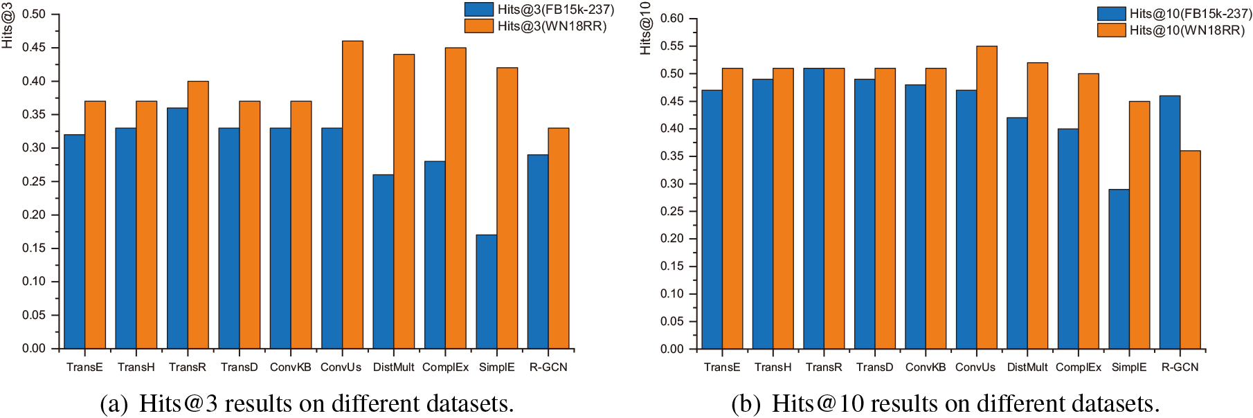

In Fig. 6, we show results for moderate values of N (Hits@3 and Hits@10) to illustrate the performance of each model on different datasets. It can be seen that although for any given model, the prediction results on the WN18RR dataset are generally better than those on the FB15k-237 dataset, when comparing the two types of models, translation-like models typically perform better on the FB15k-237 dataset, whereas non-translation-like models perform better on the WN18RR dataset.

The intrinsic reason for this variability lies in the different distributions of the relation patterns in the two datasets and the difference in the difficulty of relation pattern modelling in the two types of models. We further explain these reasons from the perspective of the dataset and model separately.

Considering the datasets, a major difference between FB15k-237 and WN18RR is the number of relations–FB15k-237 has 237 relations, whereas WN18RR has only 11 relations. This results in a significant difference in the distribution of relation patterns between the two. FB15k-237, due to its high number of relations, will inevitably lead to the compositions of relations, that is, the occurrence of compositional relations; as for WN18RR, given the small number of entities involved, is likely to have more 1-to-N, N-to-1 relations that are shared by multiple head or tail entities. Detailed statistics of these relation patterns are shown in Table 1.

From the perspective of the model characteristics, we have mentioned that translation-like models typically establish a uniform embedding space in which the various associations between entity and relation embeddings are represented as geometric relationships (strictly speaking, for many translation-like models, this geometric relationship is established between embeddings after certain projections). This confers inherent advantages in modelling compositional relations, as compositional relations in knowledge graphs are very similar to the geometric relationships between entity and relation embeddings in a uniform space as a matter of form (as shown in Fig. 7(a) and 7(b)). This enables these models naturally model compositional relations. The FB15k-237 dataset contains richer compositional relations, and thus translation-like models usually perform better in prediction on this dataset. However, translation-like models are commonly very simple, and many of them model both entities and relations in the same space. Although these characteristics help establish the geometric relationships, they also severely limit the models’ expressiveness, making it almost impossible for them to model 1-to-N and N-to-1 relations (as shown in Fig. 7(c) and 7(d). The 1-to-N relation cannot be equal to all the differences between the head and tail embeddings at the same time.). Therefore, relatively speaking, non-translation-like models with enhanced expressiveness are more likely to model the large number of such relations present in WN18RR.

Figure 7.

(a) and (c) is the subgraphs involving relations of certain patterns, where the nodes represent entities and the edges represent relations, which together form multiple triples; (b) and (d) visualise the corresponding relation and entity embeddings in the embedding space (assumed to be projected to a 2-D space), where the arrows originating from the origin indicate the entity embedding vectors, while the other arrows indicate the relation embedding vectors or the differences between different entity embedding vectors. (a) and (b) correspond to the compositional relations where sub-rel 1 and sub-rel 2 jointly form comp-rel 2 while (c) and (d) correspond to the 1-to-N relation such as ‘comprise’.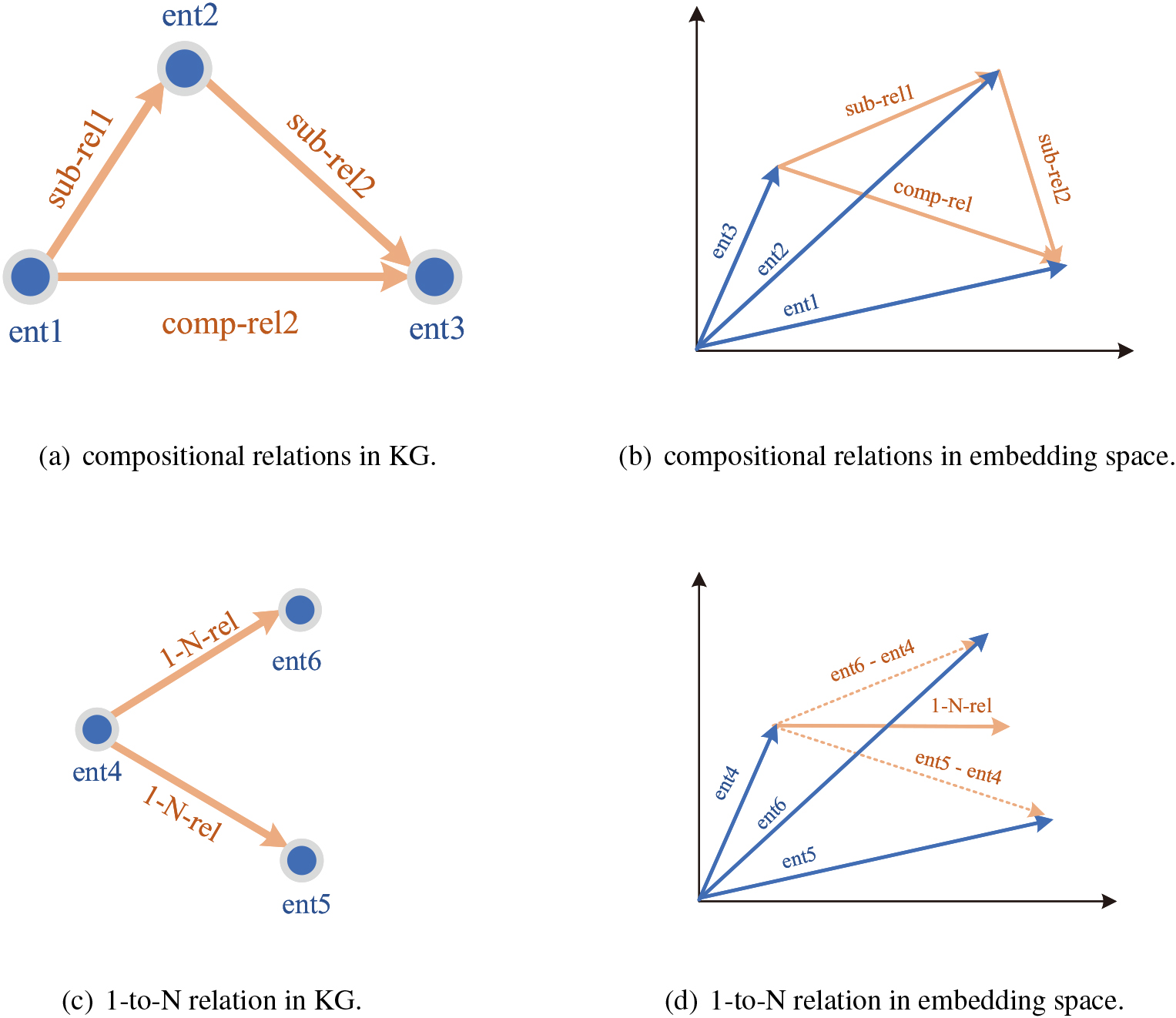

As in Fig. 6, although both types of models exhibit strengths on FB15k-237 and WN18RR for the reasons mentioned above, they show a lack of generalisation when compared with ConvUs. This is because ConvUs establishes a uniform entity embedding space onto which its relation embeddings are projected to form a geometric relationship with the entity embeddings. Therefore, it also has an advantage in modelling compositional relations. Meanwhile, the filters corresponding to the relation embeddings in ConvUs are unconstrained, in contrast to the constrained filters for entity embeddings (as shown in Eq. (3)). This improved expressiveness for relation embeddings, amplified by multi-layer nonlinear CNN, allows ConvUs to fully model 1-to-N and N-to-1 relations. Taking the two points above together, ConvUs is able to take into account the advantages of both types of models, thus surpassing all non-translation-like models on the WN18RR dataset and maintaining ConvKB’s leading position on the FB15k-237 dataset.

4.5.3 Inferiorities and superiorities in specific metrics

The above experiments demonstrate that, compared to other models, ConvUs has a notable advantage in its applicability to different application scenarios and generalization to different datasets. However, its results for specific metrics on these datasets may also reveal some minor inferiorities and pronounced superiorities in specific individual metrics on these datasets.

Inferiorities

It should be acknowledged that on the FB15k-237 dataset, although the results of ConvUs are relatively close to those of ConvKB, there are slight decreases in some metrics. This is essentially a trade-off made by ConvUs to enable it to comprehensively model the different relation patterns in the two datasets. That is, ConvUs has compromised its ability to model compositional relations to increase its expressiveness for 1-to-N and N-to-1 relations. Although ConvUs establishes a uniform entity embedding space and its relations are formally close to a standard translational relationship, they differ in certain ways from the original translation relations. For instance, it forgoes modelling both entities and relations in a uniform space and adopts multi-layer, non-linear CNNs in its triple score calculation. These measures weaken the geometric relationships between embeddings, which is detrimental to modelling compositional relations but substantially improves the modelling of 1-to-N and N-to-1 relations. As a result, the prediction performance of ConvUs decreases slightly on FB15k-237 but substantially improves on WN18RR, showing far better generalization than ConvKB.

Superiorities

ConvUs can also exhibit outstanding performance in individual metrics of certain datasets. Figure 5 reveals that for N greater than 10, ConvUs performs far better than other models on the WN18RR dataset, indicating that ConvUs is more capable of achieving a referenceable scoring of triples in almost any case, which naturally contributes to the smaller MR of the positive triples in the evaluation on WN18RR. We consider this phenomenon reasonable given all the above comparison results of ConvUs and the two classes of models. ConvUs benefits from the high hit rate of the translation-like models at larger N on the one hand, and from the advantages of the non-translation-like models in modelling the data in WN18RR on the other hand. These factors correspond to the two key features of ConvUs in principle – uniformity and strong expressiveness, respectively. Therefore, the superiorities of ConvUs in its fuzzy prediction on WN18RR data fully reflect the effectiveness of its core idea.

In summary, the superiorities and inferiorities of ConvUs revealed by individual metrics of certain datasets highlight its core strengths in terms of uniformity and expressiveness as well as its inadequacy in modelling compositional relations when compared with some translation-like models. Future research could explore ways to enhance the model’s expressiveness while ensuring its ability to model compositional relations. Notably, any improvement should be based on the foundation of uniformity.

4.6 Ablation study

Table 4
Ablation study results on WN18RR

Ablations	MRR
ConvKB	0.220
w/o filter value constraint	0.255
w/o circular convolution	0.403
w/o L2-based scoring	0.230
w/o filter length-3&5	0.245
w/o filter length-5	0.402
full ConvUs	0.410

We also conducted ablation experiments on ConvUs to evaluate the independent impact of our improvements based on the MRR metric on WN18RR. The ablations include the following:

•

ConvUs w/o filter value constraints: removing the constraints on filter value in the first convolutional layer of ConvUs. All entries in the filters are learned independently.

•

ConvUs w/o circular convolution: using 0-padding instead of circular padding before the convolution in each layer to avoid dimension reductions in each layer.

•

ConvUs w/o L2-based scoring: using a fully connected layer to achieve the triple score. To obtain enough neurons to perform fully connected layer projection, a single convolutional layer with 300 convolution filters is employed.

•

ConvUs w/o filter length-3&5: using a single filter of length 1 in each convolutional layer.

•

ConvUs w/o filter length-5: using only filters of lengths 1 and 3 in each convolutional layer. The filter ratio is 0.6:0.4.

The experimental results are shown in Table 4, where the performance of each ablation decreased after the corresponding improvement in ConvUs was removed. Ablations such as ConvUs without the filter value constraint, and ConvUs without filter length-3 & 5 resulted in a significant decrease in the performance of the model. As our main improvements, they have a great impact on the model performance. Additionally, we speculated that the large gap was due to the strong coupling between different improvements we made, that is, the removal of a specific improvement may affect the overall mechanism behind the model and thus lead to more significant performance degradation.

In contrast, because circular padding has a relatively independent effect on the model and is not subject to other uniformity-related improvements, the MRR result of ConvUs without circular convolution (using 0-padding instead) was the closest to the proposed ConvUs. However, the model still showed a performance degradation of 0.007 compared to full ConvUs, indicating that circular convolution is an effective and necessary improvement for enhancing the performance of the CNN-based KGE models.

The results further reveal that ConvUs without L2-based scoring is the model most similar to the original ConvKB, which contains only a single layer of convolution and uses a fully connected layer to calculate the triple score. In this case, the model no longer fully conforms to uniformity and the expressiveness is reduced by the decrease in the number of layers and scales, its MRR result was thus lower, reflecting the superiority of a multi-layer CNN architecture with the L2 norm-based scoring function.

Finally, using the parallel multi-scale convolution mechanism described in Section 3.3, we can visualise the effect of different interaction ratios on the prediction results of the model. The results of the last two ablations reveal that different convolution filter length configurations had a significant impact on the model performance, which inherently reflects the distinct effects of homogeneous and heterogeneous interactions on KGE. For experiments on WN18RR, the lower evaluation results of ConvUs without filter length-3 & 5 indicate that homogeneous interactions are critical in modelling the knowledge graph of WN18RR. However, such a conclusion does not apply to the knowledge graph of FB15k-237, where we obtained a better result when only length-1 filters were employed. This is reasonable when we consider that both ConvKB and TransE – the models focusing on establishing heterogeneous interactions – achieved better results on FB15k-237. Heterogeneous interactions accompanied by large scale convolutional filters bring about more transformational variability between entity and relation embeddings, making it difficult for relation embeddings to form geometric relationships with entity embeddings and detrimental to modelling the dominant compositional relations in FB15k-237. That is, the modeling of two types of interactions is also a factor in the propensity of translation-like and non-translation-like models for the two datasets as it affects the geometric relationship between embeddings. ConvUs can flexibly adjust the weight of different interactions, so it will not be affected by this point, which provides it with the potential to generalise more data.

4.7 Comparison on head and tail prediction

Additionally, in Tables 2 and 3, we provide the performance of each model for the specific tasks of the head entity and tail entity prediction, aiming to uncover insights behind their results. It can be observed that ConvUs, consistent with existing models, exhibit a tendency towards tail entity prediction, which makes it more valuable in application scenarios that emphasise tail entity prediction. One of the important reasons for this phenomenon is the widespread presence of 1-to-N and N-to-1 relations we mentioned in 4.5.2 and the imbalance in their quantities. For triples with 1-to-N relations, the distribution of head entities is more concentrated, making their prediction often easier than that of tail entities. Conversely, for triples with N-to-1 relations, tail entities are easier to predict than head entities. Moreover, in most knowledge graphs, the number of N-to-1 relations is usually greater than the 1-to-N ones (as in Table 1). Consequently, during comprehensive link prediction evaluations, the influence of N-to-1 relations becomes more pronounced, resulting in a higher level of difficulty for head entity prediction compared to tail entity prediction.

5. Conclusion

This study proposed ConvUs, a novel CNN-based knowledge graph embedding model that expressively represents all entities of a specific knowledge graph in a uniform space. The main improvements were made to introduce uniformity into ConvKB. With value-constrained convolution filters, a multi-layer, multi-scale convolution network, and L2 norm-based scoring function, ConvUs identifies the uniformity of an entity embedding space. It further incorporates the concept of circular convolution, aiming to alleviate the orderliness contradiction between uniform space KGE and traditional convolution.

Experiments on WN18RR and FB15k-237 illustrate that ConvUs achieved a better link prediction performance than the base model ConvKB and other baseline models which conform to uniformity and incorporate expressiveness to different degrees, ConvUs has the best overall performance, justifying the effectiveness of uniformity. Detailed comparisons of ConvUs with the various metrics results of translation-like models and non-translation-like models on different datasets served to further showcase the applicability and generalization of ConvUs while also highlighting its potential superiority and trade-off with respect to specific metrics of certain datasets. Finally, we also verified the effectiveness of the individual improvements on ConvKB through multiple ablation experiments. Some of the improvements in this study can be migrated to more CNN-based KGE models or other non-CNN models. Thus, the study provides a new perspective by introducing uniformity to enhance the link prediction performance of these models. Future work could focus on this or discover innovative approaches to enhance a model’s expressiveness while fully preserving its capacity for modelling compositional relations.

References

Lan

Jiang

Zhao

W.X.

Wen

J.-R.

, A survey on complex knowledge base question answering: Methods, challenges and solutions, In Proceedings of the Thirtieth International Joint Conference on Artificial Intelligence, IJCAI-21, 2021, pp. 4483–4491.

Chen

Zhang

Deng

Tan

Huang

Chen

, Hybrid transformer with multi-level fusion for multimodal knowledge graph completion, In Proceedings of the 45th International ACM SIGIR Conference on Research and Development in Information Retrieval, 2022, pp. 904–915.

Wang

Zhang

Pang

, Consensus-aware visual-semantic embedding for image-text matching, In Computer Vision – ECCV 2020: 16th European Conference, Glasgow, UK, August 23–28, 2020, Proceedings, Part XXIV, 2020, pp. 18–34.

Bordes

Usunier

Garcia-Duran

Weston

Yakhnenko

, Translating embeddings for modeling multi-relational data, Advances in Neural Information Processing Systems 26 (2013).

Yang

Yih

W.-T.

Gao

Deng

, Embedding entities and relations for learning and inference in knowledge bases, arXiv preprint arXiv:1412.6575, 2014.

Trouillon

Welbl

Riedel

Gaussier

É.

Bouchard

, Complex embeddings for simple link prediction, In International conference on machine learning, pp. 2071–2080. PMLR, 2016.

Kazemi

S.M.

Poole

, Simple embedding for link prediction in knowledge graphs, Advances in Neural Information Processing Systems 31 (2018).

Zheng

Shao

Yin

Liu

T.-Y.

, SEEK: Segmented embedding of knowledge graphs, In Proceedings of the 58th Annual Meeting of the Association for Computational Linguistics, 2020, pp. 3888–3897.

Nguyen

D.Q.

Nguyen

T.D.

Nguyen

D.Q.

Phung

, A novel embedding model for knowledge base completion based on convolutional neural network, arXiv preprint arXiv:1712.02121, 2017.

10.

Dettmers

Minervini

Stenetorp

Riedel

, Convolutional 2D knowledge graph embeddings, In Proceedings of the AAAI conference on artificial intelligence, volume 32, 2018.

11.

Huang

Zhang

Zhu

Tang

, A deep embedding model for knowledge graph completion based on attention mechanism, 33(15) (2021), 9751–9760.

12.

Schlichtkrull

, Kipf

Bloem

Berg

R.V.D.

Titov

Welling

, Modeling relational data with graph convolutional networks, In European semantic web conference, Springer, 2018, pp. 593–607.

13.

Nathani

Chauhan

Sharma

Kaul

, Learning attention-based embeddings for relation prediction in knowledge graphs, In Proceedings of the 57th Annual Meeting of the Association for Computational Linguistics, 2019, pp. 4710–4723.

14.

Fang

Zang

Wang

, A vectorized relational graph convolutional network for multi-relational network alignment, In Proceedings of the 28th International Joint Conference on Artificial Intelligence, 2019, pp. 4135–4141.

15.

Wang

Zhang

Feng

Chen

, Knowledge graph embedding by translating on hyperplanes. In Proceedings of the AAAI conference on artificial intelligence, volume 28, 2014.

16.

Lin

Liu

Sun

Liu

Zhu

, Learning entity and relation embeddings for knowledge graph completion, In Twenty-ninth AAAI conference on artificial intelligence, 2015.

17.

Liu

Zhao

, Knowledge graph embedding via dynamic mapping matrix. In Proceedings of the 53rd annual meeting of the association for computational linguistics and the 7th international joint conference on natural language processing (volume 1: Long papers), 2015, pp. 687–696.

18.

Yang

Tian

Zhang

Yan

Jin

, Transms: Knowledge graph embedding for complex relations by multidirectional semantics, In Proceedings of the 28th International Joint Conference on Artificial Intelligence, 2019, pp. 1935–1942.

19.

Zhang

Paudel

Zhang

Bernstein

Chen

, Interaction embeddings for prediction and explanation in knowledge graphs, 2019, pp. 96–104.

20.

Nickel

Tresp

Kriegel

H.-P.

, A three-way model for collective learning on multi-relational data, In Icml, 2011.

21.

Szegedy

Ioffe

Vanhoucke

Alemi

A.A.

, Inception-v4, inception-resnet and the impact of residual connections on learning, In Thirty-first AAAI conference on artificial intelligence, 2017.

22.

Toutanova

Chen

, Observed versus latent features for knowledge base and text inference, In Proceedings of the 3rd workshop on continuous vector space models and their compositionality, 2015, pp. 57–66.

23.

Zhang

Ren

Sun

, Delving deep into rectifiers: Surpassing human-level performance on imagenet classification, In Proceedings of the IEEE international conference on computer vision, 2015, pp. 1026–1034.

24.

Han

Cao

Lin

Liu

Sun

, Openke: An open toolkit for knowledge embedding, In Proceedings of EMNLP, 2018, pp. 139–144.

Knowledge graph embedding in a uniform space

Abstract

Keywords

1. Introduction

2.1 Translational models

2.3 CNN-based models

2.4 GNN-based models

3. Proposed method

3.1 Motivation

3.2 Convolutional filters with constrained values

3.3.1 CNN architecture

4.1 Datasets

Table 1 Datasets information

4.4 Main results

Table 2 Head/tail/average evaluation results on benchmark WN18RR

4.5.1 Metrics analysis and applicability of ConvUs

4.6 Ablation study

Table 4 Ablation study results on WN18RR

5. Conclusion

References

Table 1
Datasets information

Table 2
Head/tail/average evaluation results on benchmark WN18RR

Table 4
Ablation study results on WN18RR