We propose novel approaches for classification from positive and unlabeled data (PUC) based on maximum likelihood principle. These are particularly suited to measurement tasks in which the class prior of the target object in each measurement is unknown and significantly different from the class prior used for training, while the likelihood function representing the observation process is invariant over the training and measurement stages. Our PUCs effectively work without estimating the class priors of the unlabeled objects. First, we present a PUC approach called Naive Likelihood PUC (NL-PUC) using the maximum likelihood principle in a nontrivial but rather straightforward manner. The extended version called Enhanced Likelihood PUC (EL-PUC) employs an algorithm iteratively improving the likelihood estimation of the positive class. This is advantageous when the availability of the labeled positive data is limited. These characteristics are demonstrated both theoretically and experimentally. Moreover, the practicality of our PUCs is demonstrated in a real application to single molecule measurement.
Classification from positive and unlabeled data (PUC) [7, 27] has been actively researched in recent years. PUC is required in many problems where large amounts of unlabeled data are easily acquired but only limited quantities of one-class-labeled data are available. Many measurement tasks in scientific, industrial, and social sensing face such problems.
For example, the reinforced concrete in various real-world environments is classified as damaged or undamaged by ultrasonic testing [12]. The measurements of actually damaged samples are acquired from a limited number of past incidents, while many non-incident samples, which are either damaged or undamaged, are acquired without their labels. Similar situations are common in the field of industrial nondestructive inspection. Another example is the problem of classifying the risks of an individual suffering heart failure within the next 10 years based on cardiac function indices such as stroke volume (SV) and fractional shortening (%FS) which are geometrically measured by ultrasonic imaging [16]. Occurrences of heart failure are only recorded for persons who are actually hospitalized within the 10 years after their heart inspections, whereas most of those who are inspected but did not experience the heart failure remain unlabeled. Similar problems appear in other medical fields. As described later, some advanced scientific measurement such as single molecule measurement also includes the similar problem.
The problem setting underlying many measurement tasks, including these examples, is that we have a large data set of unlabeled samples and a small data set of other samples having positive labels such as “damaged” and “heart failure.” is drawn from the positive marginal density , and is from the marginal density:
where is the positive class prior probability . PUC learns a classifier from and , and this classifier can be used to obtain the measurement consequence.
A distinguishing feature of the measurement tasks is that and are defined by the sensing devices as likelihood functions of ; these functions are mostly invariant because the sensing devices are designed to preserve their characteristics for long periods to ensure high accuracy. In the aforementioned two examples, the ultrasonic sensors provide invariant likelihood functions on the concrete and the heart motion as long as they are well maintained. Another distinguishing feature of the measurement tasks is that the class prior probability of an individual target object or a set of target objects is unknown in each measurement and can be significantly different from the class prior probabilities of the objects targeted in other measurements. For instance, the prior probability of concrete damage deviates according to the real-world environment surrounding the individual concrete object. The prior probability of the heart failure is heavily dependent on the individual’s living environment. Thus, the problem setting underlying the measurement tasks can be more precisely stated as being that a newly measured sample follows the new marginal density
where an unknown prior probability can be very different from of used for the PUC training.
These arguments reveal difficulties to apply conventional PUCs to measurement problems [7, 27].
First, all past PUCs learn maximum a posteriori (MAP) classifiers in the standard setting of machine learning. A MAP classifier estimates the label assuming that is unchanged over the training and test (measurement) stages, and thus does not anticipate a large difference between and . This nature does not fit the aforementioned problem setting of the measurement tasks.
Second, all past PUCs require the availability of the class prior probabilities and before the training and test (measurement) stages [27] or a special labeling mechanism in the training data acquisition [7]. These requirements also do not meet the conditions of the measurement tasks.
In measurement tasks having the invariant and the large discrepancies between and unknown , the maximum likelihood estimation of from relying on the invariance of has been widely employed to avoid the above difficulty of the MAP approach, when both positive and negative labeled data sets: and are available for estimating [28]. However, to the best of our knowledge, there is no principle for accurately estimating from positive and unlabeled data sets: and without knowing . If maximum likelihood PUCs based on such a principle could be established, they would enable various new measurement tasks.
The contributions of the present study are as follows.
We propose the novel principle of maximum likelihood PUCs to address the aforementioned problems. These are the first PUCs that learn from the independently acquired two sample datasets: and and that do not require the estimation of the class prior probability.
The proposed PUCs are accurate even when a small labeled data set and a massive unlabeled data set are given, and thus have a practical advantage.
These characteristics and the statistical accuracies of the proposed PUCs are theoretically demonstrated.
We further show a feasible performance measure of the PUCs requiring positive and unlabeled data sets only. This measure can be used to select appropriate parameters for the PUCs in cross validation.
The performance of our proposed PUCs is confirmed through numerical experiments using artificial and benchmark data and a real-world application to noise reduction in advanced single molecule measurement.
Problem setting
Here, we define our problem setting more precisely. Let and be a sample in its domain and a positive () or negative () label, respectively. Given a training data set of unlabeled samples and a training data set of other samples having positive labels , let be an unlabeled test data set given by measuring new objects. may include only one sample, when the target object is unique. Samples in are i.i.d. sampled from the positive marginal density , and samples in and are i.i.d. sampled from marginal densities and , respectively. No negative data are given.
We now introduce two assumptions on .
.
, and share an invariant .
.
is positive and has bounded and continuous second derivatives on .
These are not special assumptions. All past PUCs assumed a common over all data sets [7, 27]. All past classifiers using a non-parametric estimation of the probability densities in a continuous space rely on Assumption 2. This assumption is used in a later section. From the first assumption, holds, and , consist of the common and the positive class prior probabilities and , respectively, as follows.
are unknown and independently given.
Our problem is to learn an accurate non-parametric classifier of unseen samples in the unlabeled test data set using only and . This is a two sample setting of PUC [27], whereas and follow mutually different unknown class prior probabilities.
Related work
There are two issues in tackling this problem. The first relates to the distinguishing feature of the measurement tasks such that no information about is known before classifying a sample in while its class prior can be significantly different from of . In the field of traditional classifiers that learn from both positive and negative labeled data, many approaches for adapting the classifiers to slight or gradual concept drift [8] and larger differences between the training and test data sets [19, 20] have been proposed. Classical semi-supervised classifiers that learn from small positive and negative labeled data sets and a large unlabeled data set are based on the transductive learning framework [29, 1], and the adaptation of the classifiers to different class prior distributions has been studied. Saerens et al. proposed a covariate shift adaptation for the difference in the class prior in the semi-supervised setting [22]. More recent study has proposed a transductive transfer learning method to estimate the change in the class prior under the same setting [5]. In the PUC setting, most of the conventional PUCs are unsuitable because they assumes an invariant as mentioned earlier. An exception is the PUC proposed by Li et al. which adapts to gradual changes in micro-cluster labels in a data stream [15]. However, all these approaches rely on the availability of a certain size of before classifying its samples or a gradual change in the class prior distribution of , and they are therefore not applicable to our problem.
The second issue comes from the fact that the values of and are unknown, while the training processes of many PUCs need these values. The past PUCs use one of the following two options to overcome this difficulty. The PUC of Elkan and Noto [7] uses an option called the one sample setting which assumes that and are identical, positive samples drawn from are labeled with a constant probability and included in , and the remaining unlabeled samples are included in [4]. This PUC implicitly estimates the class priors by partially matching the distribution of to that of . However, these assumptions are not always valid in measurement tasks where and are independently given and and are largely different. Some PUCs use the other option called the two sample setting which accepts independently acquired and [27, 6, 18]. This setting assumes that and are correctly estimated from , and by relying on irreducibility of that is not represented by a linear combination of and another probability density function of [2, 6, 23, 21]. However, this irreducibility is not generally guaranteed in measurement tasks. Moreover, is not usually available for estimating before the new measurement, and so cannot be applied to our problem setting.
In the next section, we propose two maximum likelihood PUCs not requiring in advance nor the estimation of and . Thus, they do not suffer the difficulties for the measurement tasks.
Proposed method and theoretical analysis
Naive Likelihood PUC (NL-PUC)
To design a PUC that is robust to differences between and , we employ the following maximum likelihood measure that does not depend on the class prior probabilities. According to Assumption 1, the maximum likelihood estimation of under is given as follows:
Associated with this measure, the following lemma holds.
.
Given a marginal density
the following inequalities are equivalent for any and X.
.
We obtain the following relation by substituting the definition of to .
From this lemma and Assumption 1, we immediately obtain the following, which is our core theorem.
.
For any combination of and in , the following formula is the maximum likelihood measure equivalent to Eq. (3) for all following .
.
From Eqs (1) and (2) and Lemma 1, the following holds:
Because the last inequality is independent of and according to Assumption 1, these three inequalities equivalently and invariantly hold for any and in . Equation (4) is therefore equivalent to Eq. (3), and the theorem holds.
We construct a maximum likelihood PUC by substituting the non-parametric estimations and derived from and , respectively, into this measure. They are provided by
where we use kernel densities such as Gaussian kernel which well approximates and under the condition of Assumption 2. We refer to this classification as Naive Likelihood PUC (NL-PUC).
Enhanced Likelihood PUC (EL-PUC)
Although NL-PUC satisfies our requirements, the classification may be degraded by large statistical errors in induced from the small size of , i.e., . To alleviate this difficulty, we estimate more accurately by iteratively improving using its linear combination with .
where and . is given by the following non-parametric approximation of using kernel densities and their weights . We use such as Gaussian kernel as well as in NL-PUC.
Their initial values are set as follows.
Equation (4.2) is a weighted non-parametric approximation of using the samples in and the normalized weights where follows and approximates defined by [26, 10]. Equations (6) and (7) further repeat the weighted non-parametric approximation of using its estimation from the previous step.
In the next subsection, we show that, if is of sufficient size and we choose an appropriate , the mean square error of can be no more than that of the non-parametric approximation directly derived from . Moreover, the mean square error of is limited under Assumption 2, because is positive and has bounded and continuous second derivatives on [24, 10]. Accordingly, converges to a value having better accuracy than . In practice, our numerical experiments show that using almost any widely gives a better estimation of than .
When the rate of change of converges within a small tolerance for all , we obtain a more accurate than given by NL-PUC, and apply to Eq. (4) with . This is called Enhanced Likelihood PUC (EL-PUC) and expected to have better accuracy particularly when is small.
Theoretical accuracy of EL-PUC
is positive and has bounded and continuous second derivatives on from Assumption 2, Eq. (1) and . Moreover, the size of is sufficiently large in most practical cases. Accordingly, the non-parametric estimation given by and used on the r.h.s. of Eq. (4) has a limited mean square error [24, 10]. Thus, we focus on the error of which is used on the l.h.s. of Eq. (4).
Let be the estimation of , be the absolute value of the bias , be the variance , and be the mean square error . Here, denotes the expectation over the distribution .
.
Let , then is bounded, and the following holds for .
.
From Eqs (6) and (7), is a weighted non-parametric approximation of . As in Eq. (4.2) is a linear combination of and which are positive and have bounded and continuous second derivatives by the use of the kernel density satisfying the condition of Assumption 2, the absolute expected error of against is bounded [24, 10]. Hence, is bounded for any , i.e., is bounded. Accordingly, by subtracting from both sides of Eq. (4.2) and taking their absolute expectations, the following holds.
By repeatedly applying this formula and applying in Eq. (4.2) when , we derive:
Moreover, the following holds.
By substituting the former inequality into this last line, we obtain our following result for .
This lemma shows that can be less than , if is sufficiently small.
.
The following holds for all .
.
By taking the expectation of Eq. (4.2) and subtracting it from Eq. (4.2) itself, we obtain the following for .
By taking the mean square of both sides, the following formula is derived.
According to the Cauchy-Schwarz inequality and the positivity of the variances, the underlined term is no more than . Thus the following inequality is obtained, and the lemma holds.
This lemma indicates that can be less than , if is sufficiently small. The following theorem is easily derived from these two lemmas.
.
If the following holds, there exists some such that .
hold. These facts imply that there exists some such that , if the differential of for is negative in a vicinity of , i.e.,
The above condition is equivalent to the following, which proves the lemma.
The variances of and obtained by non-parametric estimation using i.i.d. samples and weighted i.i.d. samples are known to be
respectively [26, 10, 14]. is a positive constant given by the integrated square of , and is the effective size of with weights defined as
From Eqs (1) and (7), in a certain fraction of have , and thus holds. According to this fact, Eqs (10) and (11), the r.h.s. of Eq. (2) is large, i.e., Eq. (2) may hold, when is small and is large. Therefore, when there are few samples in and many samples in , is generally less than if using an appropriate , and EL-PUC is expected to attain higher accuracy than NL-PUC.
This theoretical result is more intuitively explained by the nature of statistical bias end variance. The expectations of and do not mutually deviate significantly, since they are kernel based nonparametric estimations of . Thus, is small, and this ensures the small difference of the expected biases of and over the wide range of in Lemma 2. Whereas, the variance of is expected to be significantly larger than that of under the condition of , because they are dominated by and , respectively. In total, the mean square error of is less than that of .
Performance measure and parameter selection
When a certain amount of test data is available, the performance of our PUCs can be empirically evaluated for the purpose of comparison with other candidate PUCs and to tune the PUC parameters. However, standard performance indices such as AUC and F-measure are not applicable, because the test data sets in practical problems targeted by PUCs usually do not include labeled negative samples.
For such circumstances, a number of studies have proposed performance indices similar to the traditional AUC that assess the goodness of the classifier classes, but not particular parameter selections of the classifiers [9, 17, 11]. Only a few studies have proposed indices that are directly applicable to parameter selection. Lee and Liu proposed an index equivalent to the geometric mean of precision and recall in the one sample setting [13]. Calvo et al. proposed a generic pseudo F-measure that matches the traditional F-measure if we substitute the correct [3]. We employ the latter index because it is applicable to the two sample setting.
The unavailability of in our problems presents an issue. Given a labeled positive test data set and a unlabeled test data set with Assumption 1, assuming that both and have certain sizes for statistically stable evaluations, we derive the following lemma for our likelihood based PUC which uses Eq. (3) or equivalent Eq. (4). It ensures that the pseudo F-measure using an arbitrary in place of is a maximum if and only if the PUC correctly classifies all samples in . In the case where is not given, we use a subset as under Assumption 1 and use to train the PUC. In this study, we use a moderate 0.5.
.
Let be the set of all positive samples in , and let and be the sets of all samples classified as positive in and , respectively, by using Eq. (3) or equivalent Eq. (4). The following pseudo F-measure [3] is expected to be a maximum for any , if and only if .1
is unknown since is unlabeled.
.
By Assumption 1, the positive samples in and have identical . Thus, the probability of that a positive sample in is correctly classified as positive by applying Eq. (3) or equivalent Eq. (4) is identical with that of . In addition, always holds. Accordingly, , and the following holds.
When , the denominator is positive under and attains a minimum when , because the denominator monotonically increases on . The numerator with attains a maximum when where is a maximum for any . Thus, is a maximum when .
Similarly, when , the numerator with is a maximum for any if where is represented as
which is monotonically increasing on under . Thus, is maximized when .
By combining these two cases, we conclude that, for any , is maximized if and only if .
The analysis in Subsection 4.3 indicated that the parameter in Eq. (4.2) affects the accuracy of the EL-PUC. We set up EL-PUC using two candidate values of . EL-PUCdf uses arbitrary default 0.5 which is a moderate value in the interval (0,1). Another EL-PUCcv uses selected by cross validation using . In the first stage of EL-PUCcv, we apply 10CV to select the best by randomly splitting and into 10% fractions: and for testing, i.e., and , and remaining 90% fractions: and for training in each fold, respectively.2
We use a line search to seek the best .
Finally, EL-PUCcv is trained using the entire and and the selected parameter.
We use a Gaussian kernel density with kernel width for the non-parametric estimation of the probability density functions required in NL-PUC and EL-PUC. Wang empirically showed that the theoretical value of that minimizes the mean integrated square error of the un-weighted non-parametric estimator is also optimal in case of a weighted non-parametric estimator, and called this a plug-in estimator [26]. We use of this plug-in estimator.
Experimental evaluation
Using both artificial and UCI data sets, we evaluated the accuracy of NL-PUC, EL-PUCdf and EL-PUCcv and their robustness to differences between and . The results were compared with those given by Elkan & Noto’s PUCs [7] using Gaussian Naïve Bayes based (NB-E&N) and Gaussian kernel density based (KD-E&N) estimators of and . As with our proposed PUCs, we applied the kernel width of the plug-in estimator to KD-E&N. We did not include other PUCs for the two sample setting in comparison [27, 15, 6, 18], because they require to estimate , and this is not available in advance in our problem setting.
The codes of the five PUCs were implemented using MATLAB and run in Windows 10 PC equipped with Intel Core i7-4790-3.6GHz-8 cores CPU and 32GB RAM.
Performance evaluation using artificial data
We used artificial data containing and which are two Gaussians having a common covariance and distinct means , . Given and , the three data sets , and were generated by i.i.d. sampling from , in Eq. (1) and in Eq. (2), respectively.
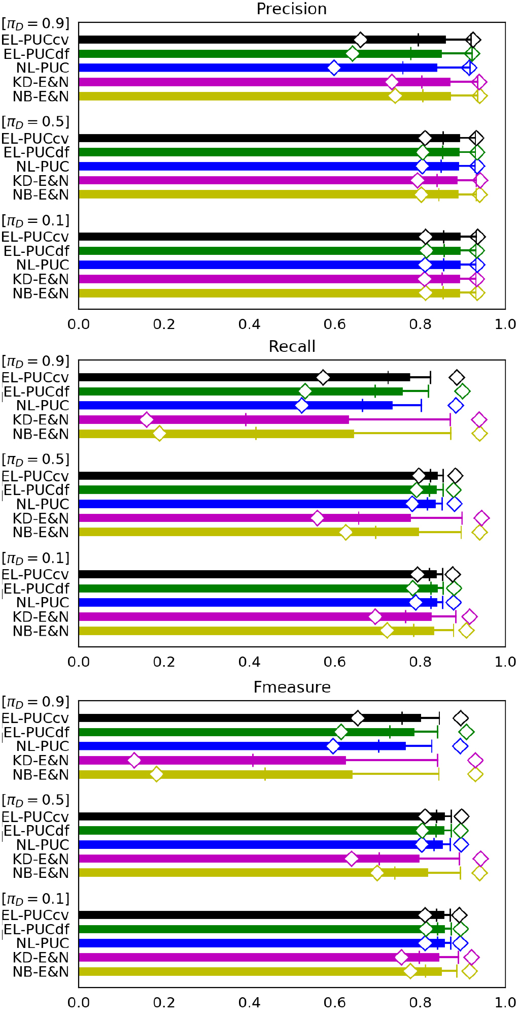
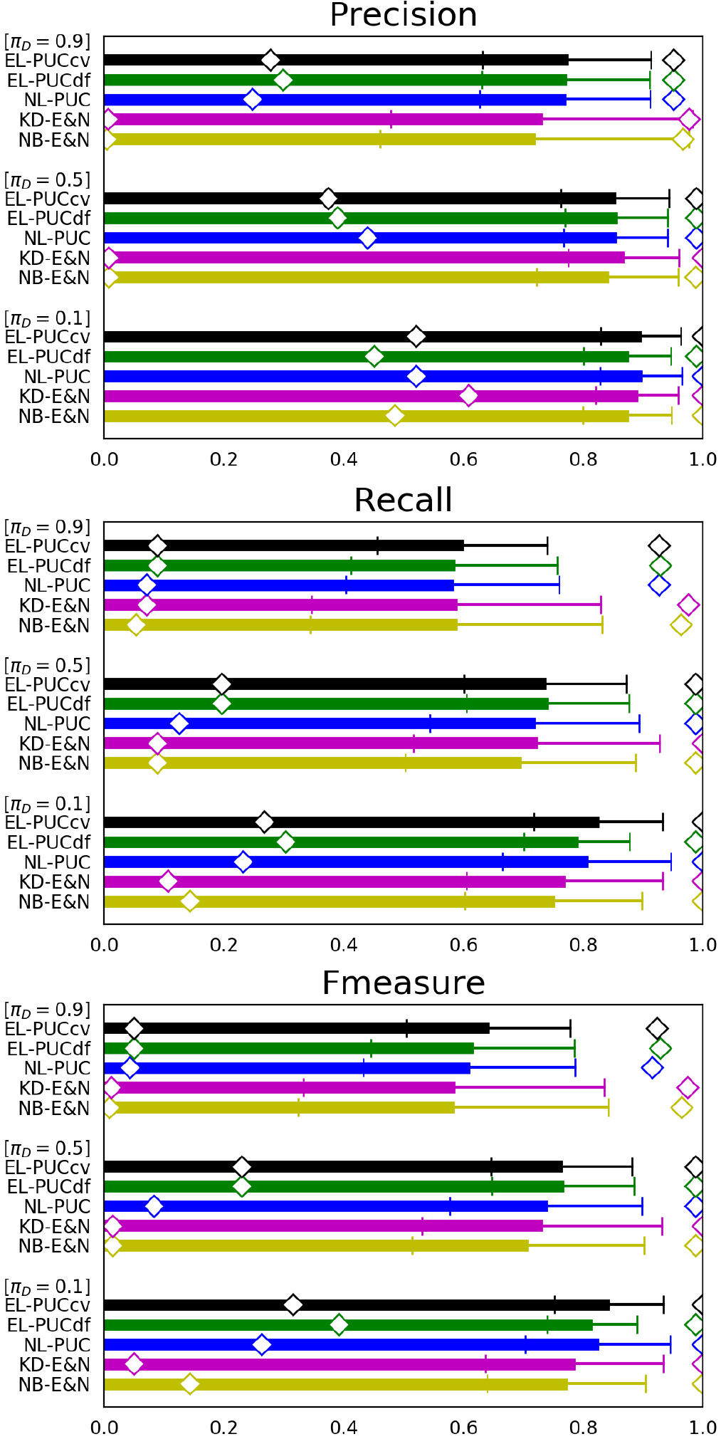
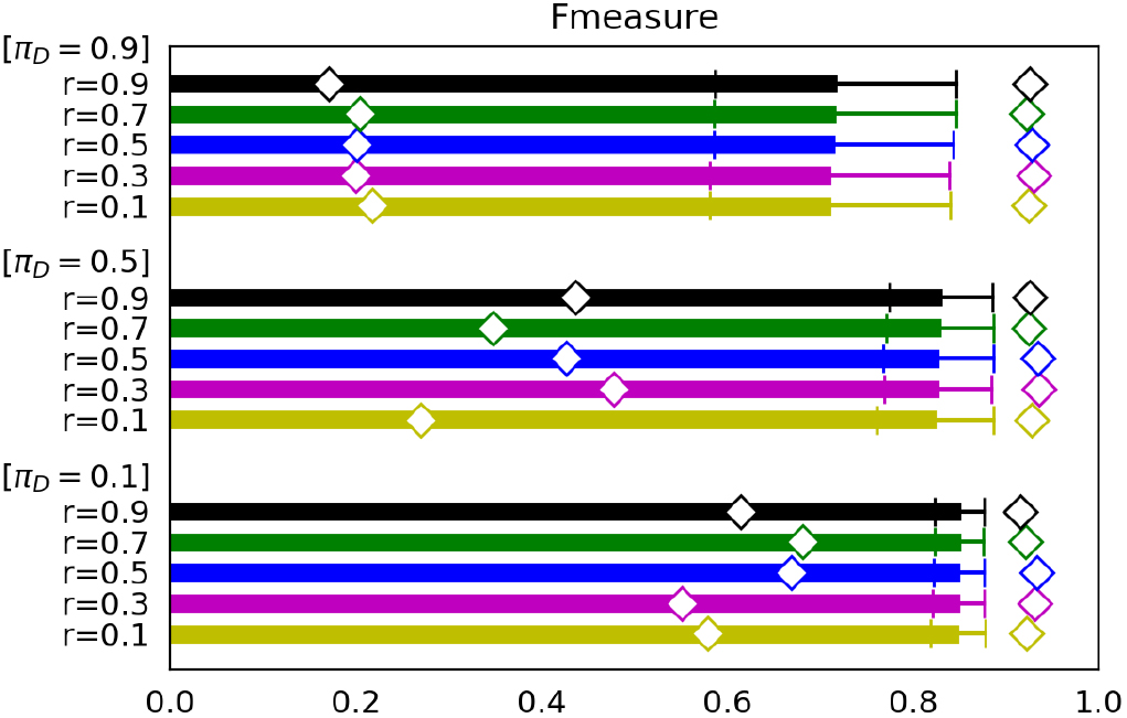
Performance for artificial data having three different 0.1, 0.5 and 0.9 ( 1000, 1000, 1000 and {0.1, 0.5, 0.9}).
Figure 1 shows comparisons of precision, recall and F-measure between the five PUCs in terms of the three class prior probabilities of : 0.1, 0.5 and 0.9. Under given with fixed data sizes 1000, 1000 and 1000, we generated 100 cases of for each class prior probability of : {0.1, 0.5, 0.9},i.e., 300 cases in total. The respective PUC trained using and is tested by using to measure its performance indecies in each case. A bar, a whisker and a diamond shape of a PUC in the figures represent the mean, the standard deviation and the minimum/maximum of the performance index over the 300 cases covering the three {0.1, 0.5, 0.9}, respectively. The mean represents the accuracy of a PUC over the difference of the class prior probabilities between and . The less standard deviation and the less interval between the minimum and the maximum show the higher robustness of a PUC to the difference.
In these figures, the accuracy and robustness of all PUCs mostly decrease with increasing , because the negative samples in become less while they are the unique information source on . NB-E&N and KD-E&N particularly lose their recall in this condition, since they use classifiers of labeled and unlabeled samples which do not capture the difference between the labeled positive samples and the unlabeled negative samples when almost all samples are positive. Nevertheless, all the three indecies show high accuracy and higher robustness of our three PUCs than NB-E&N and KD-E&N in almost all conditions. This comes from the fact that the classification measures Eqs (3) and (4) used in our PUCs are independent of the class prior probabilities. The accuracy of EL-PUCdf and EL-PUCcv is particularly higher than that of NL-PUC under 0.9. This may be because is kept small by estimating from both and , while is small as long as Assumption 2 holds on a continuous space [24, 10]. These effects make Eq. (2) in Theorem 2 to widely hold even under the large where the performance of NL-PUC is degraded by the shortage of the information on .
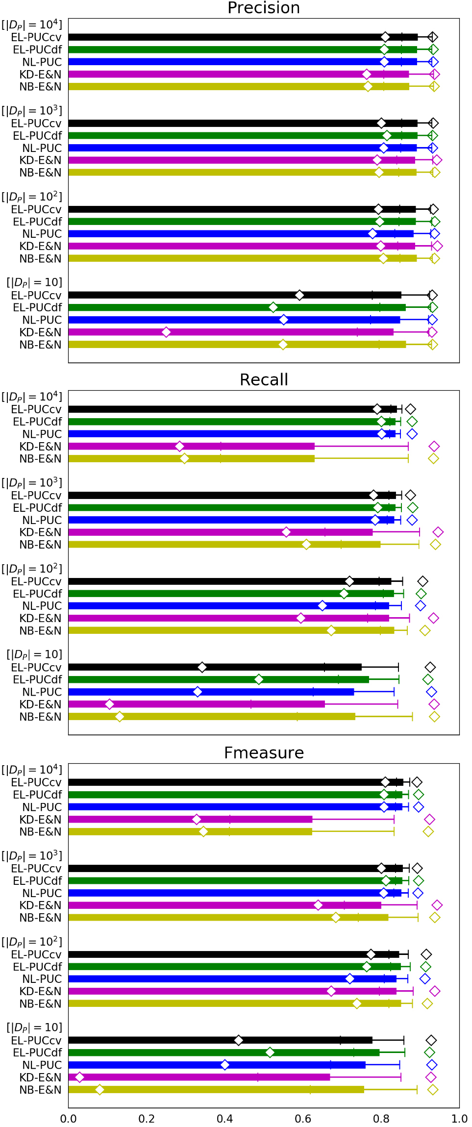
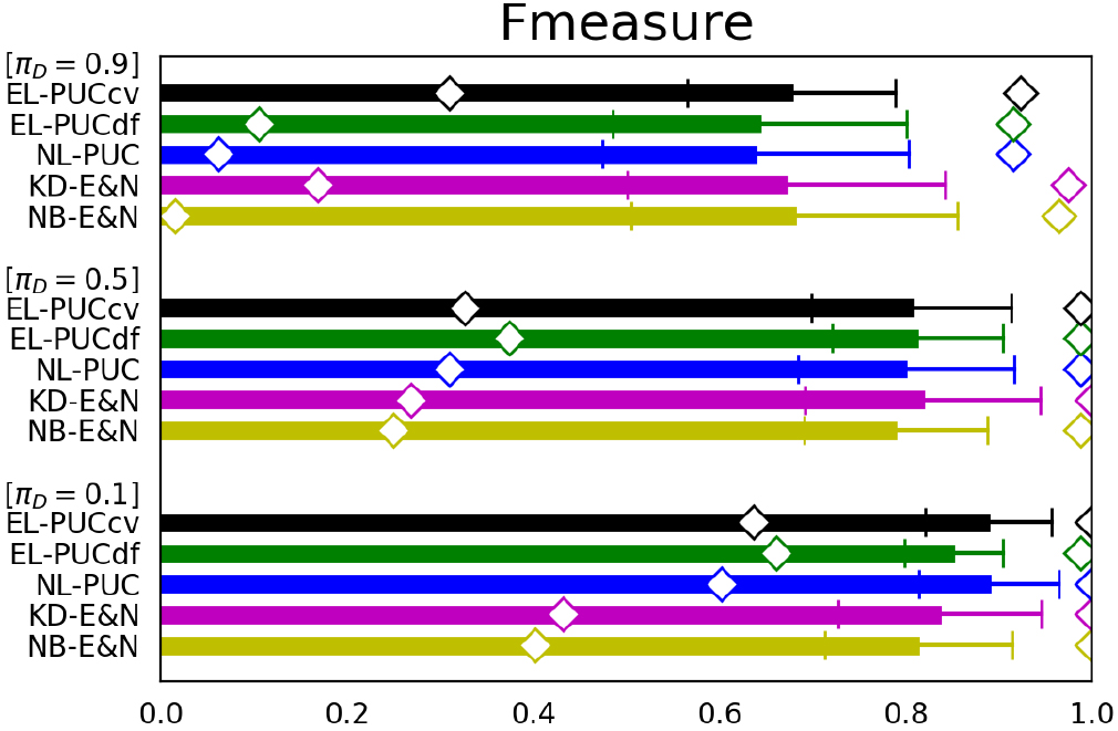
Performance for artificial data having various 10, 100, 1000 and 10000 ( 0.5, 1000, 1000 and {0.1, 0.5, 0.9}).
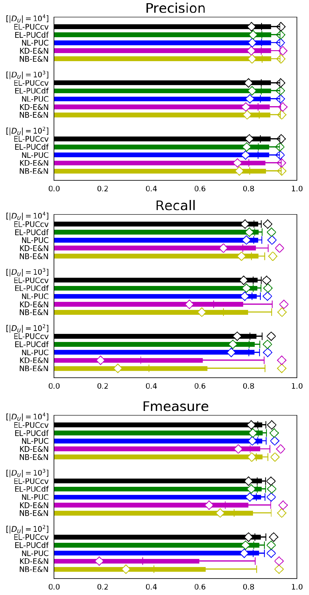
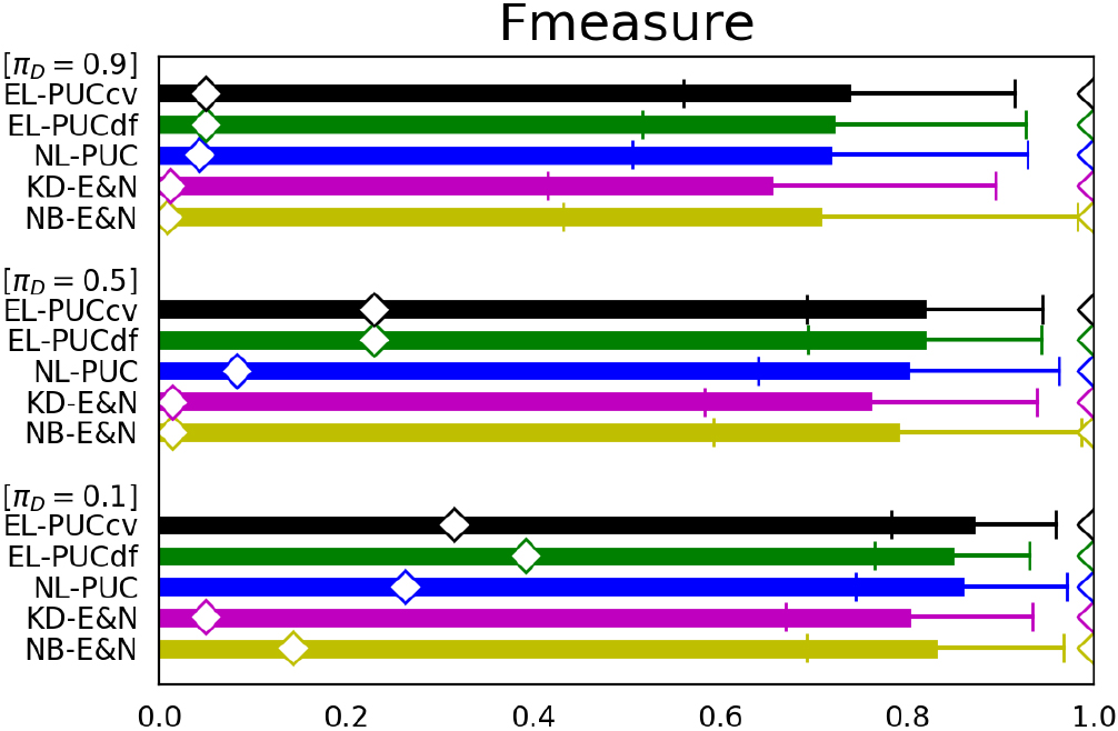
Performance for artificial data having various 100, 1000 and 10000 ( 0.5, 1000, 1000 and {0.1, 0.5, 0.9}).
Computation times of the five PUCs.
Figure 2 shows comparison of the three indices between the five PUCs over 10, 100, 1000 and 10000. As in Fig. 1, we generated 300 cases over 0.1, 0.5 and 0.9 under given , 1000 with fixed 0.5 and 1000 in an experiment, and measured the mean, the standard deviation and the minimum/maximum of the three indices of each PUC over the 300 cases covering the three {0.1, 0.5, 0.9}, respectively. Figure 3 was created for the comparison over 100, 1000 and 10000 under fixed 0.5, 1000 and 1000 in similar manner. In these figures, our three PUCs again show higher accuracy and robustness than NB-E&N and KD-E&N in the most conditions including the case of 10 in Fig. 2. Elkan & Noto’s PUCs show larger standard deviations and intervals between the minimum and the maximum of the accuracy. Particularly, they show significant decreases of the accuracy in the imbalanced conditions between and such as the cases of 10 and 10000 in Fig. 2, and 100 in Fig. 3. This is because they use classifiers of labeled and unlabeled samples which are statistically degraded under the highly imbalanced conditions. The accuracy of EL-PUCdf and EL-PUCcv is particularly higher than that of NL-PUC when a small size 10 and a large size 1000 are provided in Fig. 2. This character is consistent with the suggestion of Theorem 2 and (10) and (11).
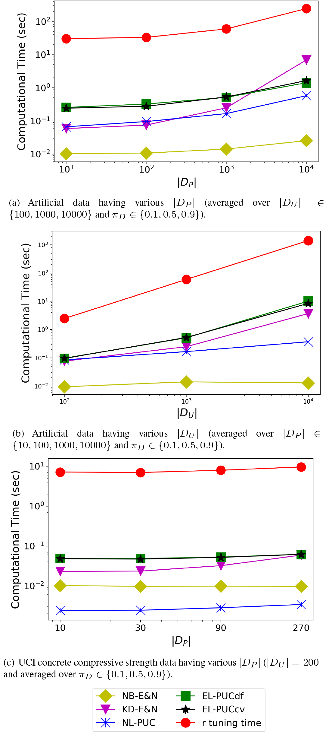
Figures 4a and b represent the dependency of the computation times required to train the five PUCs using the artificial data in log-log plots. The computation times under given were averaged over all combinations of and in the former, and those under given were averaged over all combinations of and in the latter. The line of “EL-PUCcv” shows its computation times after the tuning of the parameter , and the line of “r tuning time” indicates its times required for the tuning by the 10 fold cross validation. Since NL-PUC simply learns Eq. (4), its complexity for training is . Both EL-PUCdf and EL-PUCcv have their complexity of where is the number of the iteration of Eqs (4.2)–(7). In each iteration step, the computation of is repeated times in Eq. (6) where each is computed by Eqs (4.2) and (7) using samples. In the tuning, a test computes the pseudo F-measure using the samples proportional to where each sample is classified by using the other samples. This is repeated 10 times with the training of EL-PUCcv. Thus, the total complexity of the tuning is . NB-E&N and KD-E&N process samples for classifying a sample if it is labeled or unlabeled. They repeat this process times to evaluate the probability that a positive sample is labeled. Thus, their total complexity is . These facts are well reflected to Fig. 4a and b where the dependency of their computation times is linear or quadratic. Particularly, KD-E&N needs computation times comparable with or more than our proposed PUCs. Note that these computation times may be positively biased by some overhead process under small 10.
Performance for UCI concrete compressive strength data having various 0.1, 0.5 and 0.9 ( 200, {10, 30, 90, 270} and [0.1, 0.5, 0.9]).
Performance evaluation using UCI data
In the UCI repository, there are only a few data sets having known measurement processes. We used “Concrete Compressive Strength" (#samples: 1030, #observed variables [X]: 7, target variable [Y]: compressive strength), “Airfoil Self-Noise" (#samples: 1503, #observed variables [X]: 5, target variable [Y]: angle of attack), and “Steel Plates Faults" (#samples: 1941, #observed variables [X]: 26, target variable [Y]: sigmoid of areas) from the physical sciences. We removed their categorical variables, binarized the target variables by applying their median values as a threshold, and chose one of the binary values as positive. Thus, they became balanced data sets in terms of their positive and negative samples. In each data set, we drew 20% of the total to produce three having the probabilities 0.1, 0.5 and 0.9 to include positive samples, respectively. We also took extra 1%, 3%, 9% and 27% of the total to create four , respectively, by choosing positive samples only. Furthermore, we drew extra 10% of the total to produce three having 0.1, 0.5 and 0.9, respectively. For each of the three , we computed the mean, the standard deviation, and the minimum/maximum of the accuracy indices of the five PUCs by marginalizing over all combinations of and .
Figures 5–7 compare the results using these UCI data sets. Because the figures of precision and recall of the last two data sets show similar behaviors with those of the first one, they are omitted. The figures mostly show a similar tendency with those of the artificial data. Under the most conditions of , our three PUCs are more accurate and robust than NB-E&N and KD-E&N to the varieties of the size and the differences of the class prior . Though the difference between our three PUCs are not very significant, EL-PUCcv provides the top average accuracy in many cases.
Figure 4c indicates the computation times to train the five PUCs using Concrete Compressive Strength data set. Because the size of the data set is small, the computation times of their overhead processes became dominant. Nevertheless, NL-PUC having lower complexity in essence was faster than NB-E&N, because the load of the kernel density based estimation was not significant for the small data set. We observed similar behaviors for the other two data sets.
Performance for UCI airfoil self-noise data having various ( 300, {15, 45, 135, 405} and [0.1, 0.5, 0.9]).
Performance for UCI steel plates faults data having various ( 400, {20, 60, 180, 540} and [0.1, 0.5, 0.9]).
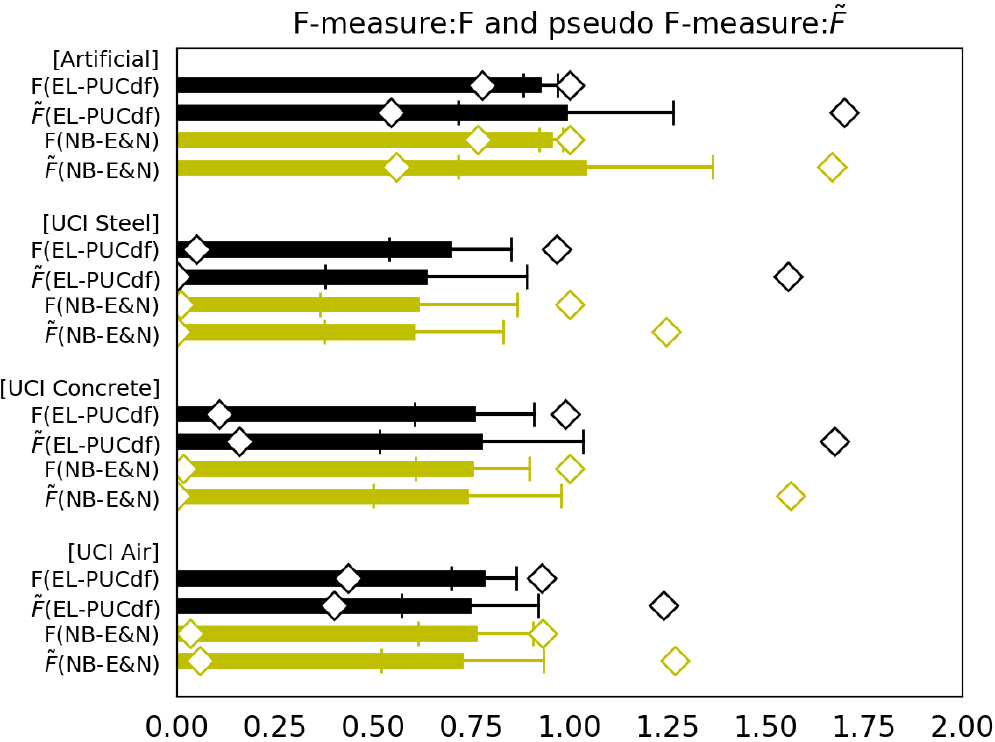
Comparison between F-measure: and pseudo F-measure: of EL-PUCdf and NB-E&N for various data ( 10, 1000 and {0.1, 0.5, 0.9} for artificial data, and the conditions of Fig. 5–7 for UCI data).
Discussion
All results in Section 5 indicate that EL-PUCcv, which tunes by using the pseudo F-measure: , achieves the highest or comparable accuracy and robustness among our three PUCs. This reflects Lemma 4 that we can appropriately tune the parameters of the classifiers by using . The traditional F-measure: and of EL-PUCdf depicted in Fig, 8 more directly represents their consistency. Note that can be larger than unity according to its definition in Lemma 4. Though the standard deviations and the intervals between the minimum and the maximum of are larger than those of , i.e., is less robust to the deviations of from under various conditions, the means of and show consistent behaviors over the four data sets. This supports the use of to evaluate the accuracy of our likelihood based PUCs. Figure 8 also shows the comparisons of and for NB-E&N which uses the aforementioned one sample setting. Although this setting does not match with the assumptions required to the consistency of , and of NB-E&N indicates their consistency comparable to those of EL-PUCcv. This may be because the probability to correctly classify a positive sample as positive by the Gaussian Naïve Bayes classifier used in NB-E&N is moderatly affected by the variation of the class priors . This shows that the pseudo F-measure is widely applicable to qualitatively assess the performance of the PUCs.
Dependency of EL-PUC on parameter for artificial data having various ( {15, 45, 135, 405}, {100, 1000, 10000} and [0.1, 0.5, 0.9]).
According to the dependency of EL-PUC’s accuracy on the parameter as indicated by the lemmas and the theorems in Subsection 4.3, we proposed EL-PUCcv which selects an optimal using the cross validation to achieve the highest accuracy. Meanwhile, Fig. 9 shows F-measure of EL-PUC over various for the artificial data having three 0.1, 0.5 and 0.9 where all other conditions were marginalized. In the marginalized view, the accuracy of EL-PUC does not have any clear dependency on . This supports the experimental results in Section 5 indicating the small differences of the accuracy and the robustness between EL-PUCdf and EL-PUCcv in most cases. On the other hand, EL-PUCcv requires extremely large computation times for the parameter tuning as shown in Section 5. These facts suggest the limited applicability of EL-PUCcv to practical measurement tasks particularly when the available time for training is limited.
Besides, EL-PUCdf shows higher accuracy and robustness than NL-PUC under large and small while the computation time of EL-PUCdf is larger than that of NL-PUC. Therefore, we need to consider the trade-off between the classification performance and the computation time for the selection of the two approaches.
Real-world application
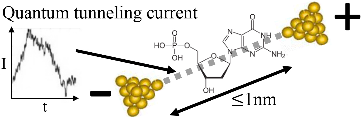
We applied our PUCs to noise reduction in a real-world single molecule measurement [25]. Figure 10 depicts the core part of the sensor called a “nano-gap.” The passage of an object between two nanoscopic electrodes is observed as an electric pulse induced by the quantum tunneling effect. Our task is to classify each pulse into a target molecule and a contaminant in the solvent based on the pulse outline in real time. A technical difficulty here is that the solvent containing no contaminants is hardly produced. Therefore, we always obtain a data set containing the target molecule’s pulses with the contaminant’s noise pulses, whereas we can get a data set containing the noise pulses of the contaminants only by observing the solvent without the target molecules. Moreover, the nano-gap sensor is disposable in every measurement task. Because characters of the nano-gaps are mutually different depending on the fluctuations of their manufacturing processes while a nano-gap is stable during a measurement task, we need to train the classifier in a short on-line period for the quick start at the beginning of every measurement task. Accordingly, the time for acquiring the noise pulses is very limited, while the target pulses with the noise pulses are acquired for a long period in their measurement. These required specifications meet with the conditions addressed by our proposed PUCs.
Performance comparison of noise reduction
Time for
Method
Training
NB-E&N
1.47 msec
0.572
0.582
0.592
KD-E&N
4.90 msec
0.318
0.322
0.282
NL-PUC
7.29 msec
0.715
0.671
0.652
EL-PUCdf
736.19 msec
A Single molecule sensor.
In our application, a pulse signal time series between the start and the end of the pulse is partitioned into 10 equi-width time intervals, and the signal points in each interval are averaged. The pulse outline is a 10 dimensional vector consisting of the 10 averages. We acquired consisting of the noise pulse outlines, which were labeled as positive, in a short initial on-line period for the quick start. Successively, the unlabeled pulse outlines of the target molecules with the contaminants are acquired for a certain limited period to create where their labels are estimated by a PUC during its training and the pulses classified into the target molecules become the initial part of the measurement output. After the PUC is trained by using and , the on-line noise reduction of new incoming pulses starts. The ratio of the targets and the contaminants in the solvent, i.e., the class prior, rapidly varies in the on-line measurement.
We used the pseudo F-measure to evaluate the performance of the noise reduction, because the ground truth of the classification was unknown. We acquired an extra labeled positive test set together with in the initial short period, and further acquired some unlabeled test sets for computing of the five PUCs after the on-line measurement started. Their sizes were defined as 20, 800 and 100 by following the aforementioned specifications and the convenience to compute .
Table 1 shows the performances of the four PUCs applied to three . We excluded EL-PUCcv because its large computation time is not suitable for on-line processing. The same codes and the same PC with Section 5 were used. The class prior of the first acquired immediately after the start of the on-line measurement is almost same with . Then, contaminants in the solvent rapidly increased over the periods acquiring the second and third which made the second as and the third as . Note that is not normalized into [0,1], and its value does not represent the absolute accuracy, while the larger show a better performance. The best numbers are underlined in each column. Particularly, EL-PUCdf showed the best , while it takes relatively large computation time for its training. NL-PUC is better for the instant start of the on-line measurement, and EL-PUCdf is better if the dead time for nearly 1sec is allowed. The entire performance of NB-E&N and KD-E&N were significantly worse than those of NL-PUC and EL-PUCdf becuase of the small 20 available for the training. This is consistent with the result for the artificial data depicted in Fig. 2.
Conclusion
Our proposed PUCs show high accuracy and robustness under wide conditions. They are particularly advantageous when the numbers of the labeled positive samples and the unlabeled samples are imbalanced and when the positive class prior probability is dominant. Moreover, our proposed EL-PUC provides better accuracy than our proposed simple NL-PUC when the number of the labeled positive samples is limited and when the positive class prior probability is dominant, while EL-PUC needs more computation time.
In various practical problems, the labeled positive dataset may be contaminated by the falsely labeled negative instances. Some instances in and may have missing values. The PUCs including our proposed approaches and the past approaches are not applicable to such incomplete datasets. These issues remain for future work. Moreover, we proposed our PUCs using the nonparametric estimation. The idea may be extended to discriminative frameworks.
References
1.
BengioY.DelalleauO. and RouxN.L., Efficient non-parametric function induction in semi-supervised learning, in Proc. AISTATS05: the 10th International Workshop on Artificial Intelligence and Statistics, 2005, pp. 96–103.
2.
BlanchardG.LeeG. and ScottC., Semi-supervised novelty detection, J. Machine Learning Research11 (2010), 2973–3009.
3.
CalvoB.InzaI.LarranagaP. and LozanoJ.A., Wrapper positive bayesian network classifiers, Knowledge and Information Systems33 (2010), 631–654.
4.
du PlessisM.C.NiuG. and SugiyamaM., Class-prior estimation for learning from positive and unlabeled data, in Proc. ACML15: the 7th Asian Conf. on Machine Learning, vol. 45, 2015, pp. 221–236.
5.
du PlessisM.C. and SugiyamaM., Semi-supervised learning of class balance under class-prior change by distribution matching, Neural Networks50 (2014), 110–119.
6.
du PlessissM.C.NiuG. and SugiyamaM., Analysis of learning from positive and unlabeled data, in Proc. NIPS14: Advances in Neural Information Processing Systems, vol. 27, 2014, pp. 703–711.
7.
ElkanC. and NotoK., Learning classifiers from only positive and unlabeled data, in Proc. KDD08: the 14th ACM SIGKDD Int. Conf. on Knowledge Discovery and Data Mining, 2008, pp. 213–220.
8.
GamaJ.Žliobait eI.BifetA.PechenizkiyM. and BouchachiaA., A survey on concept drift adaptation, ACM Computing Surveys (CSUR)46 (2014), 44:1–44:37.
9.
HajizadehS.LiZ.DollevoetR.P.B.J. and TaxD.M.J., Evaluating classification performance with only positive and unlabeled samples, in Proc. S+SSPR14: Structural, Syntactic, and Statistical Pattern Recognition, vol. LNCS 8621, 2014, pp. 233–242.
10.
HengartnerN.W. and Matzner-LoberE., Asymptotic unbiased density estimators, ESAIM: Probability and Statistics13 (2009), 1–14.
11.
JainS.WhiteM. and RadivojacP., Recovering true classifier performance in positive-unlabeled learning, in Proc. AAAI17: the 31st AAAI Conf. on Artificial Intelligence, 2017, p. 3060.
12.
KomlosK.PopovicsS.NurnbergerovaT.BabalB. and PopovicsJ.S., Ultrasonic pulse velocity test of concrete properties as specified in various standards, Cement and Concrete Composites18 (1996), 357–364.
13.
LeeW.S. and LiuB., Learning with positive and unlabeled examples using weighted logistic regression, in Proc. ICML03: the 20th Int. Conf. on Machine Learning, 2003.
14.
LewisA., Getdist: Kernel density estimation, github: getdist document, University of Sussex, 2015. http://cosmologist.info/notes/GetDist.pdf.
15.
LiX.-L.YuP.S.LiuB. and NgS.-K., Positive unlabeled learning for data stream classification, in Proc. SDM09: the 2009 SIAM Int. Conf. on Data Mining, 2009, pp. 259–270.
16.
Marina De MarcoE.A., Influence of left ventricular stroke volume on incident heart failure in a population with preserved ejection fraction (from the strong heart study), American Journal of Cardiology119 (2017), 1047–1052.
17.
MenonA.RooyenB.V.OngC.S. and WilliamsonB., Learning from corrupted binary labels via class-probability estimation, in Proc. ICML15: the 32nd Int. Conf. on Machine Learning, vol. 37, 2015, 125–134.
18.
NiuG.du PlessisM.C.SakaiT.MaY. and SugiyamaM., Theoretical comparisons of positive-unlabeled learning against positive-negative learning, in Proc. NIPS16: Advances in Neural Information Processing Systems, Vol. 29, 2016, pp. 1199–1207.
19.
PanS.J. and YangQ., A survey on transfer learning, IEEE Trans. on Knowledge and Data Engineering22 (2010), 1345–1359.
20.
PfeffermannD.SkinnerC.HolmesD.J.GoldsteinH. and RasbashJ., Weighting for unequal selection probabilities in multilevel models, J. the Royal Statistical Society. Series B (Statistical Methodology)60 (1998), 23–40.
21.
RamaswamyH.G.ScottC. and TewariA., Mixture proportion estimation via kernel embedding of distributions, in Proc. ICML16: the 33rd Int. Conf. on Machine Learning, vol. 5, 2016, pp. 2996–3004.
22.
SaerensM.LatinneP. and DecaesteckerC., Adjusting the outputs of a classifier to new a priori probabilities: A simple procedure, Neural Computation14 (2002), 21–41.
23.
ScottC., A rate of convergence for mixture proportion estimation, with application to learning from noisy labels, in Proc. AISTATS15: the 18th Int. Conf. on Artificial Intelligence and Statistics, vol. 38, 2015, pp. 838–846.
24.
SilvermanB.W., Density Estimation for Statistics and Data Analysis, Chapman & Hall/CRC, 1985, ch. 3.3 and 43.
25.
TsutsuiM.TaniguchiM.YokotaK. and KawaiT., Identifying single nucleotides by tunneling current, Nature Nanotechnology5 (2010), 286–290.
26.
WangB. and WangX., Bandwidth selection for weighted kernel density estimation, Electronic J. of Statistics (2007). doi: 10.1214/154957804100000000.
27.
WardG.HastieT.BarryS.ElithJ. and LeathwickJ.R., Presence-only data and the em algorithm, Biometrics65 (2009), 554–563.
28.
WashioT.ImamuraG. and YoshikawaG., Machine learning independent of population distributions for measurement, in Proc. DSAA17: the 4th IEEE Int. Conf. on Data Science and Advanced Analytics, 2017, pp. 212–221.
29.
ZhuX.GhahramaniZ. and LafferJ., Semisupervised learning using gaussian elds and harmonic functions, in Proc. ICML03: the 20th Int. Conf. on Machine Learning, 2003.