
Abstract
This paper presents an Automatic Parking Space Detection (APSD) algorithm designed to reduce traffic in cities while offering an information system of available parking zones. The main aim of such a system lies in its ability to identify parking spaces in a distributed manner, achieved by installing multiple APSD systems across a fleet of vehicles. This fleet, during its regular operations, communicates the availability of parking spaces to a centralized information system. Our methodology employs a rule-based system that seamlessly integrates a variety of neural networks for different specific tasks. These tasks include depth estimation, road segmentation, and vehicle detection. This approach would fall into a modular category instead of an end-to-end solution, using the Málaga Urban Dataset in the experiments. We present a preliminary experiment for parameter settings and an ablation study to quantify each subsystem contribution to the results. The proposed system achieves a parking space detection F1 score of 0.726.
Keywords
Introduction
Traffic control plays a central role in sustainability policies in cities [1, 2, 3]. One of the main aspects that influences traffic conditions is the management of available parking spaces, as drivers waste a lot of time looking for a parking spot [8], hindering traffic flow. Urban smart parking is a new and wide concept that aggregates different applications related to vehicle parking in cities, including private parking management, parking payment, guidance to the nearest parking space or detection of available parking spaces.
The autonomous vehicle (AV) paradigm shift faces new challenges, like intersection management [4, 5], vehicle to vehicle (V2V) or vehicle to infrastructure (V2I) communication [6, 7], lane assistant or the autonomous vehicle maneuvering parking (ego-vehicle parking), among others.
The Automatic Parking Space Detection (APSD) problem can be faced using different strategies, sensors or environmental conditions depending on whether the parking spot is detected for. APSD systems for the ego-vehicle parking problem are usually mounted on-board. On the contrary, the APSD systems oriented to share the availability of parking spaces to other drivers are usually part of the infrastructure in very controlled environments, like parking lots. Our proposal hybridizes previous approaches in the sense that we employ an on-board APSD system to share information of the available parking spots in uncontrolled environments.
Diagram of the proposed automatic parking space detection (APSD) system. The system is composed by two blocks. The calibration block is only performed once at system initialization, while the detection is performed at each frame. The output of the system is the bounding box of every detection in the current location.
Restricting to visual sensors, previous works mostly focus on the estimation of parking spaces by detecting painted marks on the floor that delimit each parking spot [9, 10, 11, 12, 13, 14, 15, 16, 17]. The detection of parking lines can be addressed using both classical methods [18, 19, 20] and neural networks [21, 22, 23]. These methods are usually explored in highly controlled scenarios.
Other approaches create a 3D reconstruction of the environment [26, 27, 28]. These works detect parking spaces determining the presence of delimiting elements in the scene such as cars, pillars, etc.
Most of the ego-vehicle parking works use a bird’s eye strategy creating a 360∘ reconstruction [29, 30, 31, 32]. For this reason, a large majority of benchmark datasets use this type of imagery. The ps2.0 dataset (Parking Slot dataset), consists of 9827 training images and 2338 test images [33]. The dataset is formed by surround-view images synthesized from four fisheye cameras. Another dataset is the PSV (Panoramic Surround-View dataset) [34] that provides 4200 surround-view (360 degrees around the vehicle) labeled images. Labels include parking slots and different line classes (solid white lines, white dashed lines, yellow solid lines and yellow dashed lines).
As stated before, there are other approaches aimed to share the availability of parking spaces that combine prior knowledge of the parking capacity and car detection to estimate free parking space in highly controlled environments [24, 25]. These systems work by counting the number of empty spaces available, usually without localizing them and using some kind of urban infrastructure, like ultrasonic sensors, outdoor displays, etc.
Visual parking space detection in uncontrolled and outdoor environments is a hard and open problem. On the one hand, it involves the detection of an empty space in an image that, in general, contains objects from the background such as sidewalks, floor, buildings facades, etc. As a consequence, a parking space can not be characterized by a set of visual features in every possible situation. This makes them difficult to detect for expert systems or machine-learning-based methods. On the other hand, parking space configuration can be organized at an angle, parallel or perpendicular fashion, which also affects the detection of relevant visual features to characterize them. In addition, parking spaces are sometimes delimited by markers and sometimes not, or these markers can be occluded by vehicles. Finally, the task of distinguishing between moving and parked vehicles in the scene is needed when vehicle detections are used for the parking space estimation.
Calibration stage. (a) Example of RGB input calibration image, (b) depth map and (c) road segmentation map.
In this work, we propose a computer vision system to detect parallel parking spaces by combining machine learning methods. In particular, we propose the use of neural networks for the visual detection and semantic segmentation, and a geometric rule-based system that uses the information provided by those networks to make a decision about the presence of a free parking space.
As most on-board automatic parking space detection systems are aimed to help the driver to park its own vehicle or even to create an autonomous park assistant, APSD systems usually need for a surround-view image built from several cameras (usually four: frontal, rear and two more under the side mirrors). With those views, the system would detect the road marking paints in order to guide the driver or the autonomous park assist software during the maneuvering. However, our proposed system is oriented to detect parking gaps while normal operation for creating a distributed service of available parking spaces. Thus a single front camera and an on-board computing device should be enough for this purpose.
From a software perspective, our parking space detection system is composed of specialized modules. Figure 1 shows a visual overview representation of the system. It is divided into two main parts: (i) an off-line calibration phase that is executed only once, and (ii) an on-line free parking space detection module that is executed on each captured frame.
The calibration phase receives a single RGB image as input and estimates, (i) a depth map and (ii) a semantic segmentation map (see Fig. 2).
The detection module uses (i) a city model that stores the information about the parking zones distribution in the city, (ii) a distance function as depth estimation lookup table in the ground plane, (iii) the side road limits and (iv) the vanishing point coordinates calculated during the calibration. This module receives a single image as input at every time step to search for parking spaces.
To generate depth maps, perform object segmentation, and vehicle detection, we employed general-available networks without an specific training for our problem and the dataset.
Calibration module
The calibration module is executed once at the beginning of the process. In this module, we model the 2D depth map as a function that estimates the distance at which a vehicle detection is located, based only on its vertical coordinate. In addition, the vanishing point coordinates as well as the road border line functions are estimated. In this way, without any homography-based calibration, we guarantee the compatibility of the algorithm with non-specialised and uncalibrated hardware.
Vehicle depth estimation involves generating a ground plane depth map (a). In this process, depth values from the central region are extended to both sides of the road. Subsequently, the depth data is modeled using polynomial functions of varying degrees. (b) The original data is denoted by a dotted blue line, the second-degree polynomial function by a green dashed line, the third-degree polynomial function by a red solid line, and the fourth-degree polynomial function by a pink dashed line.
The depth image is obtained using the Monodepth2 depth estimation network [35]. Among the different variations of the architecture provided by the authors, the mono+stereo version, with an output resolution of 640
Road segmentation
In this module, a segmentation of the roadway is performed using the Pyramid Scene Parsing Network (PSPNet) architecture [36]. In order to select the segmentation network, a performance study of several architectures was made in [40]. The PSPNet architecture consists of a feature extractor followed by a pyramid parsing module to obtain the representation of the different subregions. We use a Residual Network with 50 layers (ResNet50) module as a feature extractor [37]. Then, an upsampling and concatenation of the layers obtained in the previous stages is applied to obtain the complete feature representation. Finally, this feature map is fed into a convolutional layer and the final prediction per-pixel is obtained. We apply this model in our problem to obtain a 1024
This module has been trained for 100 epochs with a subset of the Cityscapes [38] data set using the fine annotations. This dataset has 2975 training images, 500 validation images and 1525 test images.
Performance comparison of state of the art detection networks in vehicle detection
Performance comparison of state of the art detection networks in vehicle detection
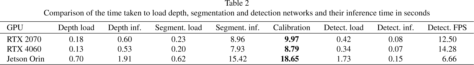
Comparison of the time taken to load depth, segmentation and detection networks and their inference time in seconds
The estimation of the distance among vehicles in the scene is a hard problem and it is a key step for the overall system accuracy. Vehicle detections in the image exhibit not one, but a set of different depth values, due to their orientation with respect to the camera. In addition, inside the bounding box of each detection, parts of other vehicles, road, or other objects may appear. Also, the obtained accuracy at further distances than 30 meters is not enough to distinguish parking spaces properly. Moreover, the execution of the depth estimation network at each frame is computationally expensive.
Thus, instead of having a running monocular depth estimation network on every frame, we estimate the distance from the vehicles to the viewer using a function that relates the depth of every pixel with its vertical coordinate. This function accurately approximates the distance on the ground plane. The data needed to calculate such a distance function are the depth map of a representative image of the scenario and its road segmentation map, that acts as a mask of the ground plane (see Fig. 3a). The vertical coordinates of the road pixels are associated with the depth mean value of the central region of their row (red vertical region in Fig. 3a). Then, these discrete depth data along the y-axis are adjusted to a fourth order polynomial function. The depth of a vehicle is set as the value of this function at the vertical coordinate of the vehicle’s ROI lower corner.
Figure 3b shows different distance estimation functions for this data. Note that lower pixels in the image (corresponding to large y-coordinates from the upper-left corner) result in near distances. The original data is denoted by a dotted blue line, the second-degree polynomial function by a green dashed line, the third-degree polynomial function by a red solid line, and the fourth-degree polynomial function by a pink dashed line.
Vanishing point estimation
In this phase we get the scene vanishing point and the road border lines using the road segmentation mask.
The vertical coordinate of the vanishing point is set as the index of row
Detection module
This stage is devoted to the detection of parking spaces from the vehicles in the scene. It is iteratively executed at run time on those city zones where parking is allowed. This system is composed of a set of subsystems that are detailed in the next subsections.
Modeling
This module activates the parking space detector when the system is acquiring images in a city area where parking is allowed. The modeling of the environment can be done using GPS information. We can process driving routes and mark the start and end of areas where parallel parking is allowed, differentiating between the right and left side of the road, to create the model. Crosswalks or driveways can be marked to avoid considering them as parking spaces. So, the following detection stages only run when the on-board system is in an area where parking is allowed.
Vehicle detection
Example of vanishing point estimation. The orange striped line marks the right side of the road and the blue dotted line marks the left side. The vanishing point is represented by a green triangle.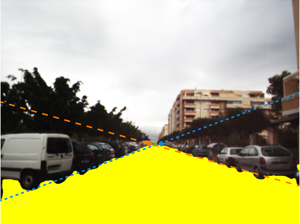
The core of the method is a vehicle detection network. To select the detection neural network, we test different state-of-the-art detection networks available in the Tensorflow ModelZoo library, all of them trained with COCO dataset, [39] on a subset of 500 images from the Cityscapes dataset. Models are compared using standard metrics: accuracy, recall, F1 score and running time. We consider that a correct detection is produced when a IoU of 0.5 between prediction and ground truth is met.
Examples of labeled frames from the malaga urban dataset. The groundtruth labels are shown as red boxes.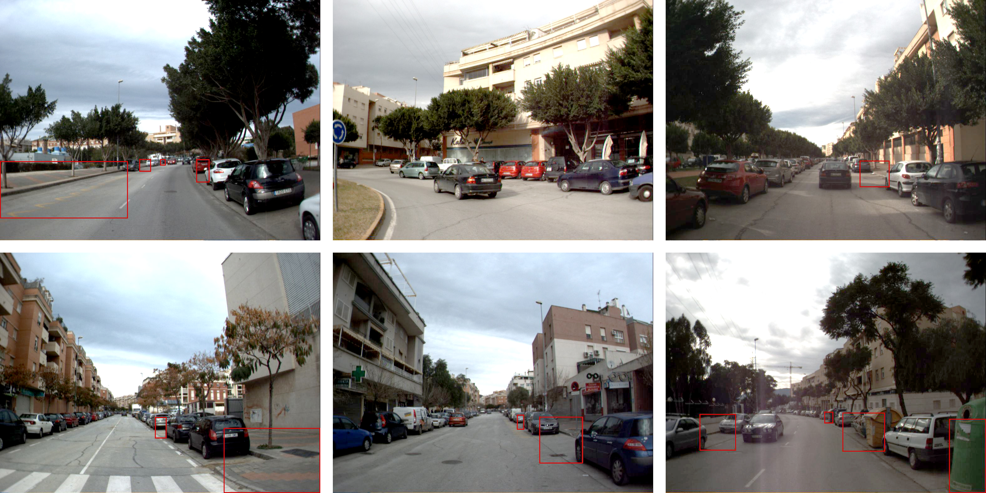
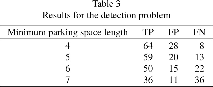
Results for the detection problem
Results for the classification problem
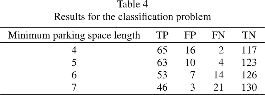
Table 1 shows the obtained results for 7 different detection networks. As it can be observed, EfficientDet obtains the best precision results while SSD-Mobilenet is the less consuming alternative in terms of time and memory. A more in-depth study of different detection network architectures (in particular Faster RCNN, SSD Mobilenet, YOLO-v5n, YOLO-v5n6, YOLO-v5-S, YOLO-v8-N, SSD Mobilenet v1, SSD Mobilenet v2 and SSD Inception v2) is detailed in [40]. Taking into consideration a compromise between quality and performance metrics, we choose Faster-RCNN ResNet for vehicle detection.
This stage is dedicated to distinguish between parked and moving vehicles, in order to identify parking spaces correctly. To achieve this, the position of the bounding box detection center is compared to the road border lines. A vehicle detection is removed when the center of its bounding box is located within the road borders.
As result we obtain two sets of vehicle positions, one with the positions of the vehicles parked on the right side of the road and other with those on the left side.
Maximum depth for analysis
Depth estimation at far distances has low accuracy and causes problems in the detection of distant parking spaces. For this reason, a detection limit has been set to discard vehicle detections at long distances. We have considered two distance thresholds: 20 and 30 distance units. As explained is Section 2.1.3 above, the depth of the vehicles is set to the resulting value of the distance function at the vertical coordinate of the base of their bounding box.
Parking space detection
Finally, the system computes the distance between any pair of consecutive vehicles in order to take a decision. A free parking space is reported when such a distance is large enough to place a vehicle on this space.
Moreover, as the first and last vehicle detection may leave a gap at the front or at the end, we check whether there is sufficient distance between the nearest vehicle and the visible limit of the parking area, and between the farthest vehicle and the detection limit, respectively.
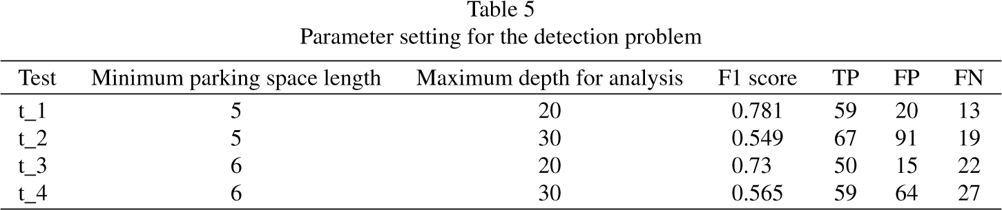
Parameter setting for the detection problem
Parameter setting for the detection problem
Results obtained in datasets A and B using the combination parameters with the best results in parameter setting: (a) detection problem, (b) classification problem.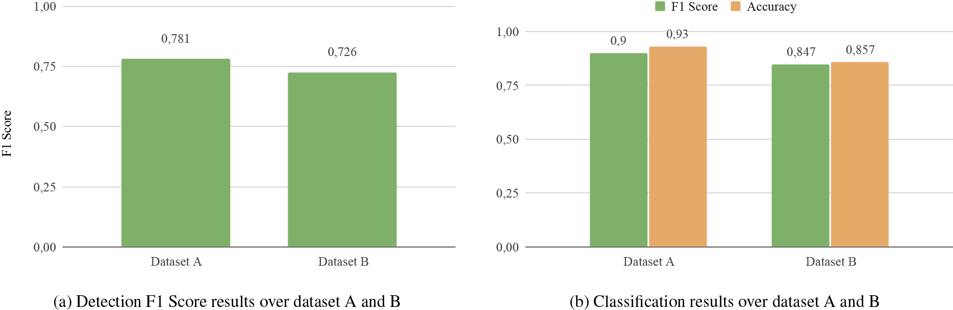
The output of the module is a vector with the final parking spaces locations.
In this section we present the results obtained from our experimental design. First we offer a description of the dataset used in our experimental setup. We also report the results obtained from a preliminary experimentation oriented to set model parameter values. The next section presents and discusses the results obtained. Finally, an exhaustive ablation study is performed to identify the contribution of each part of the proposed model.
We consider the problem of free parking space detection from two perspectives: classification and detection. The former consists of determining if there is any free parking space or not at a given frame. The latter tries to locate each free parking space in the image.
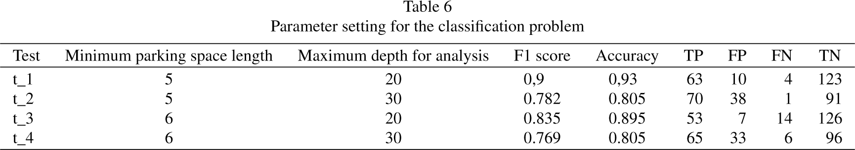
Parameter setting for the classification problem
Parameter setting for the classification problem
Results obtained in the ablation study on the data B. Figure 7a shows the results obtained in the different variations of the system in terms of F1 Score understanding the problem as a detection problem and image 7c shows its number of true positives, false positives and false negatives. Image 7c and 7d show the results obtained in the different variables of the system understanding the problem as a classification problem. Figure 7c shows the results in terms of F1 Score and Accuracy, while Fig. 7d shows the results in terms of true positives, false positives, false negatives and true negatives.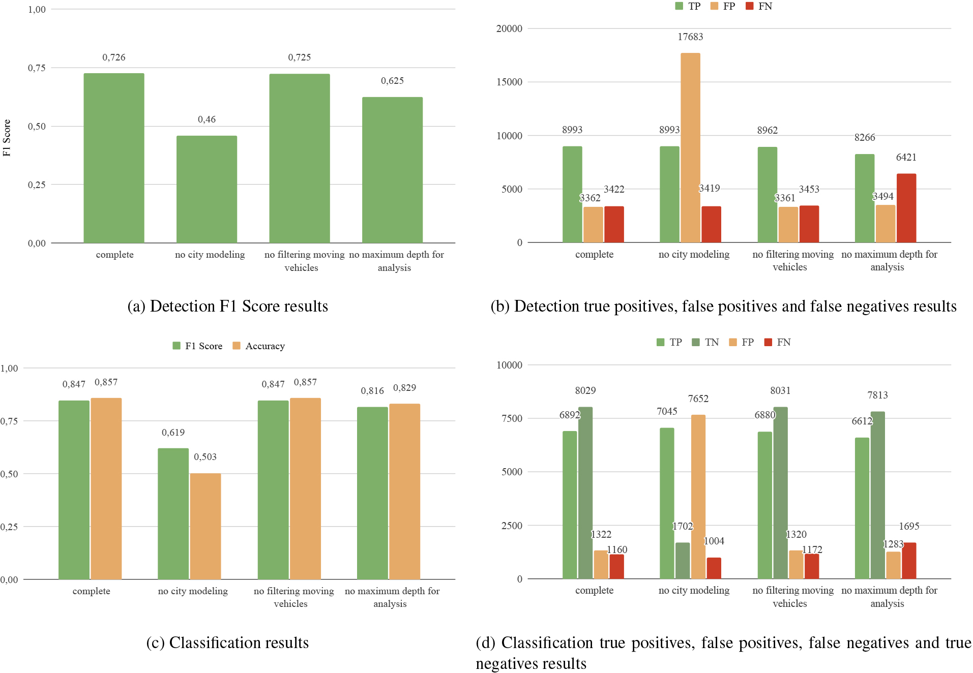
Experiments were conducted using three different platforms: a desktop consumer platform, a laptop platform and an embedded platform.
The desktop platform consists of an Intel Core i7-8700, 3.2 GHz, 32 GB RAM equipped with an NVIDIA RTX 2070 GPU with 8 GB GDDR graphics memory.
The laptop platform is based on a 2022 Intel i5-12450H, 2.0 GHz, 16 GB RAM with an NVIDIA RTX 4060 GPU with 8 GB GDDR graphics memory.
The embedded platform is an NVIDIA AGX Orin with a 12-core Arm Cortex-A78AE v8.2 64-bit CPU, 1.3 GHz with 64 GB RAM, 3 MB L2 and 6 MB L3 cache with a 2048-core NVIDIA Ampere architecture GPU including 64 Tensor Cores. This platform is especially suited for automotive applications with variable power consumption of 15–60W.
Table 2 shows the time used by these platforms for the loading and inference of the depth estimation, road segmentation and vehicle detection networks.
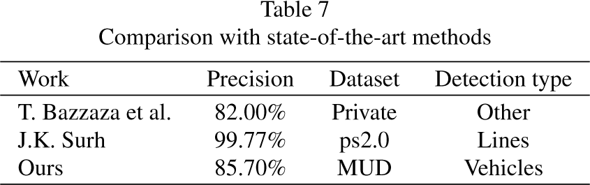
Comparison with state-of-the-art methods
As can be seen, the calibration step is the most time-consuming step, but as mentioned above, it is only performed during system initialisation. Regarding the time consumed by the vehicle detection phase, all systems are capable of being used in urban environments as the maximum allowed speed is 50 km/h (13.89 m/s). The slowest system is able to process images at 6.66 fps, which means that it can detect parking spaces every 2.3 metres, which is sufficient for our purpose.
Examples of the results obtained in the different variants of the proposed system. The first row refers to the complete model, the second to the no city modeling, the third to no filtering of moving vehicles and fourth to the no maximum depth constraint variant. Vehicle detections are marked with blue boxes. The ground truth labels for parking spaces are also marked with red dotted boxes. The parking spaces estimated by the system are marked with green dashed boxes.
The Málaga Urban Dataset (MUD) [41] provides data captured from a vehicle equipped with a stereo camera and five laser scanners pointing in different orientation, among other sensors. The information was obtained during a 36.8 km route with a frame rate of 20 fps at a resolution of 1024
In this work, we use 200 left frames of the stereo camera dataset for parameter setting (dataset A) and 17403 for testing (dataset B). These images are manually labeled with all possible parallel parking spaces. Signs prohibiting parking, crosswalks, and possible obstacles blocking parking have not been taken into account. As a result, 86 labels in 71 images in set A and 14687 in set B in 8307 images have been obtained. Figure 5 shows some examples of labeled parking gaps (red boxes).
As previously mentioned, detecting parking spaces in uncontrolled areas poses a challenge due to the diverse scenes that can arise. Various factors, such as curved streets, traffic violations, different types of parking spaces, crosswalks, prohibited parking zones, and obstacles in parking areas, must be considered. To focus on specific scenarios, we used scenes with mostly straight streets, and exclude crosswalks, obstacles, and no-parking zones. Only locations permitting parallel parking were labeled as parking zones. Despite these limitations, we aimed to simulate realistic environments, considering different lighting conditions and traffic situations.
Parameter setting
This preliminary experiment is designed to find the best parameter setting of the system. For this purpose, a search was carried out for the following two parameters:
Minimum parking space length. This parameter establishes the minimum distance between consecutive parked vehicles to consider that there is a parking space between them. A preliminary analysis revealed that this distance could not be less than three distance units, according to the depth estimation network used. As a consequence, and taking into account that a parking gap needs to be somewhat larger than a vehicle length, the system has been tested with values between four and seven units for this parameter. The larger this value is set, the smaller the number of false positives, but also the higher the number of false negatives. Table 3 (detection problem) and Table 4 (classification problem) show the evolution of false positives, true positives and false negatives as a function of the minimum parking space size, keeping all other variables fixed. Maximum distance for analysis. The accuracy of parking space detection decays as depth increases. This is due to the accuracy of the depth estimation network, that decays when the distance to the camera gets larger. For this reason, the system is configured to ignore information beyond a certain depth. We tried values of 20 and 30 units for this parameter.
We have conducted this experiment on data set A to test four different possible combinations of these two parameters. The results are shown in Table 5 for the detection problem and Table 6 for the classification problem. We observe that the optimum parameter values are 5 units for the minimum parking space length and 20 units for the maximum distance for analysis. These values are then used for the rest of experiments on the data set B.
This section aims to validate the results obtained on the dataset A using the same parameter setting on the dataset B. Figure 6 summarizes the obtained results. The system achieves an F1 score of 0.726 with 8993 TP, 3362 FP and 3422 FN in the detection problem. As expected, results are better for the classification problem, obtaining an F1 score of 0.847 and an accuracy of 0.857 percent points, with 6892 TP, 1322 FP, 1160 FN and 8029 TN. The proposed method is comparable with other state-of-the-art works as can be seen in Table 7.
Ablation study
We have performed an ablation study to test the influence of each component of the APSD system on the final results. These tests have been conducted on the dataset B. We have tested the following three system variations:
No city modeling. City modeling informs the areas where parking is allowed, so, without it, the detection of free parking spaces is carried out anywhere. No filtering of moving vehicles. In this variation, vehicles in circulation are not removed and, therefore, the system considers them as parked vehicles. No maximum depth constraint. This variation tries to detect free parking space vehicles at any depth.
We report F1-score and accuracy for detection and F1-score for classification as well as TP, FP, FN and TN. Figures 7.a and 7.b show the obtained results for the detection problem, while Figs 7.c and 7.d for the classification problem.
In absence of the city model, F1 Score decays 0.266 points for the detection problem. In regards to the classification problem, F1 score and accuracy are reduced by 0.228 points and 0.357 respectively. These results are due to the large increase in false positives.
Next, the Filtering Moving Vehicles phase is eliminated, decreasing F1 Score by 0.001 percent points. However, the results in the classification problem do not change. In both problems a reduction in true positives is observed.
Finally, the effect of maintaining the information at any depth is tested. We observe a reduction of 0.101 points of F1 Score in the detection problem and 0.031 in the classification problem. For the latter problem, accuracy decrease 0.028 points.
In this work we provide a computer vision-based Automatic Parking Space Detection (APSD) system. The system is made of specialized subsystems, some of them are machine learning-based methods (specifically, deep networks) and some are inspired by expert knowledge modelling (implemented as rule-based systems). We delegate some decisions to the system components, e.g. the detection network decides on the classes of vehicles detected, such as motorbikes, trucks, vans or cars. The task is far from trivial, mainly due to the fact that it is not possible to characterize parking gaps with only visual features and depth estimation using monocular cameras is not precise enough. We present an experimental analysis that includes a preliminary experiment to set the system parameter values and an ablation study. In this work we consider two related problems: detection (determine the position of the parking space) and classification (determine if there are parking spaces in an image). Our experimental findings reveal that our method effectively identifies parking spaces, even though it exhibits a high number of false positives. To address this issue, we propose an adaptive threshold for the minimum parking space size based on current traffic conditions. While an overly restrictive threshold may impact detections, our goal is to deploy the system across a fleet of vehicles. This allows us to validate parking information under diverse circumstances. Another challenge lies in camera calibration, which will be refined or potentially eliminated in future work through modifications on the expert systems. Additionally, we aim to enhance inference times by exploring alternative knowledge systems [42], neural networks [43, 44] or optimizing the existing ones. Although our system does not achieve accuracy levels comparable to the parking space detection state of the art methods for controlled scenarios, it excels in uncontrolled conditions and lays the foundation for solutions requiring minimal hardware infrastructure.