Sage Journals: Discover world-class research

Abstract

Left bundle branch block is a cardiac conduction disorder that occurs when the electrical impulses that control the heartbeat are blocked or delayed as they travel through the left bundle branch of the cardiac conduction system providing a characteristic electrocardiogram (ECG) pattern. A reduced set of biologically inspired features extracted from ECG data is proposed and used to train a variety of machine learning models for the LBBB classification task. Then, different methods are used to evaluate the importance of the features in the classification process of each model and to further reduce the feature set while maintaining the classification performance. The performances obtained by the models using different metrics improve those obtained by other authors in the literature on the same dataset. Finally, XAI techniques are used to verify that the predictions made by the models are consistent with the existing relationships between the data. This increases the reliability of the models and their usefulness in the diagnostic support process. These explanations can help clinicians to better understand the reasoning behind diagnostic decisions.

Keywords

LBBB diagnosis cardiac resynchronization therapy outcome spatial variance correlation analysis

1. Introduction

Automated ECG-based diagnosis is a classical field [1, 2, 3] with recent improved research due to the advances in Artificial Intelligence. Left bundle branch block is a cardiac conduction disorder that occurs when the electrical impulses that control the heartbeat are blocked or delayed as they travel through the left bundle branch of the cardiac conduction system. This results in a characteristic electrocardiogram (ECG) pattern, which progresses from incomplete LBBB (LBBB) to strict LBBB (sLBBB), defined by a prolonged QRS duration, a QS or rS pattern in the QRS complexes at leads V1 and V2 and the presence of mid-QRS notch/slurs in 2 leads within V1, V2, V5, V6, I and aVL [4]. sLBBB is associated with various underlying cardiac conditions, including hypertension, coronary artery disease, cardiomyopathy, and valvular heart disease. The clinical significance of sLBBB lies in its potential to cause cardiac dysfunction and the risk of developing heart failure, arrhythmias, and sudden cardiac death.

Recently, sLBBB has gained much attention since it was associated with clinical outcome of cardiac resynchronization therapy (CRT). CRT is a treatment for individuals with heart failure and conduction abnormalities. It is accomplished by a biventricular pacemaker that delivers electrical impulses to both the left and right ventricles, which helps synchronize their contractions and improve cardiac function. sLBBB was linked to improvements in CRT either in simulations [5] or patient studies [6, 7]. Accompanying this revision, an initiative in 2018 called for algorithms to detect strict LBBB in a full automatic way [8]. In general, automatic diagnosis of LBBB requires the correct detection of the morphological features that separate sLBBB from LBBB, grouping the latter with no LBBB at all. However, some individuals with LBBB may eventually develop sLBBB. This progression can occur due to the worsening of underlying cardiac disease, such as hypertension, coronary artery disease, or cardiomyopathy, or due to the development of scar tissue in the left ventricle. Therefore, it is important to identify and manage any underlying cardiac conditions that may be associated with the ECG changes. This can help prevent complications and improve patient outcomes.

The diagnosis of left bundle branch block can also be made using machine learning (ML) algorithms applied to ECG data. Studies have shown that machine learning algorithms can be highly accurate in diagnosing left bundle branch block from ECG data, with reported acuracies ranging from 70% to 82% [8]. Even though ML models can speed up the LBBB diagnosis, they generally act as black boxes, giving poor clues about the physiopathological processes underlying incomplete or strict LBBB. To overcome this flaw, techniques of Explainable machine learning (XAI) have arisen.

XAI [9, 10, 11, 12] refers to a set of techniques and methods used to make machine learning models and their predictions more transparent and interpretable to human users. The need for XAI arises from the increasing complexity of machine learning models, such as deep neural networks, which can have millions of parameters and layers that are difficult for humans to understand. XAI techniques [12] can be used to extract meaningful information from these models and provide explanations for their behavior. One of the most common XAI techniques is the use of feature importance methods, which identify the features in the input data that are most important for the model’s predictions. This can provide insights into the model’s decision-making process and help identify potential biases or errors in the model. Another widely used feature attribution method is Shapley values[13, 14], which, in addition to global explanations, allow for local explanations, i.e., determining the influence of each feature on a specific prediction. XAI can be useful in diagnosing Left Bundle Branch Block by providing insights into how machine learning algorithms make predictions and identifying the factors that contribute to the prediction.

Although there is a gap between making the correlations learned by a model transparent and establishing a causal relationship of why something happened [15], XAI techniques, used in conjunction with domain experts, can be useful to increase the trustworthiness in the models and identify the features in ECG data that are most important for the prediction of LBBB, providing valuable information to clinicians.

In this paper, a reduced set of biologically inspired features extracted from ECG data is proposed and used to train a variety of machine learning models for the LBBB classification task. Then, different methods are used to evaluate the importance of the features in the classification process of each model and to further reduce the feature set while maintaining the classification performance of the models. The performances obtained by the models using different metrics improve those obtained by other authors in the literature on the same dataset. Finally, XAI techniques are used to verify that the predictions made by the models are consistent with the existing relationships between the data. This increases the reliability of the models and their usefulness in the diagnostic support process.

The rest of this paper is organized as follows: Section 2 and subsections introduce the proposed methodology, the dataset structure, and the feature extraction and preprocessing algorithms. Section 3 contains the results obtained in the classification process by all the models and strategies, including a dedicated Section 3.4 for the explainability results. Section 4 contains a detailed discussion of the results in comparison with other approaches in the bibliography. Finally, Section 5 summarizes the conclusions, main contributions, and future work.

2. Materials and methods

2.1 Methodology

Figure 1.

Proposed methodology.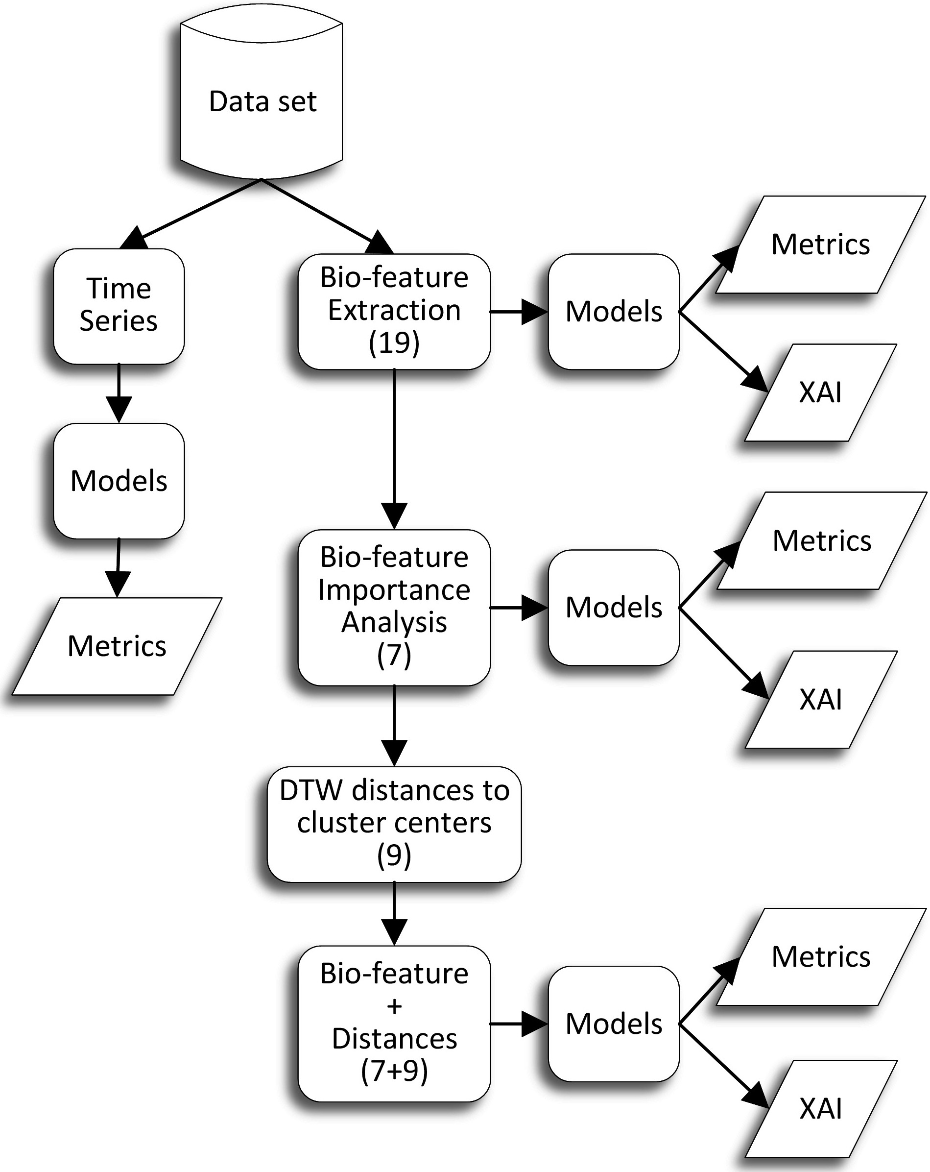

The proposed methodology is summarized in Fig. 1. The ECG dataset used in this work is publicly available at the Telemetric Holter Warehouse project (see Section 2.2 for details). In a first preprocessing step, the ECG data were transformed into vectorcardiographic space time series (Section 2.3). We then used some of the state-of-the-art algorithms specifically designed for time series classification to train machine learning models to detect three classes: NoLBBB, LBBB and sLBBB (Section 3.1). These models were supposed to be the best performing and achieve the highest classification accuracy, since they have all the available information of each data sample (800 timesteps $\times$ 3 timeseries). We used these metrics as a baseline to compare and benchmark the performance of the models developed in the further research.

The drawback of models that process time series directly, or that transform them into hundreds or thousands of statistical features automatically extracted from the time series [16], is that they are very complex, slow to train, and difficult to interpret. This is because the extracted features, if any, generally have no semantic value in the application domain, or even if they do, it is difficult for a human to analyze and understand the relationships between the (typically) hundreds of such variables that the algorithms extract and process.

Therefore, our research was aimed at extracting a reduced set of biologically meaningful features that could encode most of the information contained in the time series. In a first attempt, we computed a set of 19 bio-inspired features (defined in Sections 2.3 and 2.4). We then performed a correlation analysis to determine redundant features and a feature importance analysis using several algorithms to determine the most relevant variables for some classification models (Section 3.2). This resulted in a new reduced dataset of just 7 features for each sample.

Finally, we wanted to test whether the results on the features dataset could be improved using knowledge extracted from the time series. To this end, we used a clustering algorithm on the time series dataset to find the centroids (a kind of representative time series for each class) using the DTW [17] distance. Next, we used again the DTW to compute the distance of each time series to the centroids of each cluster. Finally we created a new dataset with 16 features, the 7-biologically relevant features, plus the 9 distances to the clusters.

We then trained machine learning models on the three bioinspired datasets and compared their performance metrics among themselves and with the time series models. In addition, we compare our results with those of other works in the literature (that deal only with the simpler case of binary classification). Finally, a post hoc explainability analysis was performed using SHAP values (Section 3.4) to determine whether the predictions made by the models were consistent with the existing relationships that could be observed in the data.

2.2 Database

Data were obtained from the E-OTH-12-0602-024 database, publicly available at the Telemetric Holter Warehouse project (THEW) [18], as part of the initiative of the International Society for Computerized Electrocardiology (ISCE), in 2018 [8]. Data comprise 602 10-second ECG recordings of heart failure patients included in the MADIT-CRT clinical trial. The 12-lead high-resolution ECGs were recorded before CRT implantation using 24-hours Holter recorders (H12 $+$ , Mortara Instruments, Milwaukee, WI, USA) with Mason-Likar lead configuration (the Mortara system provides 10 electrodes and records 8-lead signals [I, II, V1–V6] the other 4 leads are calculated). The sampling frequency was 1 kHz and amplitude resolution 3.75 microVolts. These data are from the MADIT-CRT trial conducted at the University of Rochester (Rochester, NY), and contained 302 strict LBBB, 184 incomplete LBBB and 74 no LBBB records. It is worth mentioning that we have ruled out 41 repeated records from the dataset, which were originally included for consistency purposes in the ISCE initiative.

2.3 ECG preprocessing

Table 1
Transformation matrix for Inverse Dower transformation (IDT).

Lead	V1	V2	V3	V4	V5	V6	I	II
$x$	$-$ 0.172	$-$ 0.074	0.122	0.231	0.239	0.194	0.156	$-$ 0.010
$y$	0.057	$-$ 0.019	$-$ 0.106	$-$ 0.022	0.041	0.048	$-$ 0.227	0.887
$z$	$-$ 0.229	$-$ 0.310	$-$ 0.246	$-$ 0.063	0.055	0.108	0.022	0.102

ECG data were transformed to the vectorcardiographic space (VCG) by means of the inverse Dower matrix as shown in Table 1. This transformation poses the orthogonal leads, $x$ , $y$ , $z$ , as linear combinations of the eight linearly independent ECG leads [19].

Signals were delineated by means of a wavelet-based algorithm using the WT-delineator library in Python [20]. The delineation algorithm detects the onset and offset of the QRS and T-wave, from which the QRS and T loops were constructed. In most of the cases, a manual correction was needed afterwards due to extremely aberrant ECG morphologies. From the latter ECG waves, a set of 19 features were obtained, as follows.

2.3.1 QRS-T angles

QRS-T angles were obtained for the planes $x y$ , $x z$ , $y z$ and for the volume $x y z$ . Following obtention of the QRS and T templates by ensemble averaging, the vectorcardiographic loops were constructed and aligned to the same origin, and dominant vectors defined as the maxima euclidean norm progressing between the onset and offset of the QRS and T loops in each of the following coordinate systems $x y$ , $x z$ , $y z$ and $x y z$ , as shown in Eq. (2) for the $x y$ plane:

$\displaystyle T_{\textit{opt}}=\arg\max_{n}\left\{d[n]\right\}$ (1)

with

$\displaystyle d[n]=\sqrt{(x[n]-x[0])^{2}+(y[n]-y[0])^{2}},$ (2) $\displaystyle\quad 0\leqslant n\leqslant t_{\textit{off}}$

where $x[0]$ and $y[0]$ are the QRS and T loop origins at leads $x$ and $y$ and $t_{\textit{off}}$ denotes the duration of the QRS or the T-wave templates, respectively. Dominant depolarization and repolarization vectors were then defined as $\textbf{QRS}_{\textit{opt}}/\textbf{T}_{\textit{opt}}=\{x[\textit{opt}],y[% \textit{opt}]\}$ . Once the QRS and T dominant vectors were determined, the angle between both was computed for every coordinate system as follows:

$\displaystyle\textit{Angle\_xy}=\left\{\!\frac{180}{\pi}\!\right\}\arccos\frac% {\langle\textbf{QRS}_{\textit{opt}},\textbf{T}_{\textit{opt}}\rangle}{\|% \textbf{QRS}_{\textit{opt}}\|\!*\!\|\textbf{T}_{\textit{opt}}\|}$ (3)

where $\langle\textbf{QRS}_{\textit{opt}},\textbf{T}_{\textit{opt}}\rangle$ denotes the inner product of the dominant vectors and $\|\textbf{QRS}_{\textit{opt}}\|$ , $\|\textbf{T}_{\textit{opt}}\|$ their $L_{2}$ norms in the $x y$ plane.

2.3.2 QRS-T areas

The QRS and T areas were calculated by summing up all the squared contributions from the intervening leads. Following, we provide the formula for the QRS area in the $x y$ plane:

$\displaystyle\textit{Area\_Rxy}[n]=\sum_{n=\textit{QRS}_{\textit{onset}}}^{% \textit{QRS}_{\textit{offset}}}(x^{2}[n]+y^{2}[n])$ (4)

2.3.3 Spatial variance

Spatial variance quantifies the maximal Euclidean distance of every lead within an ensemble from the lead ensemble average. In [21] there is a detailed description of the method for the ECG case. In this piece of work, all three VCG leads were utilized for spatial variance computing. Briefly, a 80-ms window centered around the QRS complex in lead $y$ segmented the QRS complexes for $x$ , $y$ , $z$ leads. Afterwards, spatial variance $\textit{SV}_{\textit{QRS}}$ was computed as

$\displaystyle\textit{SV}_{\textit{QRS}}=\arg\max_{n}\left\{\!\sqrt{x[n]^{2}+y[% n]^{2}+z[n]^{2}}\!\right\}\!,$

(5) $\displaystyle\qquad y_{\textit{peak}}^{\textit{QRS}}-40\ \text{ms}<n<y_{% \textit{peak}}^{\textit{QRS}}+40\ \text{ms}$
2.4 Correlation analysis

Table 2
Performance of the time series models

Model	Accuracy (%)	Precision (PPV) (%)	Sensitivity (%)	F1-score (%)
Rocket [23]	0.837500	0.860393	0.817677	0.832779
MRocket [24]	0.798214	0.836356	0.791376	0.807131
HIVECOTEV2 [25]	0.807143	0.841952	0.806571	0.819052
RRotForest [26]	0.826786	0.861584	0.807600	0.825459
DrCIF [27]	0.700000	0.696179	0.694063	0.689931
TDE [28]	0.812500	0.850251	0.794246	0.815504
CIF [27]	0.823214	0.858199	0.813357	0.827973
KNNTSC [29]	0.764286	0.790478	0.777579	0.780081

Table 3

List of 19 scalar features extracted for each record in the ECG dataset (upper), and the 7 most relevant features finally selected (lower)

Bio-inspired features
Angle_xy	Area_Rxy	Area_Txy	Argument_xy	Width_xy	Var_max
Angle_xz	Area_Rxz	Area_Txz	Argument_xz	Width_xz
Angle_yz	Area_Ryz	Area_Tyz	Argument_yz	Width_yz
Angle_xyz	Area_Rxyz	Area_Txyz
Most important features
	Area_Rxz	Area_Txz	Argument_xz	Width_xz
	Area_Ryz	Area_Tyz		Width_yz

Correlation analysis between leads also contributes to spatial heterogeneity, restricted to pairs of leads. In preserved conduction patients, the intrinsic deflections of both leads are conserved, then the correlation signal will be centered at zero ms. In the presence of conduction disorders, however, the maximum of the cross-correlation signal will present a latency. The original correlation marker was presented on ECG leads $I I$ and $V_{6}$ in [22] and herein adapted to the VCG case. The maximum argument of the cross-correlation signal (Argument_xy, in ms) between leads $x$ and $y$ was computed as follows:

$\displaystyle\textit{Argument\_xy}=\arg\max_{k}\left\{{\textit{Xcor}_{xy}[k]}\right\}$ (6)

with

$\displaystyle\textit{Xcor}_{xy}[k]=\sum_{n=-M+k}^{M-k}x^{\textit{QRS}}[n+k]y^{% \textit{QRS}}[n],$ (7) $\displaystyle\qquad\text{with}\ M=300\ \text{ms}$

The same computation was accomplished for the pair of leads ${xz}$ and ${yz}$ .

On the other hand, the width of the cross-correlation signal (Width_xy, in ms) was measured at 0.7*peak amplitude of the correlation between pair of leads ${xy}$ , ${xz}$ and ${yz}$ .

3. Results

3.1 Classification for time series dataset

In order to have some baseline models to compare, several time series classification models have been developed over leads $x$ , $y$ and $z$ . The dataset was therefore organized as an array of shape [560, 800, 3] ([samples, timesteps, features]). Classification was based on three classes: NoLBBB, LBBB and sLBBB.

For the development of the time series models, we used the sktime[16] framework that has more than two hundred dedicated time series algorithms for classification, regression, clustering and anomaly detection. We selected some of the most promising models to test our dataset such as KNNTSC, a KNN (K-Nearest Neighbors) Time Series Classifier using DTW (Dynamic Time Warping) as the distance metric; CIF and DrCIF, which are two variations of the Canonical Interval Forest classifier; TDE (Temporal Dictionary Ensemble) a model that uses a bag of words representation from the Fourier Transform of the time series; RRotForest (Random Rotation Forest), that builds a forest of trees on random portions of the data transformed in features using PCA (Principal Component Analysis); HIVECOTEV2, a meta ensemble of several classifiers (DrCIF and TDE between others) that work on different domains; and finally, ROCKET (RandOm Convolutional KErnel Transform) and MultiROCKET, that use random convolutional kernels to transform time series data and then trains a linear classifier on the transformed features, which represent nowadays the state of the art in common time series classification benchmarks.

3.2 Identification of relevant bio-inspired features

As mentioned before, our main objective was the extraction of relevant features from the ECG records that have a predictive power similar or better than the time-series models but are simultaneously smaller in number, easier to train, and more understandable for the physicians. To this purpose, from the ECG time-series, a total of 19 bio-inspired features were extracted for each record as explained in Section 2.3 and used for the bio-inspired features tabular dataset, thus having a size of [560, 19] ([samples, features]). The list of extracted features is shown in the upper part of Table 3.

Figure 2.

Boxplots for physiological features on classes NoLBBB, LBBB and sLBBB. 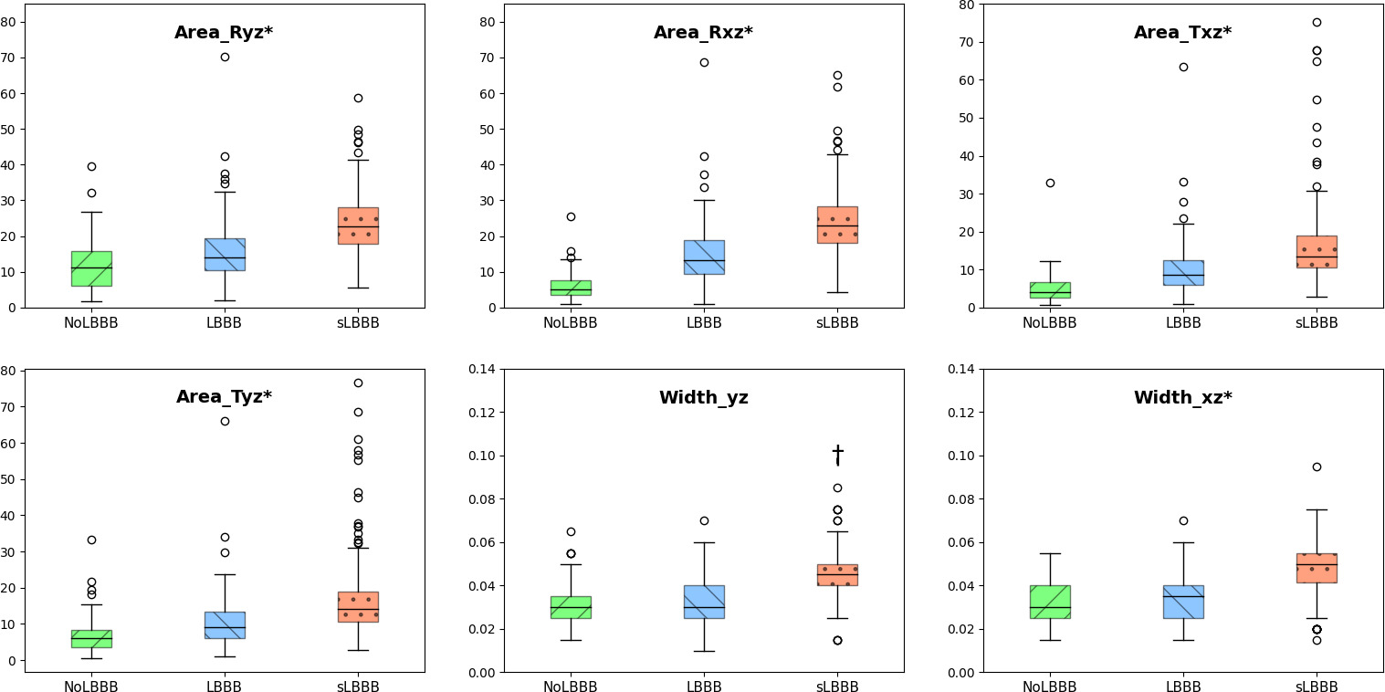${}^{*}$ Features resulted significantly different ( $p<$ 0.05) among all three classes, except for Width_yz, which resulted significantly different among NoLBBB and sLBBB. ANOVA with Bonferroni posthoc test for multiple comparisons of independent groups.

Figure 2 shows the boxplots of 6 representative physiological features used in the classification for NoLBBB, LBBB and sLBBB classes. Note that all of the features but Width_yz resulted in significantly different in pairwise comparisons among all three classes by the Bonferroni posthoc test following Analysis of Variance (ANOVA). In particular, areas either in the QRS or T loops significantly increased from NoLBBB to sLBBB in a progressive way ( $p<$ 0.001). Similarly, Width_xz did increase significantly among all classes ( $p<$ 0.05) although Width_yz provided statistical significance between NoLBBB and sLBBB only. In addition, Fig. 3 shows the cross-correlation between QRS complexes in leads $x$ and $y$ for a NoLBBB, a LBBB and a sLBBB patient. Note that all three classes presented clearly different VCG patterns (upper panel), which in turn, produced very different cross-correlation signals and QRS and T loops in the VCG (lower panel). It is worth mentioning that all patients in the dataset presented heart failure. Thus, even those belonging to the NoLBBB class can show a VCG record that differs from a healthy VCG record.

Figure 3.

Representative example of physiological features for NoLBBB, LBBB and sLBBB patients.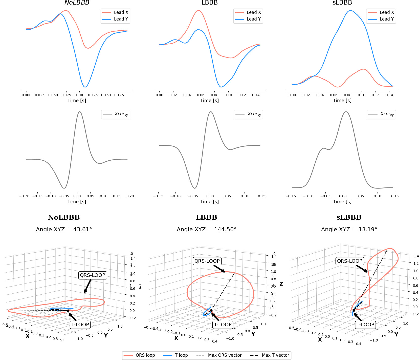

A direct exploration of the physiological features showed that some of these were highly correlated, therefore a multicollinearity analysis was performed. Multicollinearity can lead to unstable and unreliable estimates of regression coefficients [30] and makes it difficult to distinguish the effects of each independent variable in the target, that is, it can hinder the explainability of the model. We used Pearson’s correlation coefficient and VIF [31] (Variance Inflation Factor) to determine the strength of multicollinearity and performed an iterative feature selection process to select a subset of independent variables that were not highly correlated. This feature selection process was complemented with a feature importance analysis. Feature importance refers to techniques that assign a score to independent features based on how useful they are at predicting a target variable. Therefore, this is a way to understand which features have the most impact on a model’s prediction. There are several methods for calculating feature importance, among others, the following were used in our case. Tree-based algorithms automatically compute importance scores (TIS) during training based on the reduction of the split points, like Gini impurity or entropy, that could be used to determine feature importance [32]. Univariate Feature Selection [33] (UFS) uses statistical test to select the features that are more correlated with the output variable. Recursive feature elimination [34] (RFE) recursively removes input features and fits a model on the remaining ones, finally it uses the model’s accuracy or any provided metric to select the subset of features that better predict the target variable. Permutation Feature Importance (PFI) [35] works by calculating the increment in the model’s prediction error when a feature value is randomly permuted. Finally, SHAP (SHapley Additive exPlanations) [14] is a method that can be used to determine the importance of features in a machine learning algorithm. It is based on the computation of SHapley values, which measure the influence of each feature on the model’s prediction. Therefore, SHAP is also one of the most relevant ML explanation methods.

As those feature importance estimators depend on the model used to predict the target variable, we used 3 of the most widely used algorithms for tabular datasets: Xgboost, Random Forest and SVM, a classical method [36, 37] with recent applications in many different fields [38], to build 3 base-models and evaluated all the mentioned feature importance estimators on them.

Figure 4.

Recursive feature elimination with CV for automatic tuning of the number of features. Model’s accuracy greatly improves from using 1 up to 7 features, were it begins to saturate. Figure shows also the list of the the 7 selected features.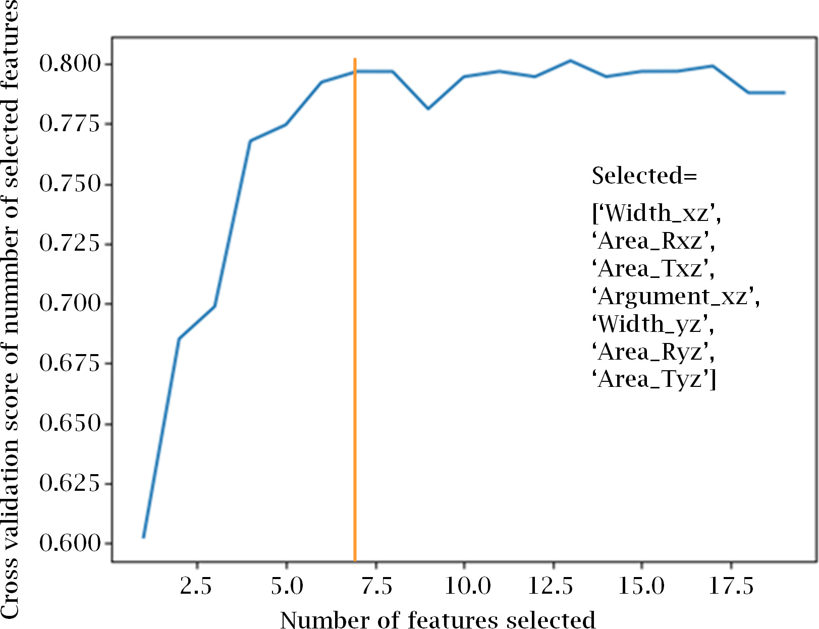

Figure 5.

Determining feature importance for the Random Forest model: (a) RF tree split-entropy. (b) Univariate selection using ANOVA F-value. (c) Permutation Feature Importance. (d) SHAP values average impact on model output by class.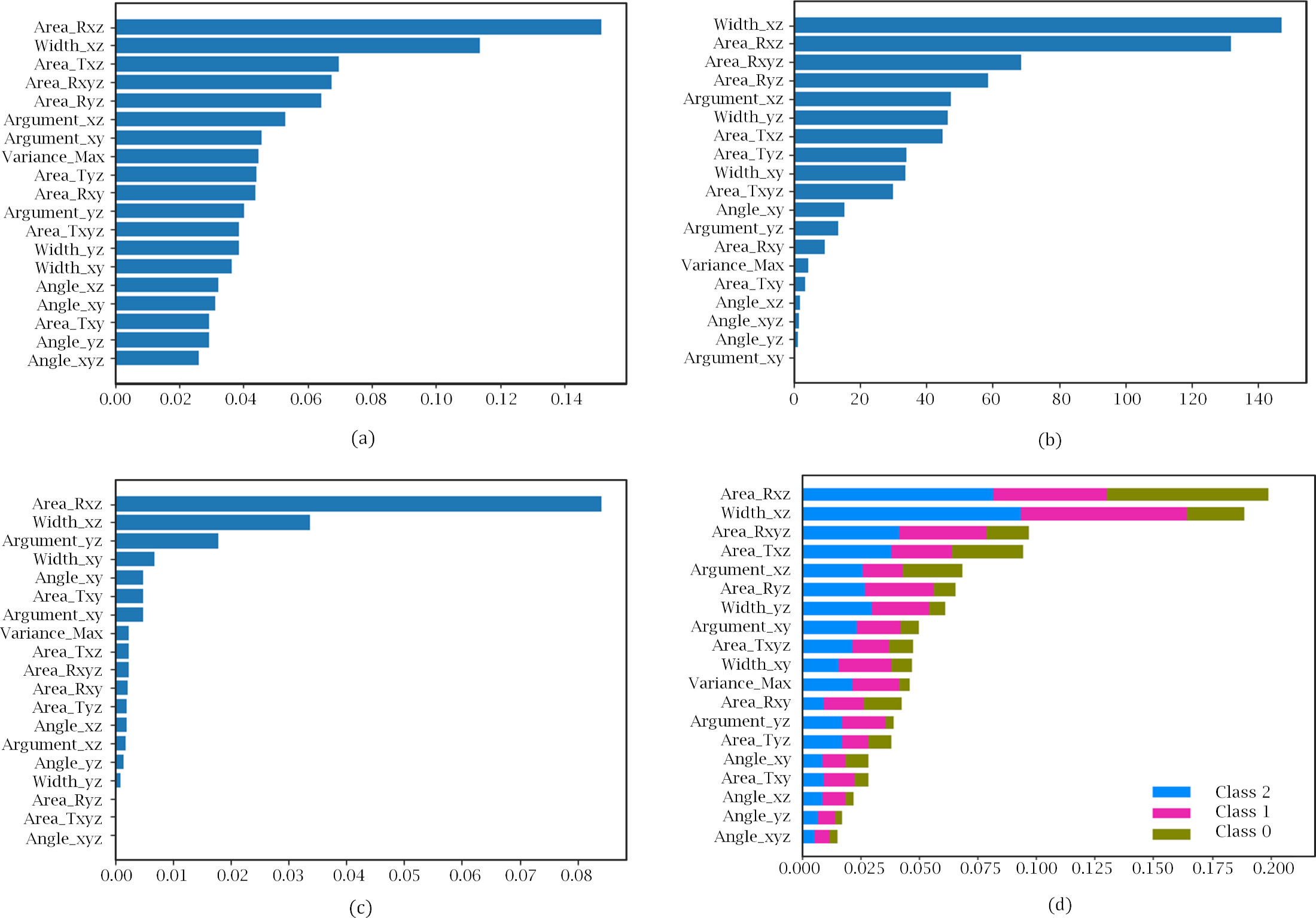

From the results of RFE with 5-fold cross-validation (CV) we estimated the optimum number of features as 7, as seen in Fig. 4. To select the most relevant and less correlated features, we took into consideration the 10 most important features provided by each method and model, and selected those that were common to a majority of them.

As an example, Fig. 5 shows the contribution for a Random Forest model. TIS, UFS and SHAP have 6 features in common between the first 10, while RFE has 5, and PFI, 4. The result of this analysis was a subset of relevant features, shown in the bottom part of Table 3, that we used to train our machine learning models on, as explained in the next section.

Finally, we wanted to test if results on the features dataset could be improved using knowledge extracted from the time series. To this point, we used a clustering algorithm on the timeseries dataset to automatically find the centroids of 3 clusters within the data. For time series, each centroid can be seen as representing the “mean observation” within a cluster across all the time steps, an is therefore another series. In multivariate timeseries dataset, the centroids could be used to understand the average behavior of each variable within each cluster.

We used the KNNTSC algorithm available in sktime, a version of the classical KNN for time series data, and fitted the model using both Euclidean an Dynamic Time Warping (DTW) distances. DTW [17, 39] is reportedly a better metric for time series clustering because it gives more robustness to the similarity computation. It replaces the one-to-one point comparison used in Euclidean distance with a many-to-one (and vice versa) comparison. This allows DTW to compare time series of different lengths and be invariant to time shifts, which is important when comparing time series data.

Next, we used again the DTW to compute the distance for each time series to the centroids of every cluster. Therefore, for each record in the dataset consisting in 3 timeseries (X, Y and Z components), we obtained 9 scalars: the DTW distance or each component to each centroid. Finally we created a new dataset with 16 features for each sample, consisting of the 7-biological relevant features, plus the 9 distances to the clusters.

3.3 Classification using relevant bio-inspired features

Table 4
Metrics of the base-models for the 19-features dataset

Model	Abrev.	Accuracy	Precision	Sensitivity	F1-score
Linear discriminant analysis	lda	0.8162	0.8293	0.8162	0.8105
Extra trees classifier	et	0.8085	0.8191	0.8085	0.8045
Random forest classifier	rf	0.7933	0.8043	0.7933	0.7877
Extreme gradient boosting	xgboost	0.7908	0.8000	0.7908	0.7831
CatBoost classifier	catboost	0.7881	0.7974	0.7881	0.7835
Light gradient boosting machine	lightgbm	0.7807	0.7826	0.7807	0.7727
Ridge classifier	ridge	0.7576	0.7610	0.7576	0.7437
Gradient boosting classifier	gbc	0.7575	0.7626	0.7575	0.7534
Logistic regression	lr	0.7550	0.7556	0.7550	0.7516
Quadratic discriminant analysis	qda	0.7474	0.7690	0.7474	0.7449
Decision tree classifier	dt	0.6862	0.6975	0.6862	0.6862
Ada boost classifier	ada	0.6787	0.6971	0.6787	0.6764
K neighbors classifier	knn	0.6758	0.6744	0.6758	0.6641
Naive Bayes	nb	0.6506	0.6926	0.6506	0.6533
SVM – linear kernel	svm	0.5715	0.5279	0.5715	0.4969

Development of models for the 3 bio-features datasets was accomplished in a two stage process. In the first stage, a set of 15 well-known Machine Learning algorithms were trained on the features dataset, using a simple train-test split approach (80%–20% respectively), and mostly default or common-use set of hyperparameters. From the results obtained, shown in Table 4, we selected the 4 better performing algorithms, LDA, ET, RF and Xgboost, for further fine tuning.

Fine tuning was carried out in the second stage by using the following procedure. For each of the 4 algorithms, we defined 500 unique models using different combinations of hyperparameters based on a standard grid search. Each model was in turn trained using a 10-fold cross-validation schema, to ensure the consistence of the performance metrics.

For comparison purposes, we repeated this process for the original 19-features dataset, the 7-most-relevant features dataset and the 7-relevant features plus 9-distances-to-centroids dataset. In the end, 2000 different models were trained for each of the 3 feature-based datasets.

The 500 models of each machine learning algorithm were fitted and ordered by their mean accuracy over the 10 trained folds. We use accuracy in this case to select the best models, as it was the most relevant metric for our classification purposes and classes are not highly unbalanced, but F1-score would also had been a good choice. The scores of the best model for each algorithm on each of the 3 feature-based datasets are shown in Table 5. Precision, Sensitivity and F1-score have been averaged over the 3 classes.

Table 5

Metrics for the best performing models on the 3 bio-inspired features datasets, for the 3-classes classification task

Dataset	Model	Accuracy	Sensitivity	Precision	F1-score
19 features	lda	0.8162	0.8035	0.8249	0.7970
	et	0.8162	0.8162	0.8245	0.8152
	rf	0.8087	0.8087	0.8199	0.8047
	xgboost	0.8162	0.8162	0.8257	0.8097
7 features	lda	0.7602	0.7602	0.7718	0.7454
	et	0.7985	0.7985	0.8061	0.7936
	rf	0.8011	0.8011	0.8134	0.7979
	xgboost	0.8036	0.8036	0.8095	0.7996
7feat $+$ 9dist	lda	0.8110	0.8110	0.8220	0.8086
	et	0.8263	0.8263	0.8381	0.8232
	rf	0.8213	0.8213	0.8353	0.8197
	xgboost	0.8160	0.8160	0.8275	0.8129

Figure 6.

Feature dependence plots for the ET model on the 7feat+9dist dataset. Each row shows shap values for a given feature (Width_xz, area_Rxz, Area_Txz, Argument_xz), related to each class (left: NoLBBB, center: LBBB, right: sLBBB). Color corresponds to a second feature that has strongest interaction with the feature on the x-axis.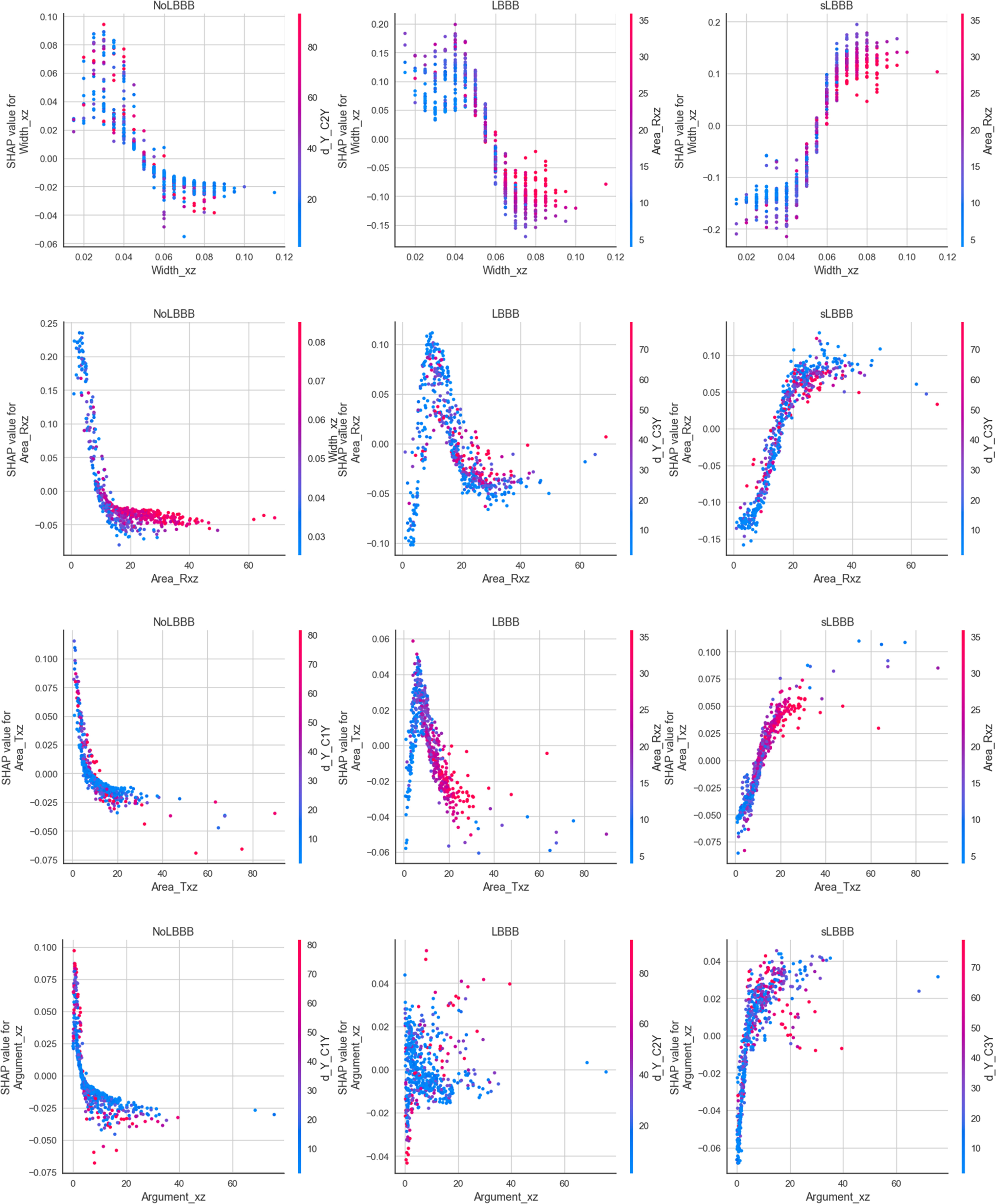

Figure 7.

Local explanation for sample 347. Top: 3 force plots (one for each class: 0 for NoLBBB, 1 for LBBB, 2 for sLBBB) of the Shap values for this sample visualize how the 7 bioinspired features contribute to a specific prediction. Each force plot shows the base value for the class and the contributions from each feature to the final prediction. Red arrows indicate positive contributions, while blue ones indicate negative contributions. The length of the arrow indicates the magnitude of the contribution. Bottom: 7 Kernel Density Estimate (KDE) plots visualize the distribution of the 7 bioinspired features, by class. Superimposed, a dotted-red vertical line marks the value of that feature for this sample. The 8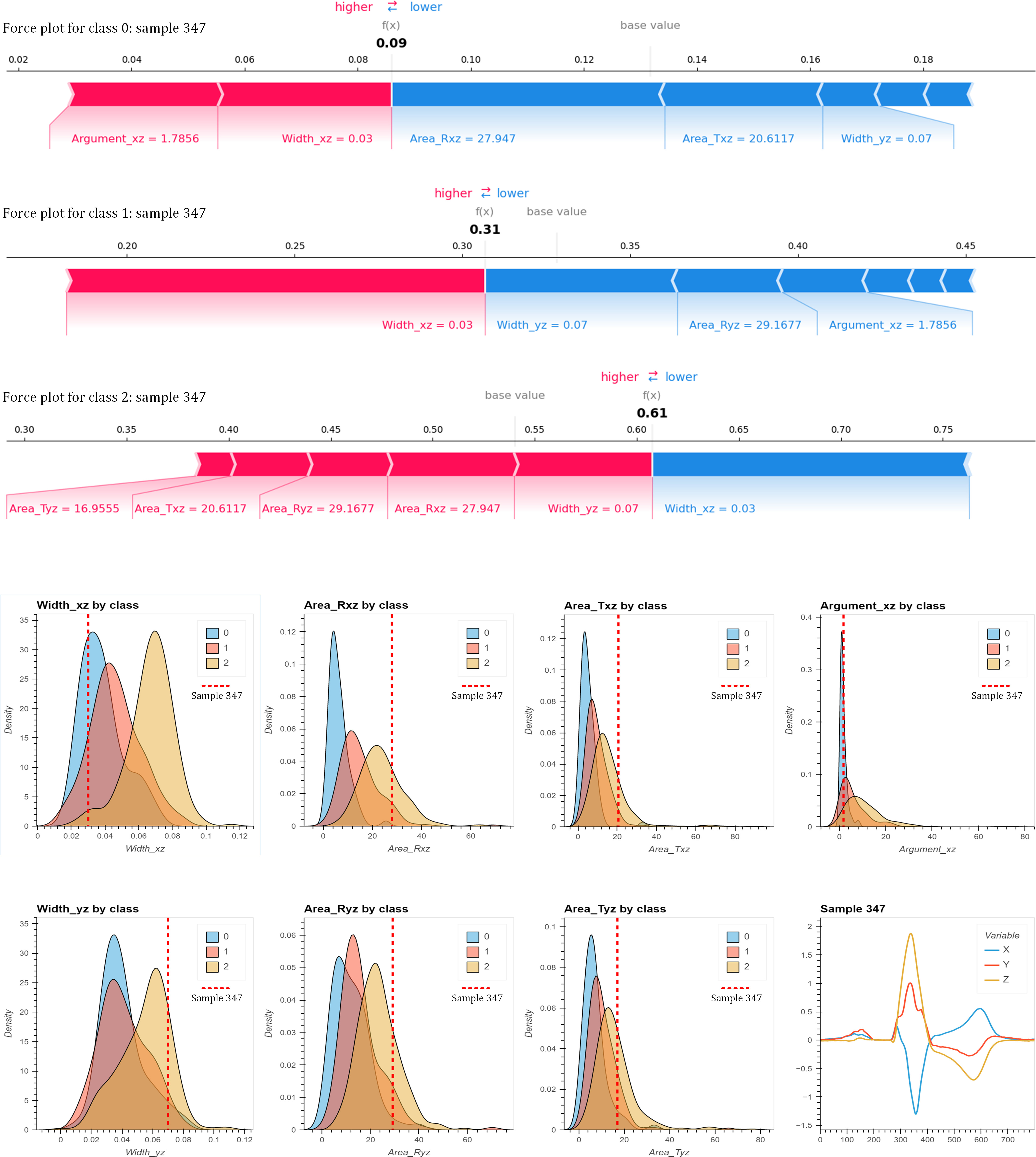 ${}^{\text{th}}$ plot shows the VCG representation of the ECG (in x, y and z axes) for this sample.

It can be observed that the performance for the 7-feature dataset is only slightly lower than for the 19-feature dataset. This suggests that the previous feature importance analysis was correct and that most of the variance in the dataset can be explained by just the 7 most relevant features. Moreover, the best performance is consistently obtained for the 4 metrics for the 7feat+9dist dataset, with the Extremely Randomized Trees (ET) algorithm getting the highest absolute scores for each metric. This seems to support the idea that the 9 distances help the algorithm to slightly improve its predictive power.

Compared with the time series models, it should be noted that the bio-inspired features dataset achieves a slightly lower accuracy (82.64% vs. 83.75% for the best performing models), albeit still comparable, with the advantages of lower complexity and better explainability. To determine whether this difference is significant, a Kruskal-Wallis [40] hypothesis test was performed on the validation k-folds between the best models (accuracy over 80%) of both types, which resulted in p-values of 0.787, 0.974, 0.377 and 0.985 for the 4 metrics (accuracy, sensitivity, precision and F1-score respectively), all of them above 0.05. Thus, it can be affirmed that there is no significant statistical difference between the two cases, and our biological features are able to condense in a few values most of the information contained in the time series.

3.4 Explainability

One commonly used method to determine feature attribution is Shapley values. Shapley Values rely on examining how each feature influences the predicted value of a model by generating many predictions based on a partial set of the features used by the model and comparing the results of the predicted values. In our case, the Python library SHAP [14, 41, 42] was used for the computation of the Shapley values. As an example, the SHAP values for 4 of the 7 relevant features are shown in rows in Fig. 6. Each column corresponds to the shap values for each of the classes. Within each plot, each point is the shap value corresponding to one of the samples for that feature and class. Positive shap values indicate that the corresponding values of the feature would contribute positively to the classification of the sample as belonging to that class. Negative shap values would indicate that the values of that feature are decreasing the probability of belonging to that class.

Note that there are biological parameters that serve to discriminate one class from the other two, but not between those two (e.g. Width_xz would separate only sLBBB from the other two classes, and Argument_xz, would separate only the NoLBBB from the rest), while other parameters serve to discriminate between the 3 classes, such as Area_Rxz and Area_Txz.

For instance, for Width_xz lower than 0.06 seconds, there are positive SHAP values for NoLBBB and LBBB, while for values greater than 0.06 seconds, positive SHAP values appear for sLBBB, indicating sLBBB. Area_Rxz and Area_Txz are different. If values are lower than 16, points to NoLBBB, between 16 and 20 to LBBB, and greater than 20 to sLBBB. The values for Area_Txz ranging from 0 to 5 account for NoLBBB, from those 5 to 15 indicate LBBB, and those greater than 15 sLBBB. Finally, if Argument_xz is lower than 5 points to NoLBBB, while if greater than 5 LBBB or sLBBB. It is worth mentioning that the yz plane with its features Area_Rxz, Area_Txz and Width_yz have followed a similar but slightly weaker pattern than their counterparts in the $x z$ plane. Thus, the $x z$ plane has come out as the more significative plane and the set of all features was the combination that gave the best accuracy, up to 82.63% as previously described. These SHAP values can help clinicians to interpret the importance of each parameter for each patient based on their condition, etc.

In addition to global explanations, SHAP values can also provide local explanations, i.e., explanations of the model outcome (classification) for a single data sample. An example of this is shown in Fig. 7. The upper part of the figure shows 3 force plots corresponding to the 3 classes presenting the SHAP values for each of the 7 bioinspired features that explain the classification made by the model. This case corresponds to sample 347, labeled as class1 (LBBB), which the model has erroneously classified as class2 (sLBBB).

The force plots show that this sample was classified as class2 because SHAP values (Width_yz $=$ 0.07, Area_Rxz $=$ 27.94, Area_Ryz $=$ 29.16, Area_Txz $=$ 20.61 and Area_Tyz $=$ 16.95) contributed strongly (very positive values) towards that class, as can be seen in the force diagram for class 2. These same features logically contributed negatively to class0 and class1, as can be seen in the corresponding force diagrams. However, the value of Width_xz $=$ 0.02, together with the values of Argument_xz, contributed positively to classification as class1 (and even as class0, although to a much lesser extent), so the model finally classified it as class2.

We can try to compare the explanation that SHAP provides about the associations learned by the model with a basic statistical analysis of the data to see if the model is wrong or if the classification is consistent with the relationships that we can see in the data itself. This analysis has been performed in the lower part of Fig. 7, where the probability density functions (KDE) of each of the 7 bioinspired features are plotted for each of the classes.

In the KDE graphs, it can be seen how the values of the same features that contributed positively to belonging to class2 in the force graphs (Width_yz, Area_Rxz, Area_Ryz, Area_Txz and Area_Tyz) for this sample are indeed very typical of class2 , to a much greater extent than for classes 1 and 0. Therefore, these relationships have been correctly learned by the model.

KDE analysis also showed that Width_xz contributes positively to classes 0 and 1, which is also consistent with the model as can be seen from the corresponding force plots. However, the model considered that Argument_xz contributed positively to class0, but negatively, albeit very slightly, to class1, which in this case would be in disagreement with the observed distributions for this parameter.

4. Discussion

Table 6
Metrics for the best performing models on the 3 bio-inspired features datasets, for the binary classification task

Dataset	Model	Accuracy	Sensitivity	Precision	F1-score
19 features	lda	0.8622	0.8814	0.8728	0.8735
	et	0.8647	0.8959	0.8622	0.8776
	rf	0.8596	0.8959	0.8560	0.8738
	xgboost	0.8469	0.9335	0.8124	0.8676
7 features	lda	0.8544	0.8766	0.8598	0.8660
	et	0.8546	0.8532	0.8773	0.8634
	rf	0.8391	0.8528	0.8497	0.8505
	xgboost	0.8237	0.9100	0.7967	0.8477
7feat $+$ 6dist	lda	0.8521	0.8580	0.8726	0.8622
	et	0.8597	0.8816	0.8641	0.8712
	rf	0.8469	0.8673	0.8545	0.8595
	xgboost	0.8366	0.9054	0.8162	0.8569

To the best of our knowledge, there are no other works in the literature that use this dataset to classify LBBB into 3 classes. Therefore, to evaluate our strategy, we decided to apply the same procedures that produced Table 5 to the simpler case of binary classification, to allow a fair comparison with the literature (results shown in Table 6).

The results show an increase in the performance of all models with respect to the 3-class problem. The majority of them achieving an accuracy above the 85%. The Extremely Randomized Trees (ET) for the 19-feature dataset is the best model, in terms of accuracy (86.47%) and F1-score (87.76%). In this case, however, adding the 6 distances to the clusters provides a negligible improvement over the dataset with only the 7 most relevant features. In any case, its metrics fall below those of the original 19-feature dataset.

With respect to the results of other groups, although it is not possible to establish a direct correspondence since the experiments were performed under different conditions, our models for binary classification improve the results obtained by all participants in the International Society for Computerized Electrocardiology’s initiative for automated LBBB detection in terms of accuracy, sensitivity and precision. According to [8], the best accuracy reported by the 7 participants in the initiative was of 82% (with 69% sensitivity and 87% precision) [43]. In 2020, however, Yang et al. achieved a 88.7% accuracy, with a sensitivity $=$ 91.7%, and specificity $=$ 85.6% (PPV $=$ 87.2%, NPV $=$ 90.6%) by means of a 5-layer neural network fed by features selected from a random forest algorithm [44]. However, it is important to point the validation scheme used for getting the results. It is worth noting that we achieved a comparable performance by utilizing features that do not account for the morphological conditions that meet the sLBBB criteria, but others that reveal underlying processes secondary to LBBB or sLBBB, such as the shift in the intrinsic deflections [45] or the spatial dispersion originated in left conduction abnormalities [46].

The good results obtained for the binary classification problem validated the relevance of the extracted bioinspired features for the determination of the sLBBB presented in Section 2.3, which led us to apply the same strategy in the case of 3 classes. As explained in Section 3.3 and resumed in Table 5, for the 3-classes dataset we obtained a 82.63% accuracy and 82.32% F1-score, results similar to what other groups claim for the binary problem. At this point it is also worth mentioning that the ternary classification (NoLBBB, LBBB and sLBBB) presents quite a challenging problem, since differences among groups, in particular between LBBB and sLBBB can be very small. Despite these issues, we insist in a ternary classification, since we believe that early diagnose of mild LBBB may improve the natural evolution to sLBBB. Therefore, we give value to either sLBBB or LBBB diagnosis equally.

Regarding physiological features, we have separated those which contribute to differentiate three classes from those that discern only two. To begin with, notice that the lead $z$ turned out as the most promising lead to classify among all three classes, since it is involved in all the planes involved in the relevant physiological features. This is consistent with general vectorcardiographic criteria for LBBB patterns [47].

Analyzing the features by means of the feature importance obtained in Figs 5, 3 and dependence plots, as shown in Fig. 6, QRS area in the $x z$ plane appeared as one of the most valuable features. This is consistent with [48], who found a good correlation between sLBBB and QRS area. Indeed, they claim QRS area as a clearly defined parameter that should be used to optimize biventricular stimulation. More importantly, QRS area was reported to be associated with long-term outcome in CRT [49]. Following this reasoning, the T area (either in the $x z$ or $y z$ plane) outstood as a valuable feature. This fact was surprising, since repolarization parameters were rarely included in the literature to describe a conduction disturbance. The latter observation, however, makes sense, since it is sensitive to expect repolarization abnormalities secondary to a depolarization disturbance.

The contribution of parameters based on correlation analysis (Width_xz and Argument_xz), however, was useful just for binary classification, with a lower performance at the ternary problem. According to Fig. 6, Argument_xz was able to distinguish between NoLBBB versus both LBBB and sLBBB, but failed in the separation of the latter groups. The oppositte occured with Width_xz, which managed to differentiate sLBBB from the remaining classes, but presented similar SHAP values for NoLBBB and LBBB. This fact is not consistent with [50], where both parameters explained the electrical activation of the free wall of the left ventricle with an Adjusted $-R^{2}$ $=$ 0.78 in a mixed-effects model. This might be explained by the conjunction of both parameters, acting synergically in the model.

5. Conclusion

In this study, we have explored the potential of explainable artificial intelligence (XAI) in the detection of the three levels of left bundle branch block (LBBB) using physiological parameters. The results show that XAI can increase the performance of LBBB detection, and they can be used to provide also explainable and interpretable insights into the underlying physiological mechanisms.

We have shown that a reduced set of biologically inspired features extracted from ECG data can be used to evaluate the importance of the features in the classification process of each model and to further reduce the feature sets while maintaining the classification performance of the models. The performances obtained by the models using different metrics improve those obtained by other authors in the literature on the same dataset. Finally, XAI techniques have been used to verify that the predictions made by the models are consistent with the existing relationships between the data. This increases the reliability of the models and their usefulness in the diagnostic support process. Our results also highlight the importance of transparency and interpretability in AI-based medical applications, as they can help clinicians better understand the reasoning behind diagnostic decisions and facilitate trust and adoption of AI tools in clinical practice.

In future works we well refine our research with new methods as Neural Dynamic Classification algorithm, Dynamic Ensemble Learning Algorithm, Finite Element Machine for fast learning, and self-supervised learning [51, 52, 53, 54] for improving the results and explanations.Overall, our study shows that XAI has potential to revolutionize the way we diagnose and treat cardiovascular diseases, by providing accurate and interpretable insights into complex physiological mechanisms. Further research is needed to validate our findings in larger and more diverse patient populations, and to explore the potential of XAI in other medical domains.

Footnotes

Acknowledgments

The work reported here has been partially funded by Grant PID2020-115220RB-C22 funded by MCIN/AEI/ 10. 13039/501100011033 and, as appropriate, by “ERDF A way of making Europe”, by the “European Union” or by the “European Union NextGenerationEU/PRTR”. This research has been also funded by a PhD scholarship from the National Council of Science and Technology (CONICET) and by Grant 26-DI-FEIRNNR-2023 from Universidad Nacional de Loja (Ecuador).

References

Sankari

Adeli

. HeartSaver: A Mobile Cardiac Monitoring System for Auto-detection of Atrial Fibrillation, Myocardial Infarction and Atrio-Ventricular Block. Computers in Biology and Medicine. 2011; 41(4): 211-220.

Martis

Acharya

Adeli

. Current Methods in Electrocardiogram Characterization. Computers in Biology and Medicine. 2014; 48: 133-149.

Martis

Rajendra Acharya

Adeli

Tan

Tong

Chua

, et al. Computer Aided Diagnosis of Atrial Arrhythmia Using Dimensionality Reduction Methods on Transform Domain Representation. Biomedical Signal Processing and Control. 2014; 13: 295-305.

Strauss

Selvester

Wagner

. Defining Left Bundle Branch Block in the Era of Cardiac Resynchronization Therapy. American Journal of Cardiology. 2011; 107: 927-934.

Galeotti

van Dam

Loring

Chan

Strauss

. Evaluating strict and conventional left bundle branch block criteria using electrocardiographic simulations. EP Europace. 2014; 15: 1816-1821.

Emerek

Risum

Hjortshøj

Riahi

Rasmussen

Thomsen

, et al. New strict left bundle branch block criteria reflect left ventricular activation differences. Journal of Electrocardiology. 2015; 48: 758-762.

Hadjis

AlTurki

Proietti

Montemezzo

Bernier

Joza

, et al. Predicting response to cardiac resynchronization therapy: Use of strict left bundle branch block criteria. Pacing Clin Electrophysiol. 2019; 42: 431-438.

Zusterzeel

Vicente

Ochoa-Jimenez

Zhu

Couderc

Akinnagbe-Zusterzeel

Strauss

. The 43rd International Society for Computerized Electrocardiology ECG initiative for the automated detection of strict left bundle branch block. J Electrocardiol. 2018; 51: 25-30.

Gunning

. Explainable artificial intelligence (xai). Defense advanced research projects agency (DARPA), nd Web. 2017; 2(2): 1.

10.

Adadi

Berrada

. Peeking inside the black-box: a survey on explainable artificial intelligence (XAI). IEEE Access. 2018; 6: 52138-52160.

11.

Došilović

Brčić

Hlupić

. Explainable artificial intelligence: A survey. In: 2018 41st International convention on information and communication technology, electronics and microelectronics (MIPRO). IEEE; 2018. pp. 210-215.

12.

Arrieta

Díaz-Rodríguez

Del Ser

Bennetot

Tabik

Barbado

, et al. Explainable Artificial Intelligence (XAI): Concepts, taxonomies, opportunities and challenges toward responsible AI. Information fusion. 2020; 58: 82-115.

13.

Shapley

. A Value for n-Person Games. In: Kuhn

Tucker

, editors. Contributions to the Theory of Games II. Princeton: Princeton University Press; 1953. pp. 307-317.

14.

Lundberg

Lee

. A Unified Approach to Interpreting Model Predictions. In: Guyon

Luxburg

Bengio

Wallach

Fergus

Vishwanathan

, et al., editors. Advances in Neural Information Processing Systems 30. Curran Associates, Inc.; 2017. pp. 4765-4774. Available from: http://papers.nips.cc/paper/7062-a-unified-approach-to-interpreting-model-predictions.pdf.

15.

Lundberg

. Be Careful When Interpreting Predictive Models in Search of Causal Insights. Available from: https://towardsdatascience.com/be-careful-when-interpreting-predictive-models-in-search-of-causal-insights-e68626e664b6.

16.

sktime: a unified framework for machine learning with time series. Available from: https://github.com/sktime/sktime.

17.

Ding

Trajcevski

Scheuermann

Wang

Keogh

. Querying and mining of time series data: experimental comparison of representations and distance measures. Proceedings of the VLDB Endowment. 2008; 1(2): 1542-1552.

18.

Moss

Hall

Cannom

Klein

Brown

Daubert

, et al. Cardiac-Resynchronization Therapy for the Prevention of Heart-Failure Events. New England Journal of Medicine. 2009; 361(14): 1329-1338.

19.

Edenbrandt

Pahlm

. Vectorcardiogram synthesized from a 12-lead ECG: Superiority of the inverse Dower matrix. Journal of Electrocardiology. 1988; 21: 361-367.

20.

Ledezma

. WTdelineator. 2021. Available from: https://github.com/caledezma/WTdelineator.

21.

Bonomini

Ortega

Barja

Mangani

, et al. Electrical approach to improve left ventricular activation during right ventricle stimulation. Medicina (B Aires). 2017; 77: 7-12.

22.

Daniel

Emilio

Luis

Analía

Nicolás

Mazzetti

, et al. Novel implant technique for septal pacing. A noninvasive approach to nonselective his bundle pacing. Journal of Electrocardiology. 2020; 63: 35-40. Available from: https://www.sciencedirect.com/science/article/pii/S0022073620305525.

23.

Dempster

Petitjean

Webb

. Rocket: exceptionally fast and accurate time series classification using random convolutional kernels. Data Mining and Knowledge Discovery. 2020; 34(5): 1454-1495.

24.

Tan

Dempster

Bergmeir

Webb

. MultiRocket: Multiple pooling operators and transformations for fast and effective time series classification. arXiv preprint arXiv: 210200457. 2022.

25.

Middlehurst

Large

Flynn

Lines

Bostrom

Bagnall

. HIVE-COTE 2.0: A New Meta Ensemble for Time Series Classification. Machine Learning. 2021.

26.

Rodriguez

Kuncheva

Alonso

. Rotation forest: A new classifier ensemble method. IEEE transactions on pattern analysis and machine intelligence. 2006; 28(10): 1619-1630.

27.

Middlehurst

Large

Bagnall

. The Canonical Interval Forest (CIF) Classifier for Time Series Classification. In: 2020 IEEE International Conference on Big Data (Big Data). IEEE; 2020. pp. 1774-1783.

28.

Middlehurst

Large

Cawley

Bagnall

. The Temporal Dictionary Ensemble (TDE) Classifier for Time Series Classification. In: European Conference on Machine Learning and Principles and Practice of Knowledge Discovery in Databases. Springer; 2020. pp. 345-361.

29.

Geler

Kurbalija

Ivanović

Radovanović

. Time-Series Classification with Constrained DTW Distance and Inverse-Square Weighted k-NN. In: 2020 International Conference on INnovations in Intelligent SysTems and Applications (INISTA). 2020. pp. 1-7.

30.

Chan

JYL

Leow

SMH

Bea

Cheng

Phoong

Hong

, et al. Mitigating the Multicollinearity Problem and Its Machine Learning Approach: A Review. Mathematics. 2022; 10(8). Available from: https://www.mdpi.com/2227-7390/10/8/1283.

31.

Zuur

Ieno

Elphick

. A protocol for data exploration to avoid common statistical problems. Methods in Ecology and Evolution. 2010; 1(1): 3-14. doi: 10.1111/j.2041-210X.2009.00001.x.

32.

Menze

Kelm

Masuch

Himmelreich

Bachert

Petrich

, et al. A comparison of random forest and its Gini importance with standard chemometric methods for the feature selection and classification of spectral data. BMC Bioinformatics. 2009; 10(1): 213.

33.

Jović

Brkić

Bogunović

. A review of feature selection methods with applications. In: 2015 38th International Convention on Information and Communication Technology, Electronics and Microelectronics (MIPRO). 2015. pp. 1200-1205.

34.

Guyon

Weston

Barnhill

Vapnik

. Gene Selection for Cancer Classification using Support Vector Machines. Machine Learning. 2002; 46(1-3): 389-422.

35.

Breiman

. Random Forests. Machine Learning. 2001; 45(1): 5-32.

36.

Adeli

Yeh

. Explanation-Based Machine Learning in Engineering Design. Engineering Applications of Artificial Intelligence. 1990; 3(2): 127-137.

37.

Adeli

Balasubramanyam

. Expert Systems for Structural Design – A New Generation. Englewood Cliffs, New Jersey: Prentice-Hall; 1988.

38.

Luo

Paal

. A Data-Free, Support Vector Machine-Based Physics-Driven Estimator for Dynamic Response Computation. Computer-Aided Civil and Infrastructure Engineering. 2023; 38(1): 26-48.

39.

Dau

Silva

Petitjean

Forestier

Bagnall

Mueen

, et al. Optimizing dynamic time warping’s window width for time series data mining applications. Data mining and knowledge discovery. 2018; 32: 1074-1120.

40.

Kruskal

Wallis

. Use of ranks in one-criterion variance analysis. Journal of the American Statistical Association. 1952; 47(260): 583-621.

41.

Lundberg

Erion

Chen

DeGrave

Prutkin

Nair

, et al. From local explanations to global understanding with explainable AI for trees. Nature Machine Intelligence. 2020; 2(1): 2522-5839.

42.

Lundberg

Nair

Vavilala

Horibe

Eisses

Adams

, et al. Explainable machine-learning predictions for the prevention of hypoxaemia during surgery. Nature Biomedical Engineering. 2018; 2(10): 749.

43.

Smisek

Viscor

Jurak

Halamek

Plesinger

. Fully automatic detection of strict left bundle branch block. J Electrocardiol. 2018; 51: S31-S34.

44.

Yang

Gregg

Babaeizadeh

. Detection of strict left bundle branch block by neural network and a method to test detection consistency. Physiol Meas. 2020; 41: 025005.

45.

Bonomini

Ortega

Barja

Mangani

Arini

. Depolarization spatial variance as a cardiac dyssynchrony descriptor. Biomedical Signal Processing and Control. 2019; 49: 540-545.

46.

Bonomini

Villarroel-Abrego

Garillo

. Spatial variance in the 12-lead ECG and mechanical dyssynchrony. J Interv Card Electrophysiol. 2021; 62: 479-485.

47.

Pérez-Riera

Barbosa-Barros

Daminello-Raimundo

, et al. Re-evaluating the electro-vectorcardiographic criteria for left bundle branch block. Ann Noninvasive Electrocardiol. 2019; 24.

48.

Halamek

Leinveber

Viscor

Smisek

Plesinger

Vondra

, et al. The relationship between ECG predictors of cardiac resynchronization therapy benefit. PLoS One. 2019; 14(5): 1-10.

49.

Emerek

Friedman

Sørensen

, et al. Vectorcardiographic QRS area is associated with long-term outcome after cardiac resynchronization therapy. Heart Rhythm. 2019; 16: 213-219.

50.

Bonomini

Ortega

Barja

Logarzo

Mangani

Paolucci

. ECG parameters to predict left ventricular electrical delay. Journal of Electrocardiology. 2018; 51(5): 844-850. Available from: https://www.sciencedirect.com/science/article/pii/S0022073618301171.

51.

Rafiei

Adeli

. A New Neural Dynamic Classification Algorithm. IEEE Transactions on Neural Networks and Learning Systems. 2017; 28(12): 3074-3083.

52.

Pereira

Piteri

Souza

Papa

Adeli

. FEMa: A Finite Element Machine for Fast Learning. Neural Computing and Applications. 2020; 32(10): 6393-6404.

53.

Alam

KMR

Siddique

Adeli

. A Dynamic Ensemble Learning Algorithm for Neural Networks. Neural Computing with Applications. 2020; 32(10): 8675-8690.

54.

Rafiei

Gauthier

Adeli

Takabi

. Self-Supervised Learning for Electroencephalography. IEEE Transactions on Neural Networks and Learning Systems. 2023.

An explainable machine learning system for left bundle branch block detection and classification

Abstract

Keywords

1. Introduction

2. Materials and methods

2.1 Methodology

2.3 ECG preprocessing

Table 1 Transformation matrix for Inverse Dower transformation (IDT).

(5) y 𝑝𝑒𝑎𝑘 𝑄𝑅𝑆 - 40 ⁢ ms < n < y 𝑝𝑒𝑎𝑘 𝑄𝑅𝑆 + 40 ⁢ ms 2.4 Correlation analysis

Table 2 Performance of the time series models

3.1 Classification for time series dataset

3.2 Identification of relevant bio-inspired features

Table 4 Metrics of the base-models for the 19-features dataset

4. Discussion

Table 6 Metrics for the best performing models on the 3 bio-inspired features datasets, for the binary classification task

Footnotes

Acknowledgments

References

Table 1
Transformation matrix for Inverse Dower transformation (IDT).

(5) $\displaystyle\qquad y_{\textit{peak}}^{\textit{QRS}}-40\ \text{ms}<n<y_{% \textit{peak}}^{\textit{QRS}}+40\ \text{ms}$
2.4 Correlation analysis

Table 2
Performance of the time series models

Table 4
Metrics of the base-models for the 19-features dataset

Table 6
Metrics for the best performing models on the 3 bio-inspired features datasets, for the binary classification task