Sage Journals: Discover world-class research

Abstract

The destructive power of a landslide can seriously affect human beings and infrastructures. The prediction of this phenomenon is of great interest; however, it is a complex task in which traditional methods have limitations. In recent years, Artificial Intelligence has emerged as a successful alternative in the geological field. Most of the related works use classical machine learning algorithms to correlate the variables of the phenomenon and its occurrence. This requires large quantitative landslide datasets, collected and labeled manually, which is costly in terms of time and effort. In this work, we create an image dataset using an official landslide inventory, which we verified and updated based on journalistic information and interpretation of satellite images of the study area. The images cover the landslide crowns and the actual triggering values of the conditioning factors at the detail level (5 $\times$ 5 pixels). Our approach focuses on the specific location where the landslide starts and its proximity, unlike other works that consider the entire landslide area as the occurrence of the phenomenon. These images correspond to geological, geomorphological, hydrological and anthropological variables, which are stacked in a similar way to the channels of a conventional image to feed and train a convolutional neural network. Therefore, we improve the quality of the data and the representation of the phenomenon to obtain a more robust, reliable and accurate prediction model. The results indicate an average accuracy of 97.48%, which allows the generation of a landslide susceptibility map on the Aloag-Santo Domingo highway in Ecuador. This tool is useful for risk prevention and management in this area where small, medium and large landslides occur frequently.

Keywords

Artificial intelligence deep learning convolutional neural networks landslide prediction susceptibility map

1. Introduction

Landslides are geological processes that involve bodies or parts of soil, rock, and debris moving over a plane or surface [1, 2]. These are frequent and dangerous natural events whose destructive capacity can generate large amounts of material and human losses. It should be taken into account that approximately 90% of these losses can be avoided if the problem is detected on time and appropriate prevention and control measures are taken [3].

Prediction of landslide risk and determination of areas susceptible to landslides have attracted increasing interest. Several authors propose conventional methodologies based on fieldwork and multi-criteria analysis [4, 5]. However, these methods have a deterministic approach with defined rules, consider a reduced number of fixed variables, and become subjective as they depend on expert criteria, especially in difficult- to-access geographical areas. In addition, they involve many time-consuming studies that complicate development and increase costs, not to mention the high dependence on the work environment and the tendency to low accuracy.

In recent years, work based on the use of Artificial Intelligence (AI) techniques has provided promising results in several areas [6]. Although there have been numerous researches undertaken on disaster susceptibility assessment and prediction models in geology [7], the application of AI algorithms has been a great advance in the analysis of natural phenomenons such as landslides, floods, and volcanic events. Among the most widely used techniques are Support Vector Machine (SVM), Random Forest (RF), and Logistic Regression (LR) [8, 9, 10]. These algorithms are part of classical machine learning (ML), where computers can solve specific tasks without the need for a human to explicitly program [11, 12, 13]. Landslide prediction is usually treated as a binary classification problem, that is, occurrence or nonoccurrence of the phenomenon. The workflow begins by delineating a geographical study area, which is divided into a grid of cells or pixels, and for each pixel, data are collected for the features or variables considered convenient. From a history or inventory of landslides, a positive response label is associated with all records in the area covered by the landslide, and negative otherwise. By using a supervised ML algorithm, it is possible to learn the relationship between the conditions given as input and the occurrence of the phenomenon as output.

This treatment involves the creation of a dataset consisting of a manual process of converting pixels into records of quantitative values. Some selected variables may include qualitative values that require specialized analysis to be transformed into quantitative values [14, 15, 16]. In addition, during the training of these traditional algorithms, the records are processed in batches and randomly without considering the spatial relationship of the pixels they represent. On the other hand, the entire area occupied by the landslide, which includes places where the phenomenon was not triggered, is considered a positive case of occurrence. Therefore, feature values that do not actually cause the phenomenon are included and adversely influence the training process and the accuracy of the predictive model.

The aforementioned drawbacks motivate the proposal of a method based on Deep Learning (DL), which allows direct leverage of the images of the geographical area of interest considering exclusively the specific location where the landslide occurs. Although a landslide can cover a large extension of land, from a geological point of view, this type of phenomenon originates in the upper part known as the crown [1]. The variables that condition the occurrence of the phenomenon should be analyzed at the starting point of the landslide. Therefore, we proceeded to identify the highest points (landslides crowns) and the nearest surrounding pixels to form small 5 $\times$ 5 pixel images. This provides a more realistic representation of the data, integrates the spatial relationships between variables, and can be expected to be more accurate.

For the experimentation and validation of our proposal, we present as a use case the Aloag-Santo Domingo highway, one of the most important road arteries in Ecuador, since it connects the highlands with the coast [17]. It is believed that there is some type of geological structure, regional or local, responsible for the frequent occurrence of landslides in this area. Topographic, climatic, and anthropic factors could be identified using deep learning, specifically convolutional neural networks (CNNs). These networks have the ability to recognize and classify images through specialized hidden layers with a hierarchy of extraction from simple to more complex patterns [18, 19, 20, 21].

Therefore, our purpose is to use a CNN for the prediction of landslide risk. In turn, the probability values are used to generate a susceptibility map. We begin by delimiting the study area as a grid of cells or pixels, in which we geographically locate the collected landslides, previously verified and updated. Next, we define a total of 19 variables, each represented by a map covering the study area at the same resolution. These maps are stacked to extract images of dimensions (5 $\times$ 5 $\times$ 19), where the central pixel contains the crown of each landslide. This forms an image-only dataset that becomes the input to train a convolutional network [22, 23, 24]. Finally, the obtained model is used to predict each of the pixels of the study area, generating probability values that are distributed in land- slide susceptibility classes, graphically represented in the respective map.

The main contributions of our work are: 1) the generation of a reliable image dataset representing the most influential variables in the phenomenon, as well as the updated and verified inventory of landslides in the study area; 2) a more realistic approach, as the images correspond to the actual place where the phenomenon starts and its closest surroundings, unlike traditional studies that take into account the entire landslide area; 3) the proposal of a general methodology that can be applied to other geographical areas, thus becoming a tool to help authorities make appropriate decisions to mitigate or avoid economic and social losses related to the phenomenon, and also to facilitate further research; 4) the resources used, the products obtained, and the code developed are publicly available at Github.1

The remainder of the paper is structured as follows. Section 2 reviews related work. Section 3 describes in detail each of the steps of the methodology used. Section 4 presents the experimental part and discusses the results obtained. Section 5 explains the landslide susceptibility mapping process. Section 6 mentions the respective conclusions. Finally, the future work is in Section 7.

2. Related work

Landslide risk prediction is crucial to reduce the human and economic losses associated with these natural events. Traditional methods used for this task have limitations in terms of accuracy, cost and scalability. In recent years, AI has become a powerful alternative to address problems in a variety of fields. In particular, the use of machine learning techniques for landslide prediction has been the subject of increasing research. In this section, related work with these techniques is reviewed. To our knowledge, the present work becomes a pioneer in the Aloag-Santo Domingo highway. In the literature on our case, there are works that refer to mitigation, that is, after the event. With regard to prevention, only the use of the Fuzzy Logic technique is registered [17]. This technique determines the susceptibility to landslides on this highway for the zoning and identification of critical places. Seven variables were selected: proximity to rivers, roads, geological faults, vegetation cover, type of rock, precipitation, and slope. As a result, the localities of El Paraiso and Union del Toachi are in a critical zone, while Alluriquin, La Palma, San Antonio, San Ignacio, and Manuel Cornejo are in zones of high susceptibility, which are represented in landslide susceptibility maps. The dangerous morphological and climatological conditions of this geographical area, together with the lack of information on landslides, have limited the research and application of modern techniques to landslide prediction on the Aloag-Santo Domingo highway. This motivated our earlier work by applying classical machine learning classifiers (SVM, LR, and RF) to address this problem [25, 26, 27, 28]. The present research differs from the previous ones by the application of deep learning. There are no works related to landslide prediction using convolutional networks specifically for this highway, so the following is a description of the relevant works compiled worldwide. The geographical area analyzed, the variables of the phenomenon used, the models applied and the results obtained through a performance metric are included, as shown in Table 1.

Table 1
Work collected and aspects considered in the review of the literature

Author	Study area	Conditioning factors	ML model	Accuracy
Fang et al. [18]	Asia	GM, G, M, T	SVM	80.00%
			RF	79.00%
			LR	78.00%
Shibao et al. [29]	Asia	GM, G, M, LC	CNN	88.00%
			DNN	84.00%
Prakash et al. [30]	América, Asia	GM, G, T	CNN	69.00% ${}^{\text{a}}$
			SVM
			LR
			RF
Habumugisha et al. [31]	Asia	GM, G, T, M	CNN	85.60%
			DNN	87.30%
			RNN	82.90%
Ghasemian et al. [32]	Asia	GM, G, LC	ELM	92.60%
			DBN	87.00%
Youssef et al. [33]	Asia	GM, G, T, LC	SVM	85.00%
			CNN	87.00%
Zhang et al. [34]	Asia	GM, G, M, T	SVM	95.00%
			LR	95.10%
			NB	95.10%
			DT	94.10%
Hussain et al. [14]	Asia	GM, G, T	RF	83.08%
			KNN	80.30%
Bui et al. [35]	Asia	GM, G	CNN	96.00%
Kuradusenge et al. [7]	Asia	GM, G, M	RF	99.50%
			LR	99.70%

${}^{\text{a}}$ Matthews correlation coefficient (MCC), a measure of the quality of binary classifications.

The locations in Asia, mainly in China and India, are the most analyzed geographical areas for landslide risk prediction. These areas present a mountainous and irregular relief similar to that of our case study, so the same variables of the phenomenon are considered for the highway of interest. The following types of conditioning factors are identified: geomorphological (GM), geological (G), lithological (L), topographical (T), meteorological (M) and land cover (LC). The preferred and most influential variables in the phenomenon are geological and geomorphological. The machine learning (ML) models that process these variables as input include: Support Vector Machine (SVM), Random Forest (RF), Logistic Regression (LR), NaiveBayes (NB), Decision Tree (DT), K-nearest neighbor (KNN), Convolutional Neural Network (CNN), Deconvolutional Neural Network (DNN), Recurrent Neural Network (RNN), Elaboration of Persuasion Probability Model(ELM) and Deep Belief Network (DBN). The most commonly used methods are classical machine learning algorithms, while deep learning algorithms are used less frequently, but are very promising for their ability to automatically analyze and extract features from images, which can be of great help in disaster risk prediction. This allowed us to select the CNN model for application in our work.

In comparison with other works published in the literature, our proposal emphasizes on the dataset quality. In this context, the location of each landslide is verified with thematic maps using GIS and Street View in Google Earth. Furthermore, the amount of data on landslides occurring on the road that have not been mapped has been increased by integrating information extracted from social networks, news and videos. Thus, we contribute with a reliable and updated landslide dataset on the study road. A remarkable aspect is the use of images at detail level (5 $\times$ 5 pixels resolution) generated from the landslide crowns, which contain the actual trigger values of the conditioning factors, unlike other works that take into account the entire area occupied by the landslide. The result is a model capable of predicting landslide probabilities, which are categorized as susceptibility levels by different methods (Natural Breaks, Equal Intervals and Quantiles) through a GIS that outputs the respective map, a key tool for risk management.

3. Methodology

Landslide risk prediction and identification of susceptible areas are difficult tasks. This phenomenon does not have well-defined rules and is conditioned by countless factors of various types. Conventional methods are based on certain influential variables, which are weighted, and by means of mathematical formulas, it is possible to obtain a potential hazard value. One of the best known is the so-called Mora-Vahrson method, which allows us to obtain zoning of the susceptibility of the terrain to landslide by combining the assessment and relative weight of various morphodynamic indicators [36]. This type of treatment is practically deterministic for a problem of a nondeterministic nature. Therefore, our work is motivated by the need for a more appropriate interpretation of the phenomenon to obtain a more accurate and reliable prediction model.

Figure 1.

Methodology used for landslide prediction and susceptibility map generation.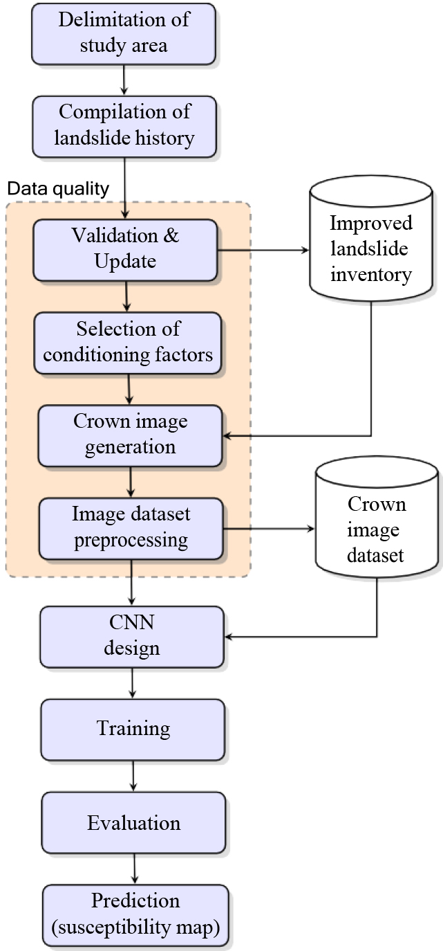

We use a methodology that takes into account the quality of the data and incorporates the landslide crown as the main novelties with respect to related work (Fig. 1). Data quality is fundamental for a good performance of a prediction model, so we carry out the exhaustive validation, correction and updating of the history of landslide events. This task is rarely addressed in other studies, but it is essential when the available information comes from external sources. Our approach considers the geographic position of the landslide crown and the nearest proximity. This new delineation allows capturing the actual conditions that triggered the landslide. Therefore, we have a representation of the phenomenon that is closer to reality and a better accuracy is expected. Typically, related work involves a set of qualitative and quantitative data, whose design, preparation and labeling is a costly task in terms of time and effort. This motivates us to create a dataset composed of images covering only the landslide crown and the surrounding pixels, together with the conditioning factors of the phenomenon. Our solution uses computer vision based on deep learning with a convolutional network, which is currently state-of- the-art tool [37, 38, 39, 40, 41], for a problem that is traditionally treated with classical machine learning.

In the following, we explain in detail these and the other activities that conform the proposed methodology, which is supported by computational tools such as Google Earth, ArcGIS, QGIS, SAGA-GIS, Python programming language and deep learning libraries.

3.1 Delimitation of the geographical area of study

Figure 2.

Geographical location map of the study area.

Landslides occur in large parts of our planet, especially in mountainous areas of highly variable relief and climate [42]. The prediction of these events is becoming a problem of growing interest world-wide. The methodology proposed can be applied to any place or region of the world where landslides are a recurrent phenomenon. We selected the geographical area crossed by the Aloag-Santo Domingo highway (Ecuador), which has been considered in several of our previous studies [25, 26, 27, 28]. This due to the high importance of the phenomenon for the economic and industrial development of the country and the human and material losses it frequently causes.

The highway extends approximately 100 kilometers in the northwestern region of the country, covering the provinces of Pichincha and Santo Domingo (Fig. 2). Its transition from the highlands to the coast gives it great strategic importance. Unlike other related studies [34], our analysis focuses on landslide risk only in the immediate area of influence of the highway, in the form of a corridor, rather than over a vast geographic area. This allows us to obtain a more detailed and accurate understanding of how this phenomenon specifically affects this highway. With the support of GIS, the study area was delimited using the buffer tool, setting a radius of 500 meters on each side to analyze the susceptibility to landslides that directly affect the road and surrounding population.

3.2 Compilation of the landslide history

Figure 3.

Map of the new landslide dataset (manual digitization).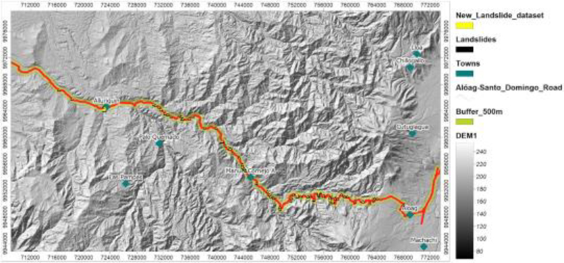

The next step is to know the landslide events that have occurred in the delimited geographical area. What happens in the past can provide clues on what may happen in the future. Compiling a history or inventory of landslide events from scratch can be a more complex process and require more time and resources than requesting government records. We use an inventory provided by the Provincial Autonomous Government (GAD) of Pichincha upon request to access it, which includes the location, date of occurrence, type of mass movement, and photographs of each landslide on the road. A total of 45 landslides were identified from June to September 2014. Although this information derives from an official source, it is necessary to validate, correct possible errors and, most importantly, update the events. One of our main contributions is the creation of a reliable and updated inventory of landslides that have occurred along the Aloag-Santo Domingo highway.

3.3 Validation and update

The available information is transferred to GIS to verify the coordinates of the landslide points with reference to satellite images, discarding those that did not coincide with the place of occurrence of the phenomenon. We updated this inventory with landslide events from 2014 to 2021 through a compendium of information on the date, description, type, and place (kilometer number) of occurrence of the event, mainly from news highlights and videos on social networks. As a physical technical inspection of the site was not possible, a virtual visit was carried out using the digital tool Google Street View, which allowed the extraction of geographical information such as the location in UTM coordinates and the kilometer number of the landslides. The new dataset was digitized from base maps corresponding to the GIS satellite image services.

Figure 3 shows the generated map that including the study area (buffer), the digital elevation model (DEM), existing towns and rivers, as well as the validated landslides from the initial inventory, and the manually digitized polygons of the new places of occurrence of landslides. The final dataset consists of 75 landslides that have not been documented on websites or government sites.

3.4 Landslide conditioning factors

Once the geographical area and the landslide events are known, the most influential conditions for the occurrence of the phenomenon are identified. These variables can be of various types as geological, geomorphological, climatological, vegetation cover, land use, etc. They are called conditioning factors of the phenomenon and can be many and very diverse. The selection of the most appropriate variables is a task for researchers. Numerous conditioning factors have been proposed in the literature. Previous studies corroborate the close relationship between conditioning factors and the occurrence of landslides [2, 9, 18, 43].

Figure 4.

Maps of the conditioning factors automatically generated from the 5-meter resolution DEM.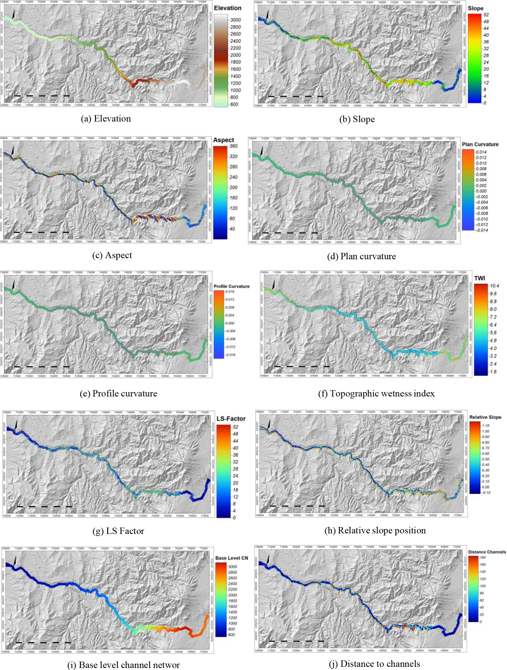

The values of each conditioning factor in the study area are represented by a map from which the CNN input images are extracted [24, 44, 45]. To generate the maps of conditioning factors, a 30-meter resolution DEM of the study area was downloaded from the OpenTopography2 platform. By extracting contour lines and interpolating every 5 meters, a new DEM was obtained with an improved pixel resolution of 5 meters for greater detail using SAGA-GIS. Therefore, all the maps of the variables must have the same pixel resolution. From the new DEM, we can automatically generate 10 maps of different variables through the Basic Terrain Analysis tool (Fig. 4). It is important to note that this DEM, from which the maps of the condi- tioning factors are generated, dates from 2011 and the landslide inventory is from 2014 to 2021, so the information is taken before the landslide event, just as the predictor should be trained.

A group of 14 conditioning factors is selected based on the frequency of appearance in related work, the degree of affectation on the road, and the spatial distribution of landslides [29, 31, 32, 33, 46]. One of the most influential variables is the slope, which is correlated with most of the other variables. It is important to point out the relationship of each conditioning factor with landslides, as well as their behavior in the study area. Elevation or altitude has a direct relationship with relief and slope; strong elevation changes imply steep slopes and instability that contribute to the occurrence of landslides. Elevation increases from 600 m in the west (coast) to 3000 m in the east (highlands) (Fig. 4a). Slope is the inclination of the terrain, so steep slopes are very prone to landslides. The slope ranges from 0 ${}^{\circ}$ to 24 ${}^{\circ}$ in the western and eastern zones, while in the central zone it ranges from 24 ${}^{\circ}$ to 52 ${}^{\circ}$ . The latter being more susceptible to landslides (Fig. 4b). Aspect indicates the orientation of the slope, that is, the direction that the landslide would have along the zone. The values are between 0 ${}^{\circ}$ and 360 ${}^{\circ}$ of azimuth, the western and central zones show opposite directions due to the Pilaton river, while the eastern zone between 120 ${}^{\circ}$ and 360 ${}^{\circ}$ due to steep slopes (Fig. 4c). Plan and profile curvatures are indicators of slope shape, which is viewed from the top and side, respectively. Plan curvature shows values close to zero (linear) in the east and west extremes suggesting lower susceptibility to landslides, while the central zone values are close to $-$ 0.014 (convergence of flow) or 0.014 (divergence) indicating higher susceptibility (Fig. 4d). Profile curvature along the road shows positive and neutral values that accelerate the flow, while negative values decelerate it (Fig. 4e). Topographic wetness index (TWI) identifies possible areas where water accumulates. Relatively high values between 8% and 10% at the extremes of the road (high and low areas), while lower values between 1.5% and 5.6% predominate in the central area due to the water runoff and infiltration process that favors susceptibility to landslides (Fig. 4f). LS factor or erosion index is associated with the loss of soil per unit area on a given slope. More erosion means higher risk, reflected in the mid- dle and eastern central sectors of the road (Fig. 4g). Relative slope position relates the slope to the topography, so it is closely related to the main landslide flow channels. The area most prone to this phenomenon is the Pilaton River, as it is the main drainage channel (Fig. 4h). Vertical distance to a base level of the riverbed establishes the places where landslides can be channeled, that is, the places where the detached material will move. Values below 1800 m are concentrated in the western sector and those above 2400 m in the eastern sector (Fig. 4i). Distance to channels indicates the depth of the water level, which can contribute to the instability of the material and cause landslides. There are distances between 0 m and 180 m. The central-western and central-eastern sectors are more unstable due to the presence of streams resulting from high erosion (Fig. 4j).

Figure 5.

Maps of manually generated conditioning factors.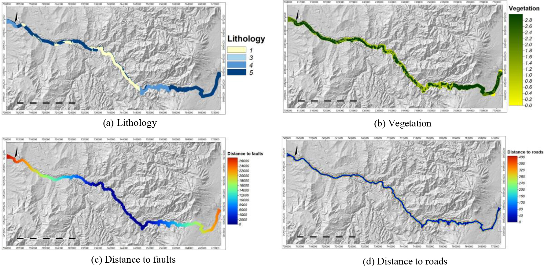

The remaining 4 maps of conditioning factors are generated manually (Fig. 5) from the geological cartography of Quito, Machachi, Las Delicias, and Santo Domingo at 1:100.000 scale, SNI,3 GAD Pichincha, and SIGTIERRAS-MAG.4 Lithology (geology) considers the physical and mechanical properties of rocks, their composition, state, nature, etc., and can determine the instability of slopes. Certain types of lithology are more prone to landslides depending on their conditions. In the study area, there are 4 classes (Fig. 5a): a) andesites, sandstones, and intrusive bodies; b) volcanoclastic sediments and volcanic conglomerates; c) volcanoclastic sediments and undifferentiated terraces; and d) alluvial and colluvial deposits. Vegetation influences the occurrence of landslides. Forests provide stability to the terrain due to the roots that prevent erosion, while anthropic areas and agricultural lands favor it and accelerate landslides. The area shows 3 classes (Fig. 5b): a) forests, b) water bodies and anthropic zone, and c) agricultural lands, shrub and herbaceous vegetation, and other lands. Qualitative values for geology and vegetation must be converted into numerical values for the processing of the prediction model. Following the coding technique known as One-hot encoding, we assign in binary form (values of 0 or 1) the 4 lithology classes and the 3 vegetation classes found in the study area. Distance to roads reflects the impact of anthropic activity and represents the vertical distance of the landslide crowns from the road infrastructure. The degree of affectation may be related to the size and extent of the landslide. There are values between 0 m and 200 m of proximity (Fig. 5d). Finally, distance to faults is the proximity to faults that influence slope breaks and affect not only surface structures but also the permeability of the terrain. The Tandapi (east) and Baba River (west) fault systems are located in the area. They exert structural control over the road, with values between 0 m and 12000 m in landslide zones near the faults and values from 14000 m to 26000 m in zones far from the faults (Fig. 5c). These last two distance variables require the generation of a grid of points with the FishNet tool of ArcGIS; the distance from each landslide crown to the road and the distance from each point to the faults are calculated using the Near tool; the vector layers resulting are joined with the Merge tool and interpolated with the Inverse Distance Weighted (IDW). The generated polygons are then rasterized with the PolygontoRaster tool, which assigned a cell size of 5 meters.

The maps of the conditioning factors or variables of the phenomenon reveal certain values that are closely related to the occurrence of landslides. Our aim is to identify the places with the highest risk and to determine the level of susceptibility along the road.

3.5 Crown image generation

We have a set of maps of the 14 conditioning factors, of which ten are obtained automatically from a DEM of 2011, while the maps corresponding to distance to roads, distance to faults, lithology, and vegetation are produced manually. Due to the 4 qualitative values of lithology, it was necessary to replace them with 4 quantitative variables of binary type, where 1 means the presence of lithology and 0 is its absence. Thus, 4 maps related to lithology are generated. Following the same criteria, vegetation generated 3 maps due to the 3 vegetation values found in the study area. Therefore, a total of 19 maps in raster image format, each image or map is represented as a grid of pixels, where each pixel is a 5-meter square.

This pixel or cell is the mapping unit and its size is a key aspect for analysis and prediction. It corresponds to the interpolation every 5 meter of contour lines from the original DEM. This size is appropriate because the smaller the size, the greater the redundancy; the larger the size, the greater the loss of information. For instance, many cells with the same value of elevation, since in a few meters this value do not change significantly; while a larger size may imply a significant change in this variable with two or more values that cannot be included in a single cell.

Previous studies assumed that each map pixel within the area occupied by the landslide is the value that triggers the phenomenon. This situation is unrealistic, as the extension of a landslide may reach flat areas, even part of the road, where the elevation and slope values are low or null, however, they are taken as positive records of the occurrence of the phenomenon. This undoubtedly distorts the task of relating the occurrence of the landslide and its causes, and the accuracy of the model will decrease under these conditions.

Our proposal is the generation of images covering the starting zone of the landslide as the center and its closest proximity, that is, where the phenomenon originates. The process to identify the crown of the landslide and its associated image consists of the following steps: 1) we manually digitized the shape of each landslide from our updated inventory using ArgGIS and Google Earth satellite imagery as background; 2) the layer of contour lines obtained every 5 meters is superimposed on the previous one; 3) the highest contour level is identified to locate the nearest border of the landslide; 4) we mark on this border the points rep- resenting the crown or origin of the phenomenon. The dimensions of some of the landslides imply that the crowns actually correspond to small areas rather than precise points (Fig. 6); and 5) from the crown of each landslide as the central pixel, we manually generate 5 $\times$ 5 pixel images that store the values that effectively produced the phenomenon for each variable (Fig. 7). These images of 5 $\times$ 5 pixels (1 pixel $=$ 5 meters) would appear small, however, they cover 25 $\times$ 25 meters centered on the landslide crown. Our aim is to capture the conditions that triggered the phenomenon, so larger images would incorporate unnecessary information.

Figure 6.

Landslide crown localization and imaging.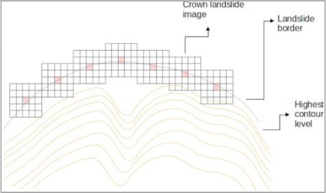

A 5 $\times$ 5-pixel mesh was applied to the DEM-derived images using the Create Fishnet tool. Meshing is important because the limits of the squares coincide with the limits of the pixels in the image. We used this as a base to position the landslide crown to correspond to the central pixel, that is, we digitized each pixel following the limits of the mesh. The procedure was performed manually because the number of images (3 million) exceeded the processing capacity of the computer and ArcGIS.

The treatment given to the other variables is different because the location of the pixels did not match. To solve this problem, the elevation variable raster is converted into points using the Raster to Point tool. For each point generated from the raster (1 point per pixel), the values corresponding to geology, vegetation, distance to faults, and distance to roads are obtained with the Extract Values to points tool. The reverse process was carried out using the Point to Raster tool rasterizing the points with a pixel size of 5 meters so that all pixels have the same spatial location. Subsequently, we use the Clip Raster by Mask Layer tool in QGIS for cropping the images to the desired size of 5 $\times$ 5 pixels. The polygons created manually in ArcGIS that place each landslide crown as the center of a 5 $\times$ 5 pixel image are used as a mask for each variable. Finally, the images are cropped and saved in TIF format in folders with the name of each variable.

3.6 Image dataset preprocessing

Figure 7.

5 $\times$ 5 meter sample landslide crown image (elevation variable).

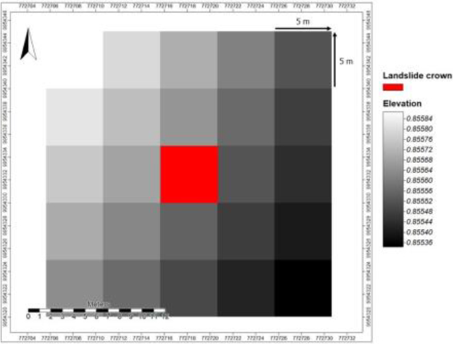
Datasets are key resources in machine learning. Our proposal is to directly use the images representing the landslide crown and variables of the phenomenon. A dataset composed of the images generated in the previous section is the input to train a CNN, which learns the conditions that trigger the phenomenon and obtains a model that predicts the landslide risk. However, it is first necessary to balance, debug, normalize, stack and split the image dataset.

3.6.1 Balance of the dataset

In the learning process, it is recommended to have an equal number of examples of positive and negative landslide occurrences so that the prediction model is free of biases and preferences of any kind. For this reason, nonlandslide images are added to balance the dataset. We identify the areas in which the terrain conditions allow us to ensure a null or almost null probability of the occurrence of the phenomenon. We consider certain criteria such as the slope with values below 10 degrees [47]. Nonlandslide zones are assigned based on the filtering and superposition of the variables with the analysis of frequency histograms, so there is a visual relationship of approximately 1:10 between the values of each variable that favors and avoids landslides. Each nonlandslide point is located in places with very low or no susceptibility to landslide occurrence.

3.6.2 Dataset debugging

Each of the landslides is verified to obtain a quality dataset, with special attention to elevation and slope variables. Inconsistent values of these variables are discarded, for example, slopes less than 10 ${}^{\circ}$ and elevations that do not stand out with respect to the surroundings, as landslides are not commonly found in low and flat areas and may contaminate the dataset. The final result is a total of 262 images, of which 50% correspond to the occurrence of landslides and the other 50% to their absence.

3.6.3 Normalization

Different scales and units of measurement of variables can be a problem training a model. The normalization of the pixels is made with Raster Calculator in QGIS, calculating the maximums and minimums of each quantitative variable. Then, the standardization values between 0 and 1 with MinMaxScaler in Python. For qualitative variables, the one-hot encoding technique is used, which creates new binary columns that indicate the presence or absence of each value within the original data. Thus, these variables are subdivided into 4 geology variables and 3 vegetation variables. Once the normalization is done through the NumPy library, the number of variables increased to 19.

Figure 8.

5 $\times$ 5 $\times$ 19 image stacking.

3.6.4 Image stacking

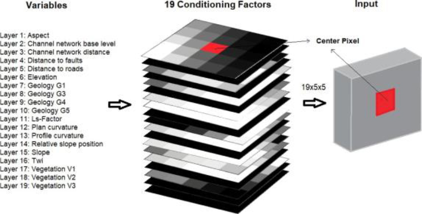
Images processed by a CNN usually contain 1 or 3 channels, corresponding to grayscale or color, respectively. In our case, the images are made up of 19 channels, each associated with a variable. The dstack method from NumPy allows stacking this number of channels in 5 $\times$ 5 $\times$ 19 tensors as shown in Fig. 8. These tensors represent the input images to train the convolutional network.

3.6.5 Dataset split

This operation is classic in machine learning and consists of dividing the dataset into two subsets. The train subset is used to fit the model, while the test subset to evaluate the model performance. A third subset called validation is needed at training time. Based on the proportions recommended in the literature [18, 48], we used a split of 80:20 for training (209 images) and testing (53 images), respectively. For this purpose, the train_test_split function from scikitlearn automatically performs the division in a random way. Furthermore, the training part will be divided into training and validation using cross validation of the data.

Figure 9.

2D convolutional neural network architecture.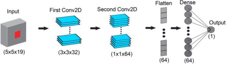

3.6.6 CNN design

Once the dataset was properly prepared for the training process, we design the CNN architecture considering landslide prediction as a binary classification problem, i.e., occurrence or nonoccurrence of the phenomenon. A customized convolutional network that accepts the dimensions of the input image is needed instead of pretrained models, which have image size restrictions and receive conventional 1- or 3-channel color images. The structure of the convolutional network is shown in Fig. 9.

Images of dimensions $w\times h\times c$ , where $w$ is the width in pixels, $h$ the height, and $c$ the number of channels are the input that a CNN processes. About the CNN architecture, our idea is that we did not need a sophisticated architecture since we work with very small 5 $\times$ 5 pixel images due to the local nature of the phenomenon. Thus, we are more interested in convolution operations around the central pixel rather than feature extraction with a very deep network. Only two convolutional layers are needed, due to the small input size. The 5 $\times$ 5 $\times$ 19 images are passed through two 2D convolutional layers, which employ 32 and 64 filters of size 3 $\times$ 3, respectively. These filters are shifted laterally, vertically, and in depth of each image with a padding $=$ valid so that the convolution is applied to the input matrix without going out of its limits. The result is a set of feature maps before applying the activation function tanh. The Flatten layer is responsible for converting these maps into a one-dimensional vector, which is the input of the classifier composed of a dense layer of 64 neurons with the ReLU that connects to a dense output layer of a single neuron with an activation function Sigmoid to provide as output probabilistic values of the occurrence or not of a landslide. A conventional binary classifier is used in the training stage and as a probability estimator in the inference stage.

The number of parameters generated is 28225, which are adjusted during model training. It is worth noting that the model do not use a pooling layer because the aim is not to reduce the size of the image, so we work with the same input dimension of 5 $\times$ 5 pixels. Once the training is completed, a prediction model is obtained to process all the images and produce a landslide probability value (between 0 and 1) for the central pixel of each image. The values generated by the network are imported into a spreadsheet which in turn is imported into a GIS to define the value distribution method, generate the landslide susceptibility classes and visualize the respective map.

4. Experimentation and results

This section describes the experimental part of the project. It focuses on the training of the previously defined CNN processing our image dataset. The model performance is evaluated through learning curves, confusion matrices and accuracy metrics. This allows knowing the suitability of the model for landslide risk prediction and the determination of susceptible areas. The development and execution platform is Google Colaboratory, which is free and offers GPU (Graphics Processing Unit) processing, a large amount of RAM and direct access to data stored in Google Drive or GitHub. The implementation is through programming notebooks using Python and libraries for deep learning such as Keras, Tensorflow, Sklearn and Torch. In addition, OS and Pathlib for folder and file system management, Pandas for data manipulation and analysis, NumPy for data structures and numerical representation of images in tensors, Matplotlib for graph creation and visualization and PIL for image processing.

4.1 Training

The training process starts with the reading of the dataset, which consists of landslide and nonlandslide samples in the same number for image balance. The CNN is trained with all training data (including validation data) and the obtained model is evaluated with the test data. Since our dataset is small, we implement stratified k-fold cross-validation to avoid high variance and increase confidence in the results. This method reduces bias since most of the data is used to train the CNN with different validation subsets. We define k $=$ 5 folds, i.e., the number of subsets into which the training dataset is divided. This means that 5 trainings will be performed instantiating 5 models. Each model is trained on 4 subsets and the remaining subset is used for validation. The StratifiedKFold utility from scikit-learn allows us to generate subsets such that all contain the same percentage of samples for each class, or as close as possible.

Previously, it is necessary to set the hyperparameters that control this process. The loss function is binary crossentropy, 0 for nonlandslide and 1 for landslide, the Adam optimizer with a learning rate of 0.001, and the accuracy metric are established. The image dataset is fed in batches (batch size $=$ 32) into the convolutional network and the model weights are adjusted to reduce the error through a backpropagation process with multiple iterations (epochs) to obtain the desired output. Accuracy and loss values are stored over 100 epochs in a history, which is useful for model performance evaluation. The best model during the training process is saved based on the highest validation accuracy. The weights and architecture of this model are stored in a file with the extension $.h5$ . This to use it later in the predictions. In addition, the value of the learning rate automatically decreases to a given minimum if there is no improvement in the loss of validation.

Figure 10.

Learning curves of each training and validation of the 5-fold method. Accuracy (left) and loss (right).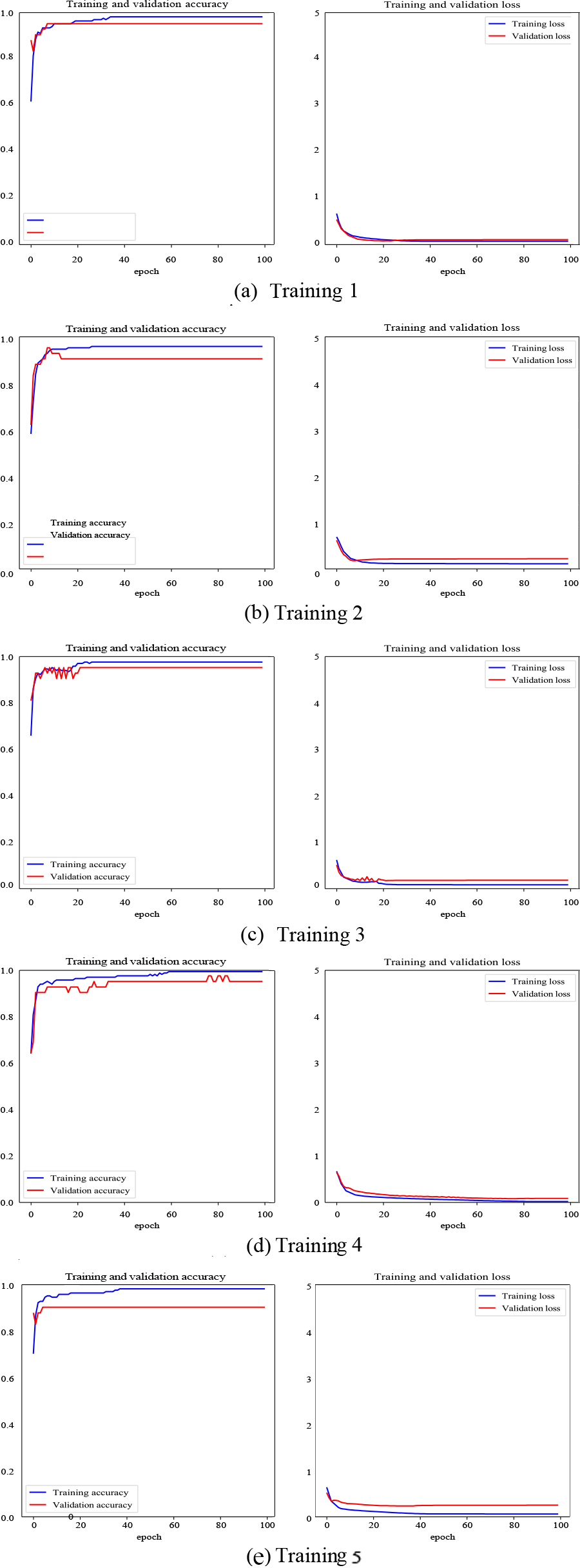

Table 2

Accuracy and loss in the test subset for each model. Mean and standard deviation are included

Metric	Model 1	Model 2	Model 3	Model 4	Model 5	Mean	Std. dev.
Accuracy	0.9434	0.9434	0.9811	0.9057	0.9623	0.9472	0.0279
Loss	0.3623	0.2122	0.1016	0.5958	0.2739	0.3092	0.1862

Figure 11.

Central region of the highway used for landslide prediction.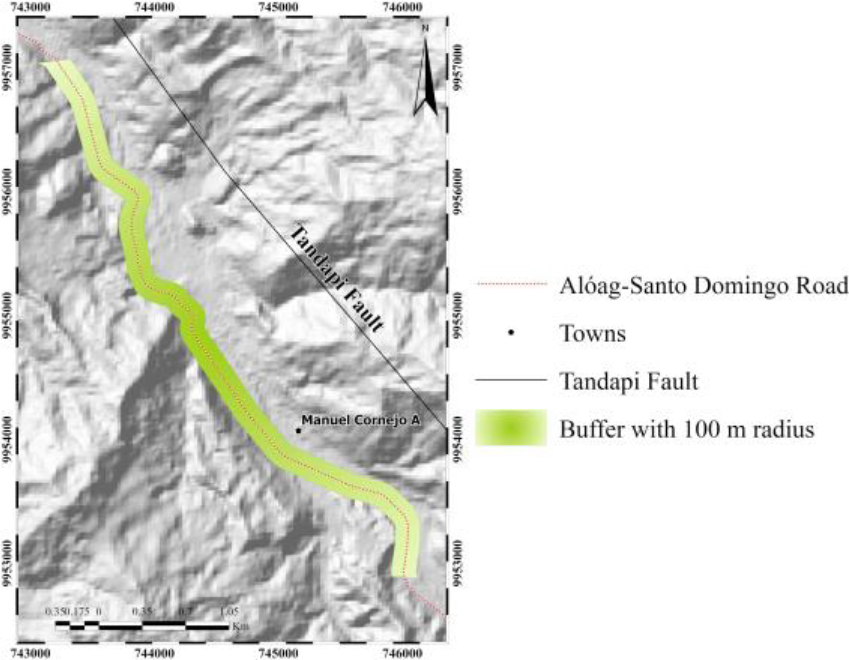

The different runs allow us to detect the variability in the performance and generalization ability of the model. To know how the model behaves during training and validation, visual tools such as learning curves are used. The Matplotlib library allows to plot the accuracy and loss values stored in the history, both in the training and validation stages. The training results of the 5 models are shown in Fig. 10.

The performance of the five models is quite satisfactory. The accuracy curves in both the training and validation phases increase as the epochs progress and remain stable at a high percentage of accuracy. Moreover, these curves is very close to each other, evidencing that there is no overfitting. For the loss or error curves, the behavior is similar, but in the opposite direction. There is a marked trend to zero for both curves.

4.2 Evaluation

Evaluation must be performed on the test data, which is the data not seen during the training stage. For this purpose, the accuracy metric is calculated using the same test subset in each training. The final evaluation performance of k runs is averaged as the overall model performance. In addition, we provide the mean and standard deviation of the accuracy of the k runs used for k-fold cross-validation.

Table 2 summarizes the evaluation performed on the test data. The arithmetic mean of the five runs (94.72%) is reported as the final measure of the accuracy of our model. This measure is considered more robust to the problem that different divisions of the data can lead to different results. The standard deviation (0.0279) is small, reflecting a low variability of the precision values obtained from the 5 evaluations. We also include the loss values, which are in the range between 0 and 1, suggesting acceptable behavior.

Since we use a different dataset, architecture and geographic area than other landslide-related studies, our contribution is novel and it is not possible to directly compare the current work with others. Experimental results show an average accuracy of 94.72%, which becomes the state of the art performance for the specific dataset developed and geographical area considered.

5. Landslide susceptibility map

We have proved five models that are acceptable, however, the best one (98.11% accuracy) is selected to predict the occurrence of landslides and generate the susceptibility map of the Aloag-Santo Domingo highway. The prediction is made for each of the pixels of the study area. We must consider that the model receives input images of 5 $\times$ 5 pixels to provide as a response a value between 0 and 1, which is the probability of a landslide for the central pixel. Next, we explain the procedure for the generation of the 5 $\times$ 5 pixel images.

Figure 12.

Workflow for generating the landslide susceptibility map.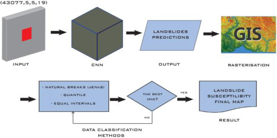

Figure 13.

A sample of the predictions file exported to GIS.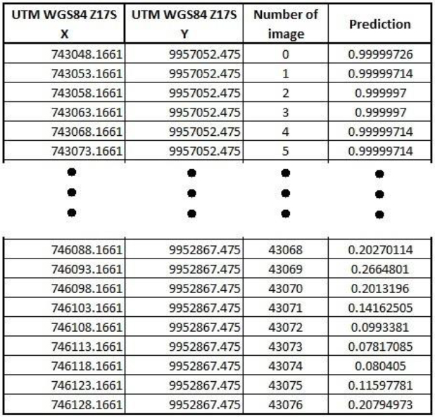

The elevation raster is converted to points using ArcGIS and resulting an equal spacing grid in which each point is located in the center of each pixel. The buffer operation is applied from each point as a center to generate circles of 12.5 m radius, which are then transformed into 25 $\times$ 25 m (5 $\times$ 5 pixels) squares. These squares must be cropped to obtain the images required by the prediction model. Cropping all the images is too time-consuming, so we focused only on the central part of the road, as this region has the highest recurrence rate of landslides covering 100 meters on each side of the road and a distance of approximately 5.5 km (Fig. 11). The new geographical area for the prediction of the susceptibility to landslides contains 43077 squares of 5 $\times$ 5 pixels and is superimposed on the complete image of the study area for each of the 19 layers corresponding to our variables, resulting a total of 818463 images. These images form the dataset for the prediction of the CNN model, which generates the probability values to create the map of landslide susceptibility on the highway.

Figure 14.

Landslide susceptibility map.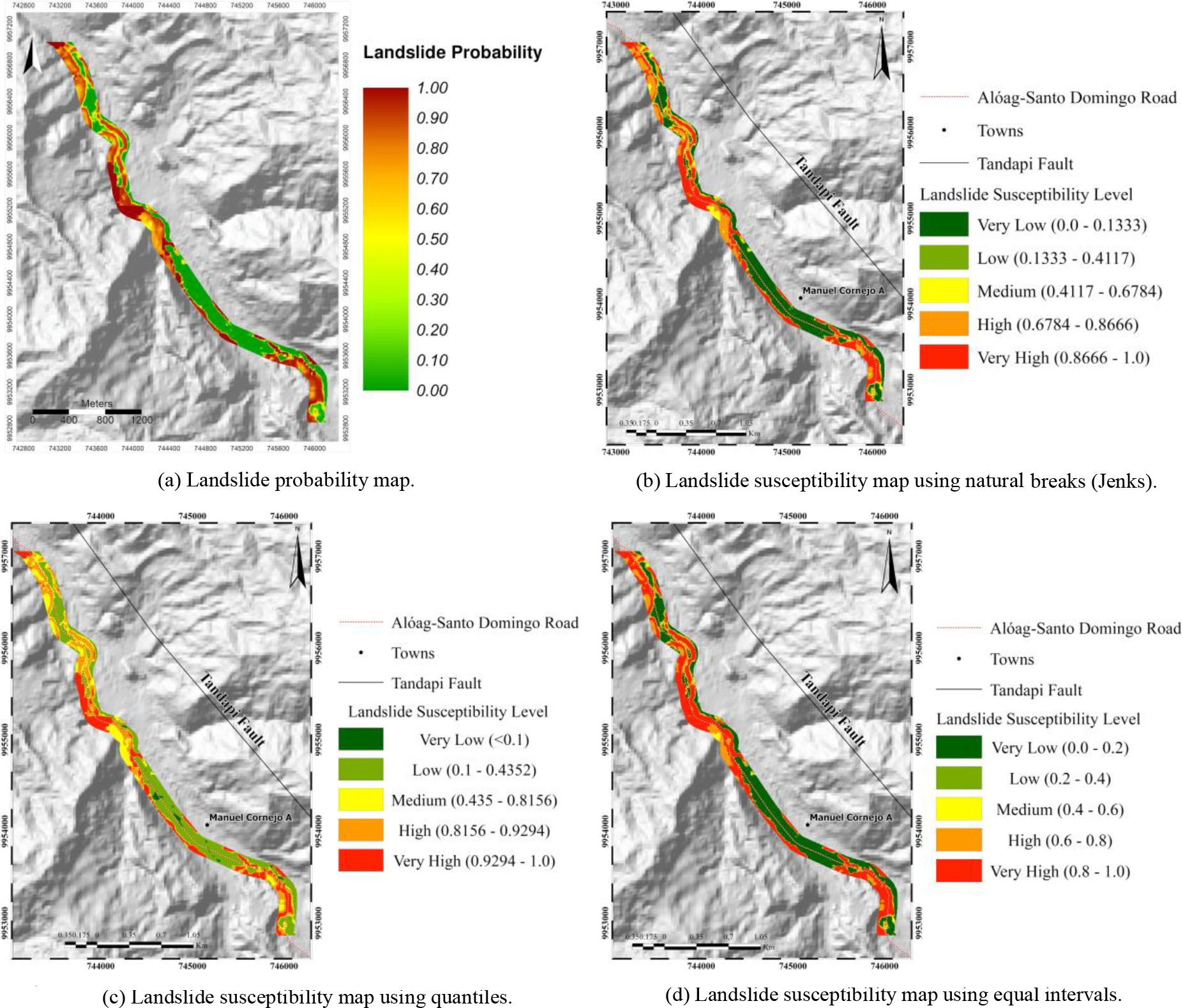

Images are organized and stored in folders, each of which corresponds to each conditioning factor. An important aspect is the nomenclature used to name the images and facilitate stacking them prior to prediction. This name is constituted by the raster of the variable followed by the position in numerical order and the file format, for example, Aspect_105.tif, Elevation_105.tif, Slope_105.tif, etc. First, they are sorted alphabetically so that all the tensors of each image contain the same conditioning factor. Then we generate empty tensors of dimensions (43077,5,5) using NumPy to store 43077 input images of 5 $\times$ 5 pixels for each conditioning factor. Iteratively, all image files are read, transformed into arrays and stored in the tensors. The 5 $\times$ 5 $\times$ 19 images are stacked iteratively and stored in a tensor of dimensions (43077,5,5,19), i.e., the number of images covering the study area, the width, the height, and the number of channels (variables) required by the CNN model. By loading the model file saved in h5 format, the prediction is performed to generate the landslide probability values that are stored in an array of dimensions (43077,1).

The landslide susceptibility map is generated following the procedure illustrated in Fig. 12.

The probability values obtained from the prediction are exported by means of a Pandas data frame to GIS together with the image number, the predicted value and the geographic location of the central pixel in UTM coordinates (WGS84-17S). Figure 13 shows an extract with the header and tail of this list of values. The determination of the coordinates of the central pixel is simple because the polygon number used for clipping (generated by the buffer) corresponds to the same as the image plus one, that is, if the image number is 50, the polygon number is 51, so that by calculating the coordinates of the centroid of the polygon, we know to which central pixel it corresponds.

The data file is imported into a GIS and converted into a colored raster with values between 0 and 1, representing the probability of landslide of the central area of the highway (Fig. 14a). However, it is necessary to distribute the probability values in classes associated with different susceptibility levels. There are several methods for the distribution of values, each with characteristics that can better reflect reality. We analyze which is the most convenient for our case among the following ones: Natural Breaks (Jenks), Quantiles, and Equal intervals.

Natural Breaks minimize the mean deviation between values of the same class and maximize the mean deviation between classes, that is, intervals are defined in places where there are relatively large jumps between one class and another [49, 50, 51]. Quantiles allow each class contains the same proportion of values, the classification is adapted to classes that have a good linear distribution; however, it is a somewhat misleading method since low values can be included within classes with high values [52]. Equal intervals divide the range of attribute values into classes of equal size, which is useful when it is desired to emphasize the amount of value of an attribute in relation to the other values [52].

It is possible to choose one of these methods in ArcGIS as well as the number of risk categories, ranging from very low, low, medium, high to very high susceptibility. Once the three maps have been generated, we make a visual comparison to select the most appropriate one. Based on the landslide inventory, all maps provide a high level of confidence because areas with a higher concentration of landslides have a higher susceptibility [53]. However, the map generated by the quantile method (Fig. 14c) is quite similar to the map of landslide probability values without classification. This is not suitable for representing well-defined zones and levels of landslide susceptibility. The Jenks and Equal Intervals maps (Fig. 14b and 14d, respectively) are very similar and show a closer representation of what may occur in reality. There are slight differences between both maps, but the Jenks method presents a better visualization where all classes are clearly visible. In particular, we are interested in higher variability of values from different classes (interclass variability) and lower variability of values from the same class (intraclass similarity). This is exactly how the natural breaks method works.

6. Conclusions

We have used CNN-based deep learning to perform landslide risk prediction and the generation of a susceptibility map of the area of interest. The visual and accuracy results indicate that this solution is a comparable alternative to classical ML methods. The performance of a learning model depends on the quality of the data, so one of our main tasks was to improve the dataset needed for landslide risk prediction. By using previous geological and fieldwork information provided by a governmental entity, we validated and updated the historical record on landslides through journalistic sources and satellite image interpretation. We provide a more reliable and up-to-date landslide inventory that is the basis for generating an image dataset that represents each conditioning factor of the phenomenon. These images 5 $\times$ 5 pixels of resolution correspond to the crown of the landslide, since we focus exclusively on the place where the phenomenon starts, unlike other works that consider the area covered by a landslide, which can be very extensive including values that do not actually cause the phenomenon. Therefore, we handle the values that effectively produce the landslide, achieving a representation of the data that is closer to reality. This helps to better capture important patterns about the relationship between conditioning factors and landslide occurrence. Consequently, the convolutional network model is able to generate better predictions of the landslide susceptibility of the area. The CNN model used for the study of the Aloag-Santo Domingo highway achieves an average in its three runs of 97.48% accuracy without evidence of overfitting. These results suggest that the use of CNN for the prediction of landslide risk from images of conditioning variables is highly effective like the use of conventional classifiers. As a result of the model prediction, we obtain a susceptibility map created with a GIS. By contrasting the landslide crowns used to train the model and the areas of high susceptibility on the map, we can see that they are in the same place, which increases the confidence in the results obtained. The selected 14 conditioning factors (19 variables) are considered relevant for this work taking account the related-literature; however, we identified the slope, elevation, geology, and distance to faults as the outstanding factors. The latter is considered a triggering variable because the area is located between two major fault systems (Baba river and Tandapi). Therefore, the construction of linear infrastructure (roads) should always be perpendicular to the faults, never parallel, as in the case of the Aloag-Santo Domingo highway.

7. Future work

The landslide susceptibility map must be made for the entire study area. This requires processing a quantity of 3 million 5 $\times$ 5 pixel images, which could be handled in batches, as shown here, or in its totality with high computational power. This will allow the competent authorities to take the appropriate measures to avoid material and, above all, human losses. Our work can be complemented by involving meteorological factors such as precipitation, temperature, humidity, among others. These variables are not considered in this work because data from weather stations in the area are very limited and scarce. We believe that sufficient information on these variables, mainly precipitation, can improve the accuracy of the landslide prediction model and the identification of susceptible areas. We suggest classifying the type of landslide to obtain more detailed results on the type of phenomenon that can occur on the road.

Footnotes

github.com/jfcepeda97/DATASET_DESLIZAMIENTOS_Via-Aloag_Santo_Domingo.git.

https://opentopography.org/.

https://sni.gob.ec/coberturas.

http://geoportal.agricultura.gob.ec/index.php/visor-geo.

References

Alcántara Ayala

. Landslides: deslizamientos o movimientos del terreno? Definición, clasificaciones y terminología. Investigaciones Geográficas. 2000; 7-25.

Zhu

Huang

Fan

Huang

Chen

Zhang

Wang

. Landslide Susceptibility Prediction Modeling Based on Remote Sensing and a Novel Deep Learning Algorithm of a Cascade-Parallel Recurrent Neural Network. Sensors. 2020; 20(6). doi: 10.3390/s20061576. https//www.mdpi.com/1424-8220/20/6/1576.

Suárez

. Nomenclatura y clasificación de movimientos. Deslizamientos: Análisis Geotécnico. 1998; 37. https//www.academia.edu/29057579/Nomenclatura_y_Clasificaci%C3%B3n_de_los_Movimientos.

Valencia

JEG

. Propuesta metodológica basada en un análisis multicriterio para la identificación de zonas de amenaza por deslizamientos e inundaciones. Revista Ingenierías Universidad de Medellín. 2006; 5(8): 59-70.

Vásconez Urbano

Jibaja Urbano

. Análisis multicriterio dentro de un SIG para la identificación de zonas susceptibles a deslizamientos, en la parroquia San José del Tambo, cantón Chillanes, provincia Bolívar. B.S. Tesis, Universidad Estatal de Bolívar Facultad de Ciencias de la Salud. 2020.

Liu

. Geological disaster recognition on optical remote sensing images using deep learning. Procedia Computer Science. 2016; 91: 566-575.

Kuradusenge

Kumaran

Zennaro

. Rainfall-induced landslide prediction using machine learning models: The case of Ngororero District, Rwanda. International Journal of Environmental Research and Public Health. 2020; 17(11): 4147.

Wang

Zhang

Yin

Luo

. Landslide identification using machine learning. Geoscience Frontiers. 2021; 12(1): 351-364. doi: 10.1016/j.gsf.2020.02.012. https//www.sciencedirect.com/science/article/pii/S1674987120300542.

Liu

Z-Q

Guo

Lacasse

J-H

Yang

Choi

. Algorithms for intelligent prediction of landslide displacements. Journal of Zhejiang University-SCIENCE A. 2020; 21: 412-429. doi: 10.1631/jzus.A2000005.

10.

Wang

Fang

Hong

. Comparison of convolutional neural networks for landslide susceptibility mapping in Yanshan County, China. Science of The Total Environment. 2019; 666: 975-993.

11.

Wehle

H-D

. Machine Learning, Deep Learning, and AI: What’s the Difference? (2017).

12.

Ngeljaratan

Moustafa

Pekcan

. A compressive sensing method for processing and improving visionbased target-tracking signals for structural health monitoring. Computer-Aided Civil and Infrastructure Engineering. 2021; 36(9): 1203-1223.

13.

Lara-Benítez

Carranza-García

Riquelme

. An experimental review on deep learning architectures for time series forecasting. International Journal of Neural Systems. 2021; 31(3): 2130001.

14.

Hussain

Chen

Zheng

Shoaib

Shah

Ali

Afzal

. Landslide susceptibility mapping using machine learning algorithm validated by persistent scatterer In-SAR technique. Sensors. 2022; 22(9): 3119.

15.

Sajedi

Liang

. Uncertainty-assisted deep vision structural health monitoring. Computer-Aided Civil and Infrastructure Engineering. 2021; 36(2): 126-142.

16.

Tian

Zhang

Jiang

Zhang

Duan

. Noncontact cable force estimation with unmanned aerial vehicle and computer vision. Computer-Aided Civil and Infrastructure Engineering. 2021; 36(1): 73-88.

17.

Palacios Orejuela

. Susceptibilidad a deslizamientos en la vía Alóag-Santo Domingo, mediante Lógica Difusa. Revista Geoespacial. 2020; 17: 1-12. doi: 10.24133/geoespacial.v17i2.1571.

18.

Fang

Wang

Peng

Hong

. Integration of convolutional neural network and conventional machine learning classifiers for landslide susceptibility mapping. Computers & Geosciences. 2020; 139: 104470. doi: 10.1016/j.cageo.2020.104470.

19.

Benamara

Val-Calvo

Alvarez-Sanchez

Diaz-Morcillo

Ferrandez-Vicente

Fernandez-Jover

Stambouli

. Real-time facial expression recognition using smoothed deep neural network ensemble. Integrated Computer-Aided Engineering. 2021; 28(1): 97-111.

20.

Macias-Garcia

Galeana-Perez

Medrano-Hermosillo

Bayro-Corrochano

. Multi-stage deep learning perception system for mobile robots. Integrated Computer-Aided Engineering. 2021; 28(2): 191-205.

21.

Gasienica-Jozkowy

Knapik

Cyganek

. An ensemble deep learning method with optimized weights for drone-based water rescue and surveillance. Integrated Computer-Aided Engineering. 2021; 28(3): 221-235.

22.

Martins

Papa

Adeli

. Deep learning techniques for recommender systems based on collaborative filtering. Expert Systems. 2020; 37(6): 12647.

23.

Hassanpour

Moradikia

Adeli

Khayami

Shamsi-nejadbabaki

. A novel end-to-end deep learning scheme for classifying multi-class motor imagery electroencephalography signals. Expert Systems. 2019; 36(6): 12494.

24.

Küçükogğlu

Rueckauer

Ahmad

de Ruyter van Steveninck

Güçlü

van Gerven

. Optimization of neuroprosthetic vision via end-to-end deep reinforcement learning. bioRxiv. 2022; 2022-02.

25.

Rodriguez

Meneses

Garcia-Rodriguez

. Improving landslides prediction: meteorological data preprocessing using random forest-based feature selection. In International Workshop on Soft Computing Models in Industrial and Environmental Applications (pp. 379-387), (2021a), Springer.

26.

Rodriguez

Salvador-Meneses

Garcia-Rodriguez

. Predicting landslides with machine learning methods using temporal sequences of meteorological data. In International Workshop on Soft Computing Models in Industrial and Environmental Applications (pp. 348-357), (2021b), Springer.

27.

Guerrero-Rodriguez

Garcia-Rodriguez

Salvador

Mejia-Escobar

Bonifaz

Gallardo

. Defining High Risk Landslide Areas Using Machine Learning. In International Work-Conference on the Interplay Between Natural and Artificial Computation (pp. 183-192), (2022a), Springer.

28.

Guerrero-Rodriguez

Garcia-Rodriguez

Salvador

Mejia-Escobar

Bonifaz

Gallardo

. Landslide Prediction with Machine Learning and Time Windows. In International Work-Conference on the Interplay Between Natural and Artificial Computation (pp. 193-202), (2022b), Springer.

29.

Shibao

Zhuang

Jiaqi

Jia

Jiewei

Jie

Yuting

. Evaluation of Landslide Susceptibility of the Ya’an-Linzhi Section of the Sichuan-Tibet Railway based on Deep Learning, 2021. doi: 10.21203/rs.3.rs-714294/v1.

30.

Prakash

Manconi

Loew

. A new strategy to map landslides with a generalized convolutional neural network. Scientific Reports. 2021; 11. doi: 10.1038/s41598-021-89015-8.

31.

Habumugisha

Chen

Rahman

Islam

Ahmad

Elbeltagi

Sharma

Liza

Dewan

. Landslide Susceptibility Mapping with Deep Learning Algorithms. Sustainability. 2022; 14(3). doi: 10.3390/su14031734. https//www.mdpi.com/2071-1050/14/3/1734.

32.

Ghasemian

Shahabi

Shirzadi

Al-Ansari

Jaafari

Kress

Geertsema

Renoud

Ahmad

. A robust deep-learning model for landslide susceptibility mapping: A case study of Kurdistan Province, Iran. Sensors. 2022; 22(4): 1573.

33.

Youssef

Pradhan

Dikshit

Al-Katheri

Matar

Mahdi

. Landslide susceptibility mapping using CNN-1D and 2D deep learning algorithms: comparison of their performance at Asir Region, KSA. Bulletin of Engineering Geology and the Environment. 2022; 81(4): 1-22.

34.

Zhang

Wang

Chen

Sun

Luo

Han

. Evaluation of different machine learning models and novel deep learning-based algorithm for landslide susceptibility mapping. Geoscience Letters. 2022; 9(1): 1-16.

35.

Bui

T-A

Lee

P-J

Lum

K-Y

Loh

Tan

. Deep learning for landslide recognition in satellite architecture. IEEE Access. 2020; 8: 143665-143678.

36.

Mora

Vahrson

Mora

. Mapa de Amenaza de Deslizamientos, Valle Central, Costa Rica. Centro de Coordinación para la prevención de desastres naturales en América Central (CEPREDENAC), 1992.

37.

Hou

Samaras

Kurc

Gao

Davis

Saltz

. Patch-based convolutional neural network for whole slide tissue image classification. In Proceedings of the IEEE conference on computer vision and pattern recognition (pp. 2424-2433), 2016.

38.

Gómez-Silva

de la Escalera

Armingol

. Back-propagation of the Mahalanobis istance through a deep triplet learning model for person Re-Identification. Integrated Computer-Aided Engineering. 2021; 28(3), 277-294.

39.

Demertzis

Iliadis

Pimenidis

. Geo-AI to aid disaster response by memory-augmented deep reservoir computing. Integrated Computer-Aided Engineering. 2021; 28(4): 383-398.

40.

Nogay

Adeli

. Detection of epileptic seizure using pretrained deep convolutional neural network and transfer learning. European neurology. 2020; 83(6): 602-614.

41.

Nogay

Adeli

. Diagnostic of autism spectrum disorder based on structural brain MRI images using, grid search optimization, and convolutional neural networks. Biomedical Signal Processing and Control. 2023; 79: 104234.

42.

Cruz-Roa

Basavanhally

González

Gilmore

Feldman

Ganesan

Shih

Tomaszewski

Madabhushi

. Automatic detection of invasive ductal carcinoma in whole slide images with convolutional neural networks. In Medical Imaging 2014: Digital Pathology (Vol. 9041, p. 904103). SPIE, 2014.

43.

Dao

Jaafari

Bayat

Mafi-Gholami

Moayedi

Phong

H-B

T-T

Trinh

Luu

Quoc

Thanh

Pham

. A spatially explicit deep learning neural network model for the prediction of landslide susceptibility. CATENA. 2020; 188: 104451. doi: 10.1016/j.catena.2019.104451. https//www.sciencedirect.com/science/article/pii/S0341816219305934.

44.

Zhang

Lin

. Computer-vision-based differential remeshing for updating the geometry of finite element model. Computer-Aided Civil and Infrastructure Engineering. 2022; 37(2): 185-203.

45.

Choi

Sohn

. Real-time structural displacement esti-mation by fusing asynchronous acceleration and computer vision measurements. Computer-Aided Civil and Infrastructure Engineering. 2022; 37(6): 688-703.

46.

Azarafza

Akgün

Atkinson

Derakhshani

. Deep learning-based landslide susceptibility mapping. Scientific Reports. 2021; 11(1): 1-16.

47.

Vázquez

Domínguez-Cuesta

. Identificación de zonas susceptibles a deslizamientos en Tegucigalpa, Honduras. Limitaciones del modelo del talud infinito. Geogaceta. 2021; 69: 51-54.

48.

Bustos

Estrada

Soria

Mejia-Escobar

. Estimación del Riesgo de Deslizamientos Mediante Algoritmos de Aprendizaje Automático (Vía Calacalí-Nanegalito). https://1fa1iz5erxtlacejtwzzqw.on.drv.tw/www.myhomepage.com/.

49.

Chen

Yang

Zhang

. Research on Geographical Environment Unit Division Based on the Method of Natural Breaks (Jenks). ISPRS – International Archives of the Photogrammetry, Remote Sensing and Spatial Information Sciences. 2013; XL-4/W3, 47-50. doi: 10.5194/isprsarchives-XL-4-W3-47-2013.

50.

North

. A Method for Implementing a Statistically Significant Number of Data Classes in the Jenks Algorithm (Vol. 1, pp. 35-38), 2009. doi: 10.1109/FSKD.2009.319.

51.

Lin

. A Comparison Study on Natural and Head/tail Breaks Involving Digital Elevation Model, 2013. https//www.diva-portal.org/smash/get/diva2:658963/FULLTEXT02.pdf.

52.

Osaragi

. Classification methods for spatial data representation. Osaragi, Toshihiro (2002) Classification methods for spatial data representation. Working paper. CASA Working Papers (40). Centre for Advanced Spatial Analysis (UCL), London, UK, 2008.

53.

Zhao

Chen

. Optimization of Computational Intelligence Models for Landslide Susceptibility Evaluation. Remote Sensing. 2020; 12: 2180. doi: 10.3390/rs12142180.

Improving landslide prediction by computer vision and deep learning

Abstract

Keywords

1. Introduction

2. Related work

Table 1 Work collected and aspects considered in the review of the literature

3.4 Landslide conditioning factors

3.6.2 Dataset debugging

3.6.3 Normalization

3.6.5 Dataset split

4. Experimentation and results

4.1 Training

5. Landslide susceptibility map

7. Future work

Footnotes

References

Table 1
Work collected and aspects considered in the review of the literature