Sage Journals: Discover world-class research

Abstract

This article summarizes principles and ideas from the emerging area of applying conditional computation methods to the design of neural networks. In particular, we focus on neural networks that can dynamically activate or de-activate parts of their computational graph conditionally on their input. Examples include the dynamic selection of, e.g., input tokens, layers (or sets of layers), and sub-modules inside each layer (e.g., channels in a convolutional filter). We first provide a general formalism to describe these techniques in an uniform way. Then, we introduce three notable implementations of these principles: mixture-of-experts (MoEs) networks, token selection mechanisms, and early-exit neural networks. The paper aims to provide a tutorial-like introduction to this growing field. To this end, we analyze the benefits of these modular designs in terms of efficiency, explainability, and transfer learning, with a focus on emerging applicative areas ranging from automated scientific discovery to semantic communication.

Keywords

Conditional computation neural networks modularity explainability efficiency

1 Introduction

In the last twenty years, neural networks (NNs) have undergone two opposing trends. On one hand, the number of practical applications has continued to grow, fueled by successes in, among others, language modeling [37], drug design [93], rendering, and language-vision reasoning [64]. On the other hand, their design has crystallized around a very small set of layers (e.g., multi-head attention) and principles (e.g., permutation equivariance), while the focus has shifted on scaling up their training, both in terms of data and parameters [37]. Apart from scale, maybe less than a dozen components and variations thereof are enough to categorize the vast majority of neural networks deployed nowadays.

Among these design principles, sequentiality has remained a key component. NNs, be they convolutional, recurrent, or transformers, are composed of a stack of differentiable operations, which are activated in sequence for each input to be processed. Stated in another way, their computational graph, i.e., the sequence of primitive operations executed on the underlying hardware, is fixed beforehand when instantiating them. Because NNs have continued to scale in depth and width, this has led to several issues in terms of computational performance and efficiency [22]. Standard techniques to make NNs more efficient only address this partially, by replacing the original network with other static models having fewer layers (distillation [95], pruning [42]), less precision per parameter, or by approximating each weight matrix (e.g., via low-rank factorization).

By viewing neural networks as computing systems, this behavior is counter-intuitive. Hardware components are designed based on their expected peak usage, while only executing a fraction of their resources at any given time (e.g., memory). Similarly, software libraries and operating systems are composed of millions of lines of code, only a handful of which are selected and run in a given moment, thanks to the use of branches, loops, and conditional execution. Recently, a large body of literature has flourished on embedding similar sparse modularity principles in the design of neural networks [67]. Based on the original idea of conditional computation [5], this has blossomed into a large number of practical implementations, ranging from mixture-of-experts (MoEs) [85] to dynamic mechanisms to select tokens and layers in transformers [52]. This tutorial is intended as an organized, uniform overview and entry point into this growing body of literature.

The benefits of developing networks that can dynamically adjust their computational graph go beyond memory or time efficiency. More and more, neural networks are treated in the same way as software [40], and deploying them requires the possibility of quickly debugging their predictions [11], continually fine-tuning them on new data, and transferring parts of their knowledge from one network to the other [3], similarly to standalone software libraries. As we will see, dynamically-activated neural networks provide a principled way to improve both zero-shot transfer and generalization [70] (Section 4.2) and explainability of the models (Section 4.3). This aligns with the requirements of many novel applications of NNs, from scientific discovery [93] to AI-native telecommunications [86, 99]. In particular, smart semantic communication networks [86] envisioned in the so-called beyond 6G model necessitate networks that can flexibly adapt to bandwidth and energy constraints, while ensuring transferability and communication through separate neural modules.

For the purpose of this tutorial, we consider three flavors of dynamism: (a) neural components that can restrict their computation to a smaller subset of input tokens (dynamic input sparsity); (b) layers that can selectively activate sub-components for processing a token (dynamic width sparsity); and (c) layers that can be completely skipped during their execution (dynamic depth sparsity). As we show in Section 2, a simple mathematical formalism encompasses all three cases. Section 2 also highlights how modularity can be achieved with the addition of a small set of primitives to our networks’ toolkit, namely, the possibility of sampling in a differentiable way elements from a set. We discuss in Section 2.2 the simplest technique to this end, the Gumbel-Softmax trick [35, 50], and some common extensions.

We then proceed to discuss three notable implementations of these concepts in Section 3: early-exit (EE) models, mixture-of-expert (MoE) layers, and token selection mechanisms. While these models are generally discussed in separate fashions (e.g., see [51, 82] for EEs, and [20, 105] for MoEs), viewing them as specific instances of a general framework highlights many similar trends and characteristics. In fact, we argue that designing networks with dynamically activated components is not simply a matter of enhancing performance: in all these cases, the resulting networks are more apt at adapting to variable system’s constraints (e.g., decreased energy usage), specialization, catastrophic forgetting, and multimodality. We build on these insights in Sections 4 and 5, where we list potential research directions for these models including adapting their computational cost and energy at inference and training time in an elastic way, zero-shot transfer, robustness, and explainability.

Relation to prior works: we do not claim to be the first to discuss these ideas, nor to present them in a general way. We simply hope to provide a simple, cohesive entry point into an extremely fascinating and growing research direction in the literature. Recently, modular deep learning [67] has been proposed as a general term for neural networks where computation is functionally decomposed into units that are sparsely activated. Compared to [67], our formalism is simpler and we focus on a smaller set of ideas: for example, we do not consider input composition methods, nor soft routing strategies, and we focus on viewing modularity as discrete sampling inside neural networks. Hence, we provide an orthogonal view to [67], to which we refer for a broader outlook on modularity and composition. We also focus on a tutorial exposition, preferring simplicity and clarity to completeness. We only describe the simplest techniques for differentiable sampling, and we refer to [59] for a larger and more in-depth introduction to this field. Additional entry points in the literature include [24] (for an overview up to 2021 of dynamism in NNs) and [22] for designing faster and more efficient transformer models.

2 Three types of conditional computation

2.1 A general formalism for sparse modularity

Neural networks can be described as the composition of several trainable, differentiable operations of the form: $y = f (x, w)$ (1) where x denotes the input, w the module’s parameters, and f the specific operation. Because of functional composition, f can represent an operation at any level of complexity, e.g., a basic linear algebra operation, a layer (convolutional, recurrent,...), or a composite block, such as the classical combination of token mixing, channel mixing, and layer normalization operations found in transformers.

Most of our discussion focuses on transformer-like architectures, where the input is composed of a set of tokens, representing parts of the complete input [78] (e.g., subwords in a sentence or patches in an image). The input x in (1) is purposefully left vague: depending on the scenario and the layer, x can be a single token (e.g., for the fully-connected blocks inside a transformer), the entire set of tokens, a mini-batch of inputs, or other forms of data aggregation.

We are interested in augmenting (1) to allow the dependence of the different quantities to vary based on some conditioning inputx_c, where x_c can be equal to x, some linear or non-linear projection of x (in order to decouple the conditioning input from the input used for the layer and increase the flexibility of the dynamic mechanism), or some additional input information (e.g., a latent token representing the language of the speaker in an audio model [47]).

Suppose we have available some trainable subsampling operation, defined over the conditioning input x_c and over some set $S$ , such that: $Γ (S, x_{c}) \subseteq S .$ (2) Practically, sets are always represented in some matrix format inside neural networks (e.g., by stacking all elements row-wise), in which case we assume the relevant quantities in (2) to follow the same conventions. As an example, if $S$ is represented by a matrix S, (2) can be implemented by row-wise masking of the corresponding elements: $Γ (S, x_{c}) = M ⊙ S$ (3) where M is a binary mask of suitable shape with rows set to either 0 or 1. Different implementations can be obtained depending on whether the size of the output mask is known in advance (e.g., how many tokens to keep in a given layer), or must be estimated by Γ itself. We will see later on in Section 2.2 how such an operation can be implemented in practice.

This small addition allows us to implement several levels of modularity inside our neural network. First, assume the input x can be decomposed into smaller components x ={ x₁, …, x_n }. In many cases, this is a natural decomposition, e.g., tokens inside a transformer, time instants for a sequence, or frames for a video input. However, they can also correspond to additional register tokens [18], to elements extracted from some external memory (e.g., AdaTape [101]), or additional views or modalities. Then, dynamic input sparsity (Fig. 1) is achieved by combining the layer with a subsampling operation on the input:

Fig. 1

Input sparsity: A differentiable mechanism subsamples input tokens to be processed by the later parts of the network (we show original image patches in the figure, but the tokens can be equivalently be replaced by their latent representations if we consider an intermediate layer of the architecture).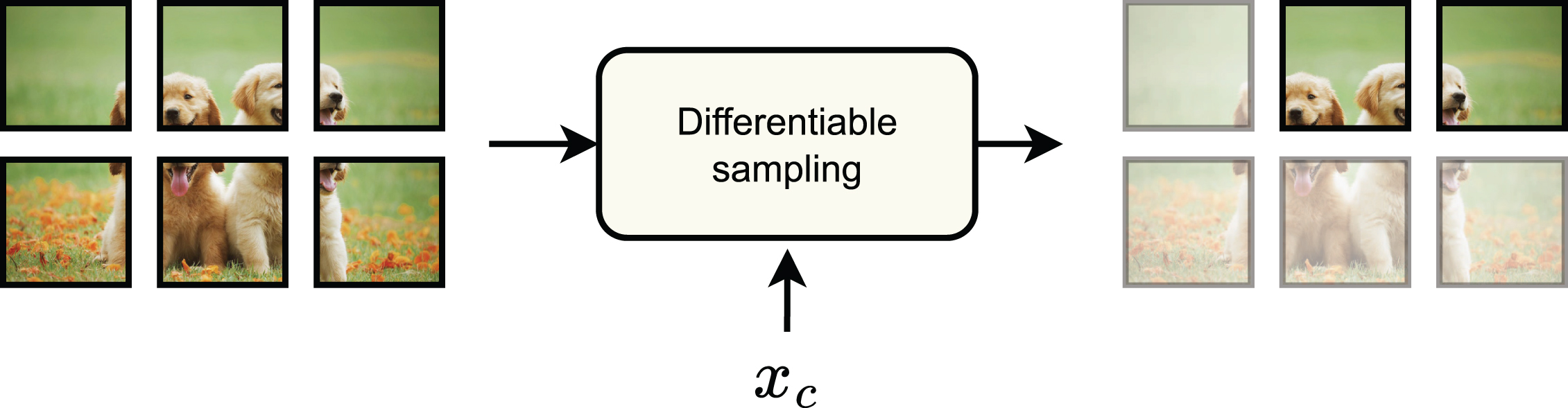

Input sparsity : f (Γ (x, x_{c}), w)

(4) This allows the layer to focus exclusively on input components that are relevant to the current operation. As an example, consider an image with a very wide, uniformly blue background: for the majority of tasks, we can imagine the layer to be able to operate even when removing the vast majority of tokens corresponding to such background [96]. This is, indeed, observed in practice, as we’ll describe in Section 3.5.

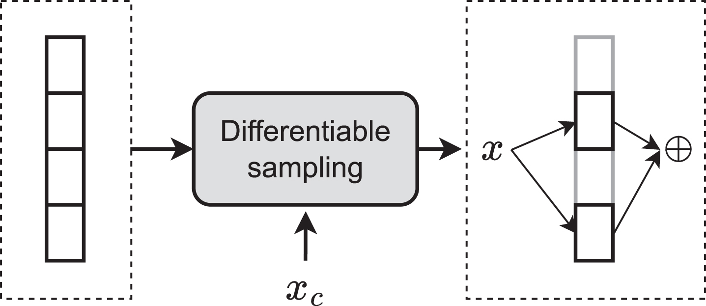
Second, assume the weights themselves can be decomposed into blocks b ={ w₁, …, w_m }, and the entire function decomposed as: $f (x, w) = \oplus ({f_{1} (x, w_{1}), \dots, f_{m} (x, w_{m})}),$ (5) where ⊕ is a permutation equivariant operation that aggregates the results of the different blocks. This is also a very natural decomposition in practice: for example, f_i could correspond to a single output channel in a convolutive layer, with ⊕ being a concatenation. Or, f_i can be a head in a multi-head attention layer, with ⊕ being a concatenation followed by a projection. In this case, what we call dynamic width sparsity (Fig. 2) can be achieved by subsampling the blocks:

Fig. 2

Width sparsity: Different parts of a layer (e.g., experts) can be activated based on the conditioning value.

$\begin{matrix} Width sparsity : f (x, Γ (w, x_{c})) = \\ \oplus (Γ ({f_{1} (x, w_{1}), \dots, f_{m} (x, w_{m}), x_{c}}) \end{matrix}$ (6) Imposing some form of structure over w is fundamental since subsampling each weight separately would result in a highly unstructured form of dynamic pruning, which is generally very difficult to optimize and control [36]. Once again, this formulation is very generic: for example, if each f_i corresponds to an activation function, subsampling with cardinality 1 corresponds to choosing the best activation function for each token or each input, in a form of dynamic model selection mechanism [48]. If each f_i is an entire model, this can be used to route information across blocks with different types or complexity (see, e.g., layer stitching [61]). We will see in Section 3.2 a common implementation of this principle in the context of MoEs, and defer more general discussions to Section 4.

Third, even if a weight decomposition is unavailable, dynamic computation can still be achieved by considering the entire layer as a single block and conditionally skipping its execution. This dynamic depth sparsity (Fig. 3) can be achieved easily by rewriting the layer with an additional, untrainable scalar weight σ = 1, and writing:

Fig. 3

Depth sparsity: A subset of the layers can be deactivated by the sampling mechanism, like in early-exit networks.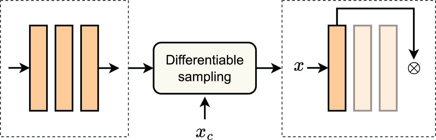

Depth sparsity : f^{'} (x, w, Γ ({σ}, x_{c})) =

(7)

σ (x_{c}) f (x, w) + (1 - σ (x_{c})) x

(8) where we assume the empty set ∅ to be implemented as 0 in practice. As a variant of this idea, we can skip entire blocks of layers by exiting the network instead of adding a skip connection in (8). We will see concrete implementations of this concept in Section 3.1.

2.2 Discrete sampling: the Gumbel-Softmax trick

Before proceeding, we discuss briefly the implementation of the subsampling layer Γ. As a prototypical example, we restrict our analysis to subsampling a single element from the set in input. In this case, a very common implementation is the so-called Gumbel-Softmax (GS) trick [35], also known as the concrete distribution [50]. In this section, we only provide a high-level overview, and we refer to [34] for a fuller exposition.

First of all, we process the inputs with some trainable layer $p (S, x) \in ℝ^{| S |}$ to provide a real-valued score for each element in $S$ , which is proportional to its probability of being sampled. In this section, we drop the subscript from the conditioning input x_c for readability. The implementation of p depends on the use case. For example, suppose that the conditioning input is a tensor $x \in ℝ^{h \times w \times d}$ coming from intermediate output of a CNN having width w, height h, and d channels, while $S$ is the set of output channels in a convolutive layer, of which we want to select a single one [31]. We associate to each channel a trainable vector c_i, and compute an affinity score via the dot product with a pooled representation of the image [31]: $v = MLP (\sum_{i, j} x_{ij})$ (9) $p (S, x) = [v^{⊤} c_{1}, \dots, v^{⊤} c_{| S |}]$ (10) Many other designs for p are possible based on x and $S$ . Let us denote by p the output of p, and by g_i samples from the so-called Gumbel distribution [35]. We also assume that the elements of $S$ correspond to integers, $S = {1, \dots, | S |}$ , in which case we simply write $Γ_{| S |} (x)$ for the subsampling over the set of integers. Then, the following operation provides an unbiased sample from $S$ , with the probability of sampling the i-th element $p (s \in S) \propto exp (p_{s})$ proportional to p_s: $s = \underset{i}{arg max} {p_{i} + g_{i}} .$ (11) Removing the Gumbel noise g_i corresponds to taking the element with the highest score p_i, while sampling provides a degree of freedom that is helpful in exploring possible alternatives. Since the probabilities p_i are implicitly trained via $p (S, x)$ , the network can learn to select the element from $S$ which is most useful for the specific input x. In the case of channel selection, for example, this can lead to specializing single channels to specific types of inputs.

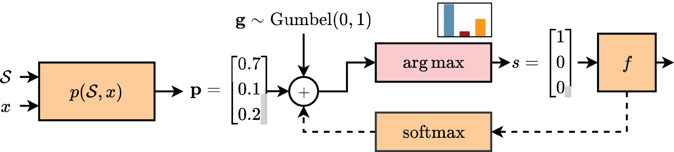
The operation in (11) is not easily trainable via gradient descent (since its gradient will be zero almost everywhere), but it can be relaxed with a softmax approximation: $s_{i} = \frac{exp ((p_{i} + g_{i}) / τ)}{\sum_{j} exp ((p_{j} + g_{j}) / τ)} .$ (12) The quality of the approximation can be controlled by the user-defined parameter τ, sometimes called the temperature [34]. The values in s are not binary anymore, being generic convex combinations of the (one-hot) representations from the elements in $S$ . However, a common relaxation is to use the binary values in (11) during the forward pass of the network, and relax the gradients to use the soft approximation in (12) during the backward pass. This is called straight-through estimation (STE). A high-level overview of the complete schema is given in Fig. 4.

Fig. 4

Overview of the Gumbel-Softmax trick. We show in orange differentiable operations (the argmax’s gradient being zero almost everywhere) and with a dashed arrow the relaxed backward path.

The GS trick can be easily extended to sampling more than a single value by replacing the arg max with a top-k operation [43]. Suitable generalizations, such as the entmax family [16], can also sample binary vectors with a variable number of elements. The simplicity of the GS trick makes it widespread in many applications, but several other types of sampling layers can be found in the literature, especially for more complex combinatorial spaces, for which we refer to [59]. A larger overview of possible sampling operations for MoE layers is also given in Section 3.3.

3 Concrete implementations

The previous section has introduced a generic framework for designing networks with dynamic computational graphs. In the literature, these ideas have coalesced around a few, notable set of implementations. In this section we overview three of the most popular ones: early exits (Section 3.1), MoE layers (Section 3.1), and token sampling (Section 3.5) as examples of networks having dynamic depth, width and input, respectively. In all cases we focus on the key strengths and drawbacks of each approach, highlighting how they connect to the framework of Section 2.

3.1 Early exits

Early exit neural networks (EENNs) were introduced based on the idea that not all the inputs to a network are required to go through all the layers of the model to be correctly classified [89]. In fact, the accuracy of a network can decrease with respect to the depth on particularly easy samples, a phenomenon known as overthinking [80].

Consider a neural network (sometimes called the backbone network in this context), which can be either trained from scratch or pre-trained. In an early-exit framework, the backbone is augmented with auxiliary classifiers (early exits) which are connected at intermediate outputs of the backbone. These auxiliary blocks can be trained all at the same time or in a layer-wise fashion [82], while at inference time they are used to halt the computation when the model is confident enough about the prediction. This is an example of dynamic depth sparsity (Section 2), except that an entire subset of layers is skipped at the same time.

We introduce first the most common formulation of EENNs, in which early exits are jointly trained while the early exit logic is defined manually with additional hyper-parameters. As already stated, we can see a neural network as a composition of b sequential blocks: $f (x) = f_{b} \circ f_{b - 1} \circ \dots \circ f_{1} (x)$ (13) where ∘ denotes function composition, b is the last layer of the backbone, and we remove the dependency on the parameters for simplicity. Where to place the auxiliary classifiers is in general a hyper-parameter [82], but here, for clarity, we add a classifier after each block, producing multiple prediction functions: $y_{i} (x) = c_{i} \circ (f_{i} \circ f_{i - 1} \circ \dots \circ f_{1} (x))$ (14) where c_i is a small classifier (e.g., for a CNN, a typical design is to have a global average pooling operation followed by a fully-connected layer, while for a transformer we can apply a fully-connected layer on a specialized class token). This formulation leads to an EENN which is capable of classifying input samples at any stage of the computation through the sequence y₁ (x) , y₂ (x) , …, y_b-1 (x) , f (x). Ideally, each classifier can specialize on a subset of the training samples based on the complexity of the input. In the simplest case, given a desired output y, all early exits can be trained simultaneously by minimizing the sum of the losses for each classifier: $L = α CE (y, f (x)) + \sum_{i = 1}^{b - 1} β_{i} CE (y, y_{i} (x)),$ (15) where CE is the cross-entropy loss, and α, β₁, …, β_b-1 are hyper-parameters that balance the loss contribution from each early exit. At inference time, an exit can be chosen by comparing, e.g., the predicted class probability or the entropy of the prediction to a user-defined parameter acting as a threshold. Other strategies include combining predictions based on trainable [81] or geometric [97] ensembling.

These networks have found applications in many fields recently. Concerning NLP, many strategies with BERT have been proposed [98 , 114], varying from patience-based EE [111] to extra classification layers [98]. For computer vision, EE applications vary based on the strategy, including multi-exiting [4 , 95], and loss-weight adjustment [94]. Also, the tasks vary, spanning semantic segmentation [44], video recognition [23], adversarial training [41], and image compression [99]. Recently, EE strategies have been proposed also for vision-language models [88].

Although this formulation of EENNs (or minor variations thereof) is very common in the literature (see e.g., [8 , 111]), it only fits partially our view of dynamic sparsity, since the computational graph is unchanged during training and the dynamism is only obtained via an external heuristic. To this end, [81] proposed a mechanism to optimize the early exit selection during training, called differentiable branching. Suppose we augment each early exit with an additional output that we denote as γ_i (x). The key idea of differentiable branching is to define a new recursive output, which is given by a soft composition of the original outputs: ${\tilde{y}}_{i} (x) = γ_{i} (x) y_{i} (x) + (1 - γ_{i} (x)) {\tilde{y}}_{i + 1} (x)$ (16) where the recursion stops at i = b, where γ_i (x) =1 by definition. At inference time, this can be turned into an early exit module by viewing γ_i (x) as a binary classifier and thresholding it at 0.5. By replacing the gates γ_i (x) with samples from a GS distribution, we return to the general setting described in Section 2. In fact, if the outputs of γ_i (x) are binary we canidentify: $Γ_{b - 1} (x) = [\begin{matrix} γ_{1} (x) \\ (1 - γ_{1} (x)) γ_{2} (x) \\ ⋮ \\ [\prod_{i = 1}^{b - 2} (1 - γ_{i} (x))] γ_{b - 1} (x) \end{matrix}]$ (17) with the subsampling block over the indexes of the early exits. This can also be given a Bayesian interpretation under the stick-breaking process [69]. While the sampler in (17) is conditioned on the full input, other choices are possible. For example, in multitask learning a separate task embedding can be used to select different exits for different tasks [107], while in the case of transformers, only the class token can be used to decide an optimal exit strategy [30]. Being able to train the choice of early exit is fundamental because it allows us to regularize it further for, e.g., better inference-accuracy trade-offs: we revisit this idea in Section 4.1. See [51, 81] for in-depth reviews on EENNs and [81] for a fuller description of differentiable branching.

3.2 Mixture-of-experts

Mixture-of-Experts (MoEs) models were introduced more than thirty years ago as adaptive algorithms to perform dynamic ensembles of individual machine learning algorithms, denoted as experts in that context [105]. Recently, MoE layers in neural networks have gained popularity, especially for LLMs and large vision modules [78]. They allow scaling the model’s parameters while keeping the compute budget constant, and they offer the possibility of distributing the training by decomposing the computation of a layer over multiple GPUs [78]. As a side product, they offer dynamic width sparsity by selectively activating only parts of the layer for each input. At the time of writing, the largest open source language and vision models are based on a MoE formulation [17 , 78].

In a MoE layer, the trainable parameters are grouped into topologically identical blocks called experts. In the forward pass, a decision block (called router in this context) selects a subset of expert blocks (typically, only a fixed number of k experts, with k selected beforehand, is chosen) that will be activated and routes the input data to the selected experts. More formally, the MoE layer can expressed as: $f (x, w) = \sum_{i = 1}^{n} γ_{i} (x) f_{i} (x, w_{i})$ (18) where γ is the routing function and f₁, f₂ … f_n are the experts. In its simplest form, this is a sparse linear combination of the outputs of the experts. This is immediately seen to be an instance of 6 with Γ_n (x) = [γ₁ (x) , γ₂ (x) , …, γ_n (x)], provided that the outputs of γ_i (x) are sparse.

The unique advantage of MoEs is that only a fraction of the network parameters, depending on the chosen value for k, are used for computation. Such fraction can be tuned by changing the value of k. Additionally, one can devise routing functions such that experts focus on different areas of the input space, leading to specialized sub-networks (see Section 4.2 for a discussion on specialization and Section 3.3 for an overview of routing algorithms for MoE layers).

As stated earlier, the seminal idea of MoEs dates back to [39], where this paradigm is regarded as an ensembling technique with soft gates. The first work that adopts MoEs in a modern deep learning scenario is [84]. Here, the gate becomes sparse, i.e., a fixed top-k operation and the main goal is scaling the number of parameters. Based on these initial results, in the past few years, the deep learning community witnessed a steep growth of MoE’s success in conjunction with transformer architectures.

Unlike early exiting, where the routing function typically works at the level of input samples (e.g., images for a CNN), an MoE layer as in (18) can work at the level of individual tokens in a transformer. More specifically, in the fully-connected layers of a transformer block, each token can be assigned to one or more experts. Transformer MoEs have been proposed for NLP [21, 72], for vision [78] and even for multimodal training [58]. Additional variants can be applied to individual heads of an attention block [108] or adapters in a fine-tuning context [106].

3.3 Routing in mixture of experts

Different routing strategies can be adopted to orchestrate the experts. These are defined in the gating function γ and usually leverage some differentiable sampling method similar to the Gumbel-Softmax trick (Section 2.2). Routing is a crucial aspect of any MoE architecture, as it must perform a matching between input data and expert network, conditioned on the input data itself. Decisions taken by the routing function govern the training. They can determine faster convergence and expert specialization or cause expert starvation, a peculiar situation where only a few experts are always activated due to their ever-increasing expertise.

The routing algorithm usually adopts a dot product for computing similarity between the embedding of each routed sample (e.g. a token in a transformer) and n trainable expert embeddings (one for each expert). Once this operation has occurred, the assignment can happen according to various methods.

In top-k token choice, each token is assigned to the k most similar experts, where k is an arbitrary value. This is the original approach from [84], and it usually requires additional regularization to avoid expert starvation and training instability. The same approach has been adopted with minor changes (e.g. balancing loss and the k factor) in [21, 74]. Top-k expert choice, proposed in [112], tries to solve the expert balancing problem by assigning each expert to the k most similar tokens, where k is an arbitrary value. Other works [15, 79] cast the expert assignment problem into a reinforcement learning framework and train over a routing policy to assign each token to a single expert. Finally, [115] achieves surprisingly good results by randomly assigning experts to routed samples. An empirical comparison of different routing functions can be found in [49], while a broader overview of MoE layers is given in [20].

3.4 Soft routing

We discuss here a variant of the MoE layer in (18), known as soft MoE, which has become popular recently to avoid training instabilities in the layer. The key idea is to use the gating function to combine the layer’s inputs [71] or weights [57] instead of the model’s outputs. These variants also provide a fixed compute budget which is decoupled from the total number of parameters, but they are generally easier to implement and train.

First, denote by x₁, …, x_n the tokens in input to the layer. The first soft MoE variant we consider can be defined as [71]: $f_{i} (x, w_{i}) = f_{i} (\sum_{i = 1}^{n} γ_{i} (x_{i}) x_{i}, w_{i})$ (19) i.e., each expert is activated with a soft combination of input tokens. Compared with standard top-k routing, each expert is only activated once in this formulation, irrespective of the number of tokens. The output of the layer for a single token is then given by another soft combination, this time over the experts’ outputs: $f (x_{i}) = \sum_{i = 1}^{n} γ_{i} (x_{i}) f_{i} (x, w_{i})$ (20) By comparison, another soft MoE variant can be achieved by performing a soft combination of the experts’ weights [57]. Denote by f (x, w) the generic architecture of a single expert, we have: $f (x) = f (x, \sum_{i = 1}^{n} γ_{i} (x) w_{i})$ (21)

A thorough comparison of the relative benefits of hard vs. soft routing is still lacking in the literature, but we highlight a few benefits in Section 4.

3.5 Token dropping and token merging

We conclude with a brief analysis of token selection mechanisms. In particular, we consider two cases of token selection, which we refer to as token dropping (removal of tokens from the model) and token merging (combination of tokens). Both are conditional computation techniques that can be employed in any transformer model. The fundamental idea behind token dropping and token merging is that the input data often contains information that is nearly useless for the final task. Since transformers operate on set-based inputs with no fixed cardinality, one can dynamically reduce the number of tokens being passed to each layer depending on the relevance of said tokens for the final task.

More formally, let X be the set of n tokens inside a transformer model stacked horizontally. For the purpose of this section, the subsampling operation Γ can be implemented as a matrix multiplication of the input matrix X and a mask M: $X^{'} = Γ_{n} (X) = M X$ (22) Depending on the properties of the matrix M, we can obtain either token dropping or token merging:

Token dropping: M is a matrix of shape n′ × n that selects a subset of n′ elements from the original tokens. This can be achieved by setting each row to a one-hot vector.

Token merging: M is a binary matrix of shape n′ × n, with the requirement that each column sum to one. In this way, the output tokens are combinations of the input ones, so each input token participates in a single output token. This can be seen as a dynamic variant of the standard pooling used in CNNs.

Both methods aim to reduce the computational cost of the forward pass of a transformer by reducing the number of tokens. The mask M is usually computed depending on the input data, M = MLP (X), in such a way as to eliminate only redundant information, such as background patches in an image. This is usually done either by small modules that are added to the backbone model [76] or by evaluating some channels added to the tokens for this purpose [52]. For token selection, when dealing with mini-batches of inputs, the sub-sampling operation in (22) cannot be performed easily in a vectorized way. In these cases, (22) can be replaced by a masking operation as in (2), with the additional constraint that subsequent selection modules can only select values that were not masked previously [76]. In these cases, performance gain only materialize at inference time, while at training time most operations are still executed in a masked way.

Token dropping and token merging have been largely explored in recent years; some of the most impactful works on these topics in the field of vision transformers are [52, 76] for token dropping, while [9, 62] explored token merging. These techniques have also been employed in other fields where transformers are predominant: in 3D computer vision token dropping has been applied to point cloud transformers by [103], while in NLP [32] applied token dropping in the pre-training of BERT, obtaining significant speedups.

4 Research directions

Designing neural networks with sparse modularity principles has a number of benefits. The first and most studied is increased efficiency, both in training and in inference (Section 4.1). However, modular networks show emergent properties also in terms of specialization and transferability (Section 4.2), as long as providing a blueprint for a new type of explainability techniques (Section 4.3). We briefly overview these aspects in the following sections.

4.1 Efficiency in training and inference

Conditional computation has gained significant attention for accelerating training and inference in deep learning models [22, 67]. Often, the time saving comes with a drop in accuracy, making it important to assess the accuracy/computation trade-off. An interesting example is shown in Fig. 5. The approaches can vary based on several factors. For example, some research investigated the sparsification of CNNs [91] and of transformers [12, 36], some others focused on some specific aspects of the net, such as the gradients [19], the backpropagation, the activations [13] and the attention layers [14, 90]. For clarity, we focus here, mainly, on efficiency aspects related to the three families of models seen in Section 3, focusing on emerging trends and open challenges. To make the analysis more timely and precise, we have reported all the methods analyzed in Table 1.

Fig. 5

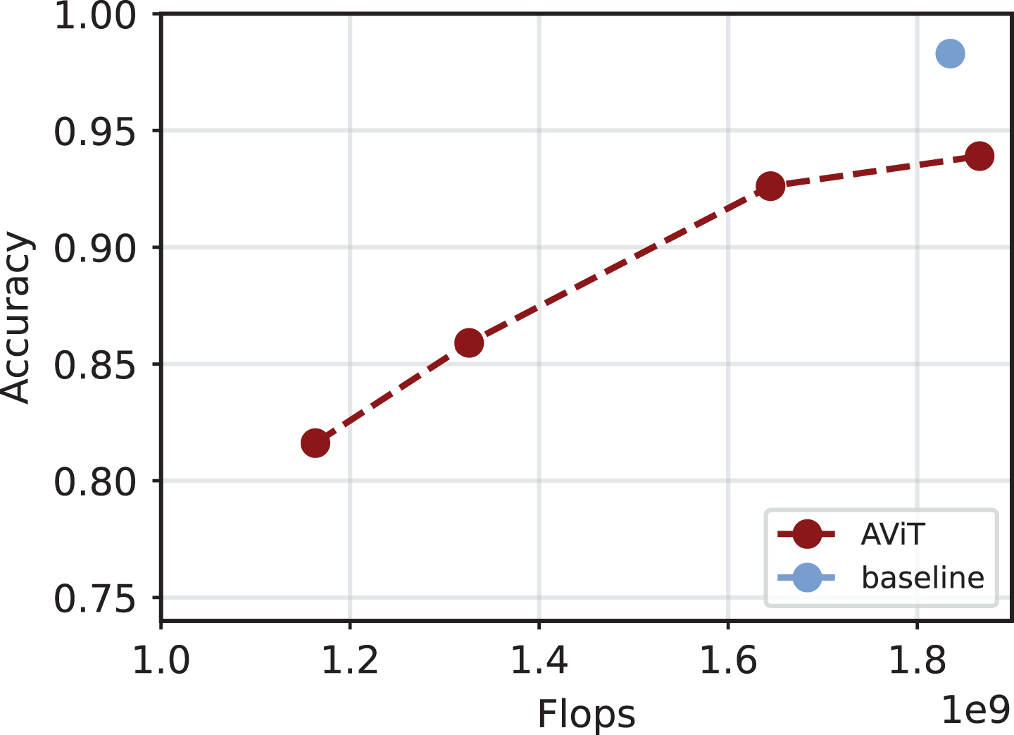
Example of accuracy-flops trade-off for inference with A-ViT [104]. Specifically, the architecture is a DeiT, trained on Imagenette.

Table 1

Overview of methods to improve efficiency of the models, including baseline algorithms not discussed in the text (e.g., pruning)

Method	Approach	Additional parameters	Pre-training	Reduce latency	Reduce FLOPs/MACs
Dynamic convolutions [91] (2020)	Sparsity	Yes	-	Yes	Yes
Scaling transformers [36] (2021)	Sparsity	-	-	Yes	-
SViTE [12] (2021)	Pruning	-	-	Yes	Yes
Sparse momentum [19] (2019)	Pruning	-	-	Yes	Yes
SparseViT [13] (2023)	Pruning	Yes	-	Yes	Yes
Sparse transformers [14] (2019)	Factorization	Yes	-	-	Yes
Differentiable branching [81] (2020)	Early exits	Yes	-	Yes	Yes
Adaptive early exits [8] (2017)	Early exits	Yes	-	Yes	-
L2W-DEN [25] (2022)	Early exits	Yes	-	Yes	-
PABEE [111] (2020)	Early exits	Yes	-	Yes	-
Branchynet [89] (2016)	Early exits	Yes	-	Yes	-
AEP [80] (2023)	Early exits	Yes	-	Yes	Yes
BoF [63] (2020)	Early exits	Yes	-	-	Yes
DeepSpeed-MoE [74] (2022)	MoE	Yes	Yes	Yes	Yes
Sparsely-gated MoE [84] (2017)	MoE	Yes	-	-	Yes
V-MoE [78] (2021)	MoE	Yes	-	-	Yes
MoA [108] (2022)	MoE	Yes	-	-	Yes
SUT [87] (2023)	MoE	Yes	-	-	Yes
MoV/MoLoRA [106] (2023)	MoE	Yes	Yes	-	Yes
EMoE [73] (2023)	MoE	-	Yes	-	Yes
GMoE [46] (2022)	MoE	Yes	Yes	-	Yes
MoEfication [109]	MoE	Yes	Yes	-	Yes
SADMoE [68] (2023)	MoE	Yes	Yes	-	-
A-ViT [104] (2022)	Token sampling	-	-	Yes	Yes
ToMe [9, 10] (2022)	Token sampling	Yes	-	Yes	Yes
AdaViT [52] (2022)	Token sampling	Yes	-	-	Yes
DynamicViT [76] (2021)	Token sampling	Yes	-	Yes	Yes
MSViT [28] (2023)	Token sampling	Yes	-	Yes	Yes
GTP-ViT [100] (2024)	Token sampling	Yes	-	Yes	Yes
Colt5 [1] (2023)	MoE	Yes	Yes	Yes	Yes
PatchMerger [77] (2022)	Token sampling	Yes	Yes	Yes	Yes
ToFu [42] (2024)	Token sampling	-	Yes	Yes	Yes
ACM [96] (2023)	MoE/Token sampling	Yes	Yes	-	Yes

When training from scratch an EENN, the joint training described in Section 3.1 cannot provide faster training since all exits must be trained simultaneously. Soft combinations of the early exits [81] combined with sampling tricks could be useful, but this aspect has been scarcely explored in the literature, possibly due to training instabilities and collapse. Still, EEs can provide indirect benefits to training by accelerating the convergence of deep neural networks [8, 89]. They can also improve the inference efficiency of large-scale pre-trained models [25, 111], making them more discriminative [89], act as a regularization technique [80], and possibly reduce training problems (e.g. vanishing gradient phenomena) [63]. In addition, they can be trained in a layerwise fashion if one starts from a pre-trained network [24]. In Table 1, we can see that most of these methods require additional parameters, leading to a latency reduction.

Compared to EEs, MoEs were investigated mostly to speed up training by distributing the experts across different GPUs [20], or to accelerate inference by activating a subset of experts for each forward pass. For the former, tiling the model across separate machines requires customized implementations [74]. In addition, to achieve an effective stable throughput, training must avoid collapses of the routing function, and care must be taken to balance the number of tokens that are sent to the different experts. This last point can be achieved with the addition of so-called balancing losses, e.g., batch prioritized routing [15 , 78]. Due to these problems, open-source implementations of large MoE models have generally lagged behind proprietary models, with some preliminary steps being taken in this direction [102], as observable also in Table 1.

The benefits of applying MoEs can also vary depending on the specific component that is being replaced. In [84], MoEs replace MLP layers to scale-up transformers. A similar methodology, for vision, was presented in [78]. Other approaches proposed to replace attention layers [108], entire blocks [87] of the net, and adapters [106]. By comparison, soft MoEs (Section 3.4) can reach similar gains as standard MoE layers while being simpler to train. Finally, the majority of MoEs are trained from scratch, but recently moefication has emerged as an interesting research direction, in which a pre-trained model is converted to an MoE variant by clustering the activations [73, 109] (see Table 1 to see the approaches based on pre-training). These variants provide different accuracy-time trade-offs based on the specific routing function. Additional emerging research trends are exploring dynamic variants of routing to provide a flexible inference budget instead [68, 96].

Finally, reducing the number of tokens with token selection techniques is a straightforward strategy to improve the inference time of the network. Most methods in this sense have focused on token dropping [9 , 104]: A-ViT adopts a token halting approach (shown also in Fig. 5); AdaViT [52] proposes a light-weight decision network, attached to the backbone to produce decisions on-the-fly; DynamicViT [76] proposes an attention-masking strategy to block interaction of redundant tokens; MSViT [28] proposes a conditional gating mechanism that selects the token scale for every image region; GTP-ViT [100] introduces a Graph-based Token Propagation (GTP) to propagate the information of less significant tokens. During training, token selection is generally achieved by masking the corresponding input elements (Section 3.5). Designing token selection mechanisms that can improve training time (for a fixed compute budget) is still an open challenge.

Some works have focused more on specific tasks, such as diffusion [10], long-input sequences [1], or to better understand the general pattern of token dropping [27]. For token merging, PatchMerger [77] proposes a module that reduces the number of tokens by merging them between two consecutive intermediate layers [77]. Recently, a hybrid solution, Token Fusion (ToFu) [42], proposed to put together the benefits of both token pruning and token merging. Token selection can also be combined with the other methods discussed in this paper. As an example, Adaptive Computation Module (ACM) [96] is a technique that combines token dropping with a dynamic width principle, in which each token is allocated a variable width for each layer in the network.

4.2 Specialization

Modularity can also lead to specialization benefits in specific tasks [54, 110], such as language modeling [47, 53], cross-lingual transfer [3 , 92], speech processing [53, 66], computer vision and multi-modality [2 , 75], and task generalization [56].

Specialization can happen in two ways: implicitly if no external information is provided, or explicitly if additional information (e.g., the speaker identity) is known. The key insight is that knowledge of, e.g., the task, the domain, or the speaker provides latent information that can be used to condition the routing blocks (Γ in Section 2), thus specializing specific parts of the network or specific components to different scenarios. This can be achieved in different ways: manual routing in which different components are pre-selected for the different latent vectors [67], direct conditioning of the routing functions [113], entropy regularizers to force the distributions w.r.t. to a specific latent vector to have low entropy [58], or weight sharing across tasks [88]. Soft merging [57] also seems to offer specialization benefits.

Studies on quantifying the quality of the resulting specializations were carried out recently in the literature [102]. MoEs showed promising performance due to their nature, and, specifically, hard routing facilitates module specialization [67]. On the other hand, learned routing could lead to sub-optimal results [54, 55] w.r.t to fixed routing, except for specific cases [70]. As another example, [102] showed that many routing decisions tend to ignore context, and they can be fixed during the early stages of training. Generally speaking, understanding the interplay between routing and specialization and the extent to which this specialization correlates with human-understandable semantics and biological plausibility remain open challenges that will require novel benchmarks and metrics [73, 110]. Recent moefications works show that some form of emergent modularity may also be found in pre-trained networks with no specific modularity bias [73, 109].

A benefit of having specialized sub-structures and components is that the networks can perform better in multi-task learning [56] and multi-domain scenarios [58], and they can potentially enable zero-shot transfer and generalization of the resulting sub-structures. We list a few interesting examples from the recent literature. PHATGOOSE [56] is a MoE specialized in zero-shot generalization, thanks to a new post-hoc routing strategy. EMoE focuses on the implicit modular structures (Emergent Modularity) of large pre-trained transformers [73]. DSelect-k [29] presents a continuously differentiable and sparse gate for multitask learning. Uni-Perceiver-MoE [113] is a generalist conditional MoE that shows SOTA performance when compared to specialized MoEs. LIMoE [58] is focused on language-image pre-training. DeepSeekMoE [17] manages to ensure expert specialization for language models, still reducing computational costs. Other approaches include modular submodels to scale language models [6] and a class-aware channel pruning for queriable NNs [38].

4.3 Explainability

Finally, modularity and sparsity can provide significant gains in explainability, which is a significant issue when deploying systems [26]. In particular, analyzing and plotting the routing decisions made by the subsampling blocks Γ almost always provide valuable insights into the predictions. These include, but are not limited to, visualizing representative tokens sent to each expert [58], visualizing the early exits distribution for a given sequence in an autoregressive model [83], visualizing the tokens that were never discarded in a network having token selection [52 , 76], or the number of experts that were activated token-wise [96]. These techniques can provide benefit also for specific tasks, such as object detection [13].

Also in this case, we lack principled benchmarks and frameworks to analyze the resulting plots, which is an open problem in explainability in general [26]. In addition, for networks having thousands of blocks or experts, manually analyzing each of them can be a time-consuming process. LLMs can potentially help in automating this process [7]. From a mechanistic interpretability point of view, fully understanding and being able to track the evolution of modules in these networks could be a large step forward in better understanding overfitting, generalization, and fine-tuning [33]. Finally, we note that being able to plot and visualize internal decisions of the network provides a direct way for providing feedback on, e.g., whether specific modules should be kept or ignored, and to perform interventional analyses [11].

5 Conclusions and future trends

In this tutorial paper we have provided an introduction to the emerging field of designing neural networks which are sparsely activated in a modular fashion, via the use of conditional computation techniques. To this end, we have provided both a general mathematical formalism to categorize these approaches, and then an overview of several concrete implementations including mixture-of-expert models and early exit neural networks. Although these models have been investigated mostly for improving training and/or inference time, we have discussed a number of additional emerging benefits from this approach, including specialization, generalization, and explainability. Many of these benefits are only starting to be investigated, opening up interesting avenues of research.

Some common challenges have also emerged from our discussion: (a) being able to control and adapt the inference and/or training time is still an open challenge, with most techniques providing a fixed accuracy-time trade-off (e.g., MoEs with top-k routing); (b) sparse routing introduces balancing and collapse challenges that must be taken care of; (c) most routing decisions are taken only locally (e.g., layer-wise), while taking them globally requires sampling from a combinatorially large search space requiring new sampling techniques [59]; (d) outside of accuracy, benchmarks and metrics for evaluating specialization and generalization of these models are still being developed [54].

There are also several research directions that we were not able to touch due to space constraints: these include scaling laws for modular models [15], biological plausibility [82, 110], and exploiting these models in specific applicative fields such as split computing [51] and semantic communication [107].

Acknowledgments

S. Scardapane is partly funded by Sapienza grants RM1221816BD028D6 (DESMOS) and RG123188B3EF6A80 (CENTS). P. Minervini is partially funded by ELIAI (The Edinburgh Laboratory for Integrated Artificial Intelligence), EPSRC (grant no. EP/W002876/1), an industry grant from Cisco, and a donation from Accenture LLP.

References

Ainslie

, Lei

, de Jong

, Ontanon

, Brahma

, Zemlyanskiy

, Uthus

, Guo

, Lee-Thorp

, Tay

, Sung

Y.-H.

and Sanghai

, CoLT5: Faster long-range transformers with conditional computation. In

Bouamor ,

Pino and

Bali , editors, Proceedings of the 2023 Conference on Empirical Methods in Natural Language Processing pages 5085–5100, Singapore, Dec. 2023. Association for Computational Linguistics.

Andreas

, Rohrbach

, Darrell

and Klein

Neural modulenetworks. In Proceedings of the 2016 IEEE Conference on Computer Vision and Pattern Recognition (CVPR), pages 39–48, 2016.

Ansell

, Ponti

, Korhonen

and Vulić

Composable sparsefine-tuning for cross-lingual transfer. In

Muresan ,

Nakov and

Villavicencio , editors, Proceedings of the 60th Annual Meeting of the Association for Computational Linguistics (Volume 1:Long Papers) pages 1778–1796, Dublin, Ireland, May 2022. Association for Computational Linguistics.

Bakhtiarnia

, Zhang

and Iosifidis

Improving the accuracy of early exits in multi-exit architectures via curriculum learning. In Proceedings of the 2021 International Joint Conference on Neural Networks (IJCNN), pages 1–8. IEEE, 2021.

Bengio

, Bacon

P.-L.

, Pineau

and Precup

Conditional computation in neural networks for faster models. arXiv preprint arXiv:1511.06297, 2015.

Biadsy

, Chen

, Zhang

, Rybakov

, Rosenberg

and Moreno

, A scalable model specialization framework for training and inference using submodels and its application to speech model personalization. In Interspeech 2022. 2022.

Bills

, Cammarata

, Mossing

, Tillman

, Gao

, Goh

, Sutskever

, Leike

, Wu

and Saunders

Language models can explain neurons in language models 2023, OpenAI Blog, 14, 2023.

Bolukbasi

, Wang

, Dekel

, Saligrama

, Adaptive neural networks for efficient inference. In Proceedings of the 34th International Conference on Machine Learning - Volume 70 ICML’17, page 527–536. JMLR.org, 2017.

Bolya

, Fu

C.-Y.

, Dai

, Zhang

, Feichtenhofer

and Hoffman

, Token merging: Your ViT but faster. In Proceedings of the 2023 International Conference on Learning Representations (ICLR), 2023.

10.

Bolya

and Hoffman

Token merging for fast stable diffusion. In Proceedings of the IEEE/CVF Conference on Computer Vision and Pattern Recognition (CVPR) pages4598–4602, 2023.

11.

Bontempelli

, Teso

, Tentori

, Giunchiglia

and Passerini

, Concept-level debugging of part-prototype networks, arXiv preprint arXiv:2205.15769, 2022.

12.

Chen

, Cheng

, Gan

, Yuan

, Zhang

and Wang

Chasing sparsity in vision transformers: An end-to-end exploration. In

Ranzato ,

Beygelzimer ,

Dauphin ,

Liang and

J.W.

Vaughan , editors,Advances in Neural Information Processing Systems34 (2021), 19974–19988.

13.

Chen

, Liu

, Tang

, Yi

, Zhao

and Han

Sparsevit:Revisiting activation sparsity for efficient high-resolution vision transformer. In Proceedings of the IEEE/CVF Conference onComputer Vision and Pattern Recognition (CVPR) pages 2061–2070, June 2023.

14.

Child

, Gray

, Radford

and Sutskever

Generating long sequences with sparse transformers. arXiv preprintarXiv:1904.10509, 2019.

15.

Clark

, De Las Casas

, Guy

, Mensch

, Paganini

, Hoffmann

, Damoc

, Hechtman

, Cai

, Borgeaud

, Van DenDriessche

G.B.

, Rutherford

, Hennigan

, Johnson

M.J.

, Cassirer

, Jones

, Buchatskaya

, Budden

, Sifre

, Osindero

, Vinyals

, Ranzato

, Rae

, Elsen

, Kavukcuoglu

and Simonyan

, Unified scaling laws for routed language models. In Proceedings of the 39th International Conference on Machine Learning, volume 162 of Proceedings of Machine Learning Research, pages 4057–4086. PMLR, 17–23 Jul 2022.

16.

Correia

G.M.

, Niculae

, Martins

A.F.T.

Adaptively sparse transformers. In

Inui ,

Jiang ,

Ng and

Wan , editors, Proceedings of the 2019 Conference on Empirical Methods in Natural Language Processing and the 9th International Joint Conference on Natural Language Processing (EMNLP-IJCNLP), pages 2174–2184. Association for Computational Linguistics, Nov. 2019.

17.

Dai

, Deng

, Zhao

, Xu

, Gao

, Chen

, Li

, Zeng

, Yu

, Wu

, et al.Deepseekmoe: Towards ultimate expert specialization in mixture-of-experts language models. arXivpreprint arXiv:2401.06066, 2024.

18.

Darcet

, Oquab

, Mairal

and Bojanowski

Vision transformers need registers. In Proceedings of the 2024 International Conference on Learning Representations (ICLR)2024.

19.

Dettmers

and Zettlemoyer

Sparse networks from scratch: Faster training without losing performance. arXiv preprintarXiv:1907.04840, 2019.

20.

Fedus

, Dean

and Zoph

A review of sparse expert models indeep learning. arXiv preprint arXiv:2209.01667, 2022.

21.

Fedus

, Zoph

and Shazeer

Switch transformers: Scaling to trillion parameter models with simple and efficient sparsity, The Journal of Machine Learning Research23(1) (2022), 5232–5270.

22.

Fournier

, Caron

G.M.

and Aloise

A practical survey on faster and lighter transformers, ACM Computing Surveys55(14s) (2023), 1–40.

23.

Ghodrati

, Bejnordi

B.E.

and Habibian

Frameexit: Conditional early exiting for efficient video recognition. In Proceedings of the IEEE/CVF Conference on Computer Vision and Pattern Recognition (CVPR), pages 15608–15618, 2021.

24.

Han

, Huang

, Song

, Yang

, Wang

and Wang

Dynamicneural networks: A survey, IEEE Transactions on Pattern Analysis and Machine Intelligence44(11) (2021), 7436–7456.

25.

Han

, Pu

, Lai

, Wang

, Song

, Cao

, Huang

, Dengand

and Huang

Learning to weight samples for dynamic early-exiting networks. In European Conference on Computer Vision, pages 362–378. Springer , 2022.

26.

Hassija

, Chamola

, Mahapatra

, Singal

, Goel

, Huang

, Scardapane

, Spinelli

, Mahmud

and Hussain

Interpreting black-box models: a review on explainable artificial intelligence, Cognitive Computation16(1) (2024), 45–74.

27.

Haurum

J.B.

, Escalera

, Taylor

G.W.

and Moeslund

T.B.

Which tokens to use? investigating token reduction in vision transformers. In Proceedings of the IEEE/CVF International Conference on Computer Vision (ICCV), pages 773–783, 2023.

28.

Havtorn

J.D.

, Royer

, Blankevoort

and Bejnordi

B.E.

Msvit: Dynamic mixed-scale tokenization for vision transformers. In Proceedings of the IEEE/CVF International Conference on Computer Vision (ICCV) Workshops, pages 838–848, October 2023.

29.

Hazimeh

, Zhao

, Chowdhery

, Sathiamoorthy

, Chen

, Mazumder

, Hong

and Chi

, Dselect-k: Differentiable selection inthe mixture of experts with applications to multi-task learning, Advances in Neural Information Processing Systems34(2021), 29335–29347.

30.

, Keivanloo

, Xu

, He

, Zeng

, Rajagopalan

and Chilimbi

, Magic pyramid: Accelerating inference with early exiting and token pruning. In NeurIPS 2021 Workshop on Efficient Natural Language and Speech Processing, 2021.

31.

Herrmann

, Bowen

R.S.

and Zabih

Channel selection using Gumbel Softmax. In European Conference on Computer Vision pages 241–257. Springer,2020.

32.

Hou

, Pang

R.Y.

, Zhou

, Wu

, Song

and Zhou

Token dropping for efficient BERT pretraining. In

Muresan ,

Nakov and

Villavicencio , editors, Proceedings of the 60th Annual Meeting of the Association for Computational Linguistics (Volume 1: Long Papers), pages 3774–3784Dublin, Ireland, May 2022. Association for Computational Linguistics.

33.

Huang

, Hu

, Han

, Liu

and Sun

Unified view of grokking, double descent and emergent abilities: A perspective from circuits competition. arXiv preprint arXiv:2402.15175, 2024.

34.

Huijben

I.A.

, Kool

, Paulus

M.B.

and Van Sloun

R.J.

A review of the Gumbel-max trick and its extensions for discrete stochasticity in machine learning, IEEE Transactions on Pattern Analysis and Machine Intelligence45(2) (2022), 1353–1371.

35.

E. Jang, S. Gu and B. Poole, Categorical reparameterization with Gumbel-Softmax, 2017.

36.

Jaszczur

, Chowdhery

, Mohiuddin

, Kaiser

, Gajewski

, Michalewski

and Kanerva

, Sparse is enough in scaling transformers, Advances in Neural Information Processing Systems34 (2021), 9895–9907.

37.

Jiang

A.Q.

, Sablayrolles

, Roux

, Mensch

, Savary

, Bamford

, Chaplot

D.S.

, Casas

D.D.L.

, Hanna

E.B.

, Bressand

, et al.Mixtral of experts. arXiv preprint arXiv:2401.04088, 2024.

38.

Jin

Y.-H.

, Lee

K.-H.

and Choi

D.-W.

Querynet: Querying neural networks for lightweight specialized models, Information Sciences589 (2022), 186–198.

39.

M. Jordan and R. Jacobs, Hierarchical mixtures of experts and the em algorithm. 1993.

40.

Kandpal

, Lester

, Muqeeth

, Mascarenhas

, Evans

, Baskaran

, Huang

, Liu

and Raffel

, Git-theta: a git extension for collaborative development of machine learning models. In Proceedings of the 40th International Conference on Machine Learning, ICML’23. JMLR.org, 2023.

41.

Karpikova

, Radionova

, Yaschenko

, Spiridonov

, Kostyushko

, Fabbricatore

and Ivakhnenko

, Fiancee: Faster inference of adversarial networks via conditional early exits. In Proceedings of the IEEE/CVF Conference on Computer Vision and Pattern Recognition (CVPR), pages 12032–12043, 2023.

42.

Kim

, Gao

, Hsu

Y.-C.

, Shen

and Jin

Token fusion: Bridging the gap between token pruning and token merging. In Proceedings of the IEEE/CVFWinter Conference on Applications of Computer Vision (WACV), pages 1383–1392, January 2024.

43.

Kool

, Van Hoof

and Welling

, Ancestral gumbeltop- k sampling for sampling without replacement, The Journal of Machine Learning Research21(1) (2020), 1726–1761.

44.

Kouris

, Venieris

S.I.

, Laskaridis

and Lane

Multiexit semantic segmentation networks. In European Conference on Computer Vision, pages 330–349. Springer, 2022.

45.

Lepikhin

, Lee

, Xu

, Chen

, Firat

, Huang

, Krikun

, Shazeer

and Chen

, Gshard: Scaling giant models with conditional computation and automatic sharding. In Proceedings of the 2021 International Conference on Learning Representations (ICLR), 2021.

46.

, Shen

, Yang

, Wang

, Ren

, Che

, Zhang

and Liu

, Sparse mixture-of-experts are domain generalizable learners. arXiv preprint arXiv:2206.04046, 2022.

47.

Lin

, Wu

, Wang

and Li

Learning language specificsub-network for multilingual machine translation. In

Zong ,

Xia ,

Li and

Navigli , editors, Proceedings of the 59th Annual Meeting of the Association for Computational Linguistics andthe 11th International Joint Conference on Natural Language Processing (Volume 1: Long Papers), pages 293–305, Online, Aug. 2021. Association for Computational Linguistics.

48.

Liu

, Simonyan

, Yang

Darts: Differentiable architecture search. 2019.

49.

Liu

, Blondel

, Riquelme

and Puigcerver

Routers in vision mixture of experts: An empirical study. arXiv preprint arXiv:2401.15969, 2024.

50.

Maddison

C.J.

, Mnih

and The

Y.W.

The concrete distribution: A continuous relaxation of discrete random variables. 2017.

51.

Matsubara

, Levorato

and Restuccia

Split computing and early exiting for deep learning applications: Survey and research challenges, ACM Computing Surveys55(5) (2022), 1–30.

52.

Meng

, Li

, Chen

B.-C.

, Lan

, Wu

, Jiang

Y.-G.

and Lim

S.-N.

, Adavit: Adaptive vision transformers for efficient image recognition. In Proceedings of the IEEE/CVF Conference on Computer Vision and Pattern Recognition (CVPR), pages 12309–12318, 2022.

53.

Mialon

, Dessì

, Lomeli

, Nalmpantis

, Pasunuru

, Raileanu

, Rozière

, Schick

, Dwivedi-Yu

, Celikyilmaz

, Grave

, LeCun

and Scialom

, Augmented language models: a survey, Transactions on Machine Learning Research6 (2023), 1–35.

54.

Mittal

, Bengio

and Lajoie

Is a modular architecture enough?

Advances in Neural Information Processing Systems35 (2022), 28747–28760.

55.

Mohammed

, Liu

and Raffel

Models with conditional computation learn suboptimal solutions. In I Can’t Believe It’sNot Better Workshop: Understanding Deep Learning Through Empirical Falsification, 2022.

56.

Muqeeth

, Liu

and Raffel

Learning to route among specialized experts for zero-shot generalization, arXiv preprint arXiv:2402.05859, 2024.

57.

Muqeeth

, Liu

and Raffel

Soft merging of experts with adaptive routing. arXiv preprint arXiv:2306.03745, 2023.

58.

Mustafa

, Riquelme

, Puigcerver

, Jenatton

and Houlsby

Multimodal contrastive learning with limoe: the language-image mixture of experts, Advances in Neural Information Processing Systems35 (2022), 9564–9576.

59.

Niculae

, Corro

C.F.

, Nangia

, Mihaylova

and Martins

A.F.

Discrete latent structure in neural networks. arXiv preprint arXiv:2301.07473, 2023.

60.

Pan

, Panda

, Jiang

, Wang

, Feris

and Oliva

Ia-red2: Interpretability-aware redundancy reduction for vision transformers, Advances in Neural Information Processing Systems34(2021), 24898–24911.

61.

Pan

, Cai

and Zhuang

Stitchable neural networks. In Proceedings of the IEEE/CVF Conference on Computer Vision and Pattern Recognition (CVPR), pages 16102–16112, 2023.

62.

Pan

, Zhuang

, He

, Liu

and Cai

Less is more: Pay less attention in vision transformers, Proceedings of the AAAI Conference on Artificial Intelligence36(2) (2022), 2035–2043.

63.

Passalis

, Raitoharju

, Tefas

and Gabbouj

Efficient adaptive inference for deep convolutional neural networks using hierarchical early exits, Pattern Recognition105(2020), 107346.

64.

Pfeiffer

, Geigle

, Kamath

, Steitz

J.-M.

, Roth

, Vulić

and Gurevych

, xGQA: Cross-lingual visual question answering. In

Muresan ,

Nakov and

Villavicencio , editors, Findings of the Association for Computational Linguistics: ACL2022 pages 2497–2511. Association for Computational Linguistics, May 2022.

65.

Pfeiffer

, Goyal

, Lin

, Li

, Cross

, Riedel

and Artetxe

, Lifting the curse of multilinguality by pre-training modular transformers. In

Carpuat ,

M.-C.

de Marneffe and

I.V.

Meza Ruiz , editors, Proceedings of the 2022 Conference of the North American Chapter of the Association for Computational Linguistics: Human Language Technologies pages 3479–3495, Seattle, United States, July 2022.

66.

Pfeiffer

, Kamath

, Rücklé

, Cho

and Gurevych

AdapterFusion: Non-destructive task composition for transfer learning. In

Merlo ,

Tiedemann and

Tsarfaty , editors, Proceedings of the 16th Conference of the European Chapter of theAssociation for Computational Linguistics: Main Volume, pages 487–503. Association for Computational Linguistics, Apr. 2021.

67.

Pfeiffer

, Ruder

, Vulić

and Ponti

E.M.

Modular deep learning, Transactions on Machine Learning Research11 (2023), 1–76.

68.

Piórczyński

, Szatkowski

, Bałazy

and Wójcik

, Exploiting transformer activation sparsity with dynamic inference. arXiv preprint arXiv:2310.04361, 2023.

69.

Pomponi

, Scardapane

and Uncini

A probabilistic reintepretation of confidence scores in multi-exit models, Entropy24 (2021), 1.

70.

Ponti

E.M.

, Sordoni

, Bengio

and Reddy

Combining modularskills in multitask learning, arXiv preprint arXiv:2202.13914, 2022.

71.

Puigcerver

, Riquelme

, Mustafa

and Houlsby

From sparseto soft mixtures of experts, arXiv preprint arXiv:2308.00951, 2023.

72.

Puigcerver

, Riquelme

, Mustafa

, Renggli

, Pinto

A.S.

, Gelly

, Keysers

and Houlsby

, Scalable transfer learning with expert models. In Proceedings of the 2021 International Conference on Learning Representations (ICLR), 2021.

73.

Qiu

, Huang

and Fu

Emergent mixture-of-experts: Can dense pre-trained transformers benefit from emergent modular structures?

arXiv preprint arXiv:2310.10908, 2023.

74.

Rajbhandari

, Li

, Yao

, Zhang

, Aminabadi

R.Y.

, Awan

A.A.

, Rasley

and He

, DeepSpeed-MoE: Advancing mixture-of-experts inference and training to power next-generation AI scale. In Proceedings of the 39th International Conference on Machine Learning, volume 162 of Proceedings of Machine Learning Research, pages 18332–18346. PMLR, 2022.

75.

Rajendran

, Lakshminarayanan

, Khapra

M.M.

, P

and Ravindran

, Attend, adapt and transfer: Attentive deep architecture for adaptive transfer from multiple sources in the same domain. In Proceedings of the 2017 International Conference on Learning Representations (ICLR), 2017.

76.

Rao

, Zhao

, Liu

, Lu

, Zhou

and Hsieh

C.-J.

Dynamicvit: Efficient vision transformers with dynamic token sparsification, Advances in Neural Information Processing Systems34(2021) 1393–13949.

77.

Renggli

, Pinto

A.S.

, Houlsby

, Mustafa

, Puigcerver

and Riquelme

, Learning to merge tokens in vision transformers, arXiv preprint arXiv:2202.12015, 2022.

78.

Riquelme

, Puigcerver

, Mustafa

, Neumann

, Jenatton

, Susano Pinto

, Keysers

and Houlsby

, Scaling vision with sparsemixture of experts, Advances in Neural Information Processing Systems34 (2021), 8583–8595.

79.

Rosenbaum

, Klinger

and Riemer

Routing networks: Adaptiveselection of non-linear functions for multitask learning. In Proceedings of the 2018 International Conference on Learning Representations (ICLR), 2018.

80.

Sarti

, Lomurno

and Matteucci

Anticipate, ensemble and prune: Improving convolutional neural networks via aggregated early exits, Procedia Computer Science222 (2023), 519–528.

81.

Scardapane

, Comminiello

, Scarpiniti

, Baccarelli

and Uncini

, Differentiable branching in deep networks for fast inference. In Proceedings of the 2020 IEEE International Conference on Acoustics, Speech and Signal Processing (ICASSP), pages 4167–4171. IEEE, 2020.

82.

Scardapane

, Scarpiniti

, Baccarelli

and Uncini

Why should we add early exits to neural networks?

Cognitive Computation12(5) (2020), 954–966.

83.

Schuster

, Fisch

, Gupta

, Dehghani

, Bahri

, Tran

, Tay

and Metzler

, Confident adaptive language modeling, Advances in Neural Information Processing Systems35 (2022), 17456–17472.

84.

Shazeer

, Mirhoseini

, Maziarz

, Davis

, Le

, Hinton

and Dean

Outrageously large neural networks: The sparsely-gated mixture-of-experts layer. In Proceedings of the 2017 International Conference on Learning Representations (ICLR), 2017.

85.

Shen

, Ott

, Auli

and Ranzato

Mixture models for diversemachine translation: Tricks of the trade. In International Conference on Machine Learning, pages 5719–5728. PMLR, 2019.

86.

Strinati

E.C.

, Di Lorenzo

, Sciancalepore

, Aijaz

, Kountouris

, Gündüz

, Popovski

, Sana

, Stavrou

P.A.

, Soret

, et al.Goal-oriented and semantic communication in 6g ai-native networks: The 6g-goals approach. arXiv preprint arXiv:2402.07573, 2024.

87.

Tan

, Shen

, Chen

, Courville

and Gan

Sparse universal transformer. In

Bouamor ,

Pino and

Bali , editors, Proceedings of the 2023 Conference on Empirical Methods in Natural Language Processing, pages 169–179. Association for Computational Linguistics, Dec. 2023.

88.

Tang

, Wang

, Kong

, Zhang

, Li

, Ding

, Wang

, Liang

and Xu

, You need multiple exiting: Dynamic early exiting for accelerating unified vision language model. In Proceedings of the IEEE/CVF Conference on Computer Vision and Pattern Recognition (CVPR), pages 10781–10791, 2023.

89.

Teerapittayanon

, McDanel

and Kung

H.-T.

Branchynet: Fast inference via early exiting from deep neural networks. In Proceedings of the 2016 23rd International Conference on Pattern Recognition (ICPR), pages 2464–2469. IEEE, 2016.

90.

Treviso

, Góis

, Fernandes

, Fonseca

and Martins

Predicting attention sparsity in transformers. In

Vlachos ,

Agrawal ,

Martins ,

Lampouras and

Lyu , editors, Proceedings of the Sixth Workshop on Structured Prediction for NLP, pages 67–81. Association for Computational Linguistics, May 2022.

91.

Verelst

and Tuytelaars

, Dynamic convolutions: Exploiting spatial sparsity for faster inference. In Proceedings of the2020 IEEE/CVF Conference on Computer Vision and Pattern Recognition(CVPR). IEEE, 2020.

92.

, Barua

, Lester

, Cer

, Iyyer

and Constant

Overcoming catastrophic forgetting in zero-shot cross-lingual generation. In

Goldberg ,

Kozareva and

Zhang , editors, Proceedings of the 2022 Conference on Empirical Methods in Natural Language Processing, pages 9279–9300, Abu Dhabi, United Arab Emirates, Dec. 2022. Association for Computational Linguistics.

93.

Wang

, Fu

, Du

, Gao

, Huang

, Liu

, Chandak

, Liu

, Van Katwyk

, Deac

, et al.Scientific discovery in the age ofartificial intelligence, Nature620(7972) (2023), 47–60.

94.

Wang

, Mo

, Lin

, Wang

and Du

Dynexit: A dynamic early-exit strategy for deep residual networks. In Proceedings of the 2019 IEEE International Workshop on Signal Processing Systems (SiPS) pages 178–183. IEEE, 2019.

95.

Wang

and Li

Harmonized dense knowledge distillation training for multi-exit architectures, Proceedings of the AAAI Conference on Artificial Intelligence35 (2021), 1021–10226.

96.

Wójcik

, Devoto

, Pustelnik

, Minervini

and Scardapane

, Adaptive computation modules: Granular conditional computation for efficient inference. arXiv preprint arXiv:2312.10193, 2023.

97.

Wołczyk

, Wójcik

, Bałazy

, Podolak

I.T.

, Tabor

, Śmieja

and Trzcinski

, Zero time waste: Recycling predictions in early exit neural networks, Advances in Neural Information Processing Systems34 (2021), 2516–2528.

98.

Xin

, Tang

, Lee

, Yu

and Lin

DeeBERT: Dynamic early exiting for accelerating BERT inference. In Proceedings of the 58th Annual Meeting of the Association for Computational Linguistics, pages 2246–2251. Association for Computational Linguistics, July 2020.

99.

Xing

, Xu

, Li

and Guan

Early exit or not: Resource-efficient blind quality enhancement for compressed images. In European Conference on Computer Vision, pages 275–292. Springer, 2020.

100.

, Wang

, Chen

, Zheng

, Wei

and Liu

Gtpvit: Efficient vision transformers via graph-based token propagation. In Proceedings of the IEEE/CVF Winter Conference on Applications of Computer Vision (WACV), pages 86–95, January, 2024.

101.

Xue

, Likhosherstov

, Arnab

, Houlsby

, Dehghani

and You

, Adaptive computation with elastic input sequence. In Proceedings of the 40th International Conference on Machine Learning, ICML’23. JMLR.org, 2023.

102.

Xue

, Zheng

, Fu

, Ni

, Zheng

, Zhou

and You

, Openmoe: An early effort on open mixture-of-experts language models. arXiv preprint arXiv:2402.01739, 2024.

103.

Yang

, Zhang

, Ni

, Li

, Liu

, Zhou

, Tian

Modeling point clouds with self-attention and gumbel subsets ampling. In 2019 IEEE/CVF Conference on Computer Vision and Pattern Recognition (CVPR), pages 3318–3327, 2019.

104.

Yin

, Vahdat

, Alvarez

J.M.

, Mallya

, Kautz

and Molchanov

, A-vit: Adaptive tokens for efficient vision transformer. In Proceedings of the IEEE/CVF Conference on Computer Vision and Pattern Recognition (CVPR), pages 10809–10818, 2022.

105.

Yuksel

S.E.

, Wilson

J.N.

and Gader

P.D.

Twenty years of mixture of experts, IEEE Transactions on Neural Networks and Learning Systems23(8) (2012), 1177–1193.

106.

Zadouri

, Üstün

, Ahmadian

, Ermiş

, Locatelli

and Hooker

, Pushing mixture of experts to the limit: Extremely parameter efficient moe for instruction tuning. arXiv preprint arXiv:2309.05444, 2023.

107.

Zhang

, Hu

, Qin

, Cai

and Yu

A unified multitask semantic communication system with domain adaptation. In GLOBECOM 2022-2022 IEEE Global Communications Conference, pages 3971–3976. IEEE, 2022.

108.

Zhang

, Shen

, Huang

, Zhou

, Rong

and Xiong

Mixture of attention heads: Selecting attention heads per token. In

Goldberg ,

Kozareva and

Zhang , editors, Proceedings of the 2022 Conference on Empirical Methods in Natural Language Processing pages 4150–4162. Association for Computational Linguistics, Dec. 2022.

109.

Zhang

, Lin

, Liu

, Li

, Sun

and Zhou

MoEfication: Transformer feed-forward layers are mixtures of experts. In

Muresan ,

Nakov and

Villavicencio , editors, Findings of the Association for Computational Linguistics: ACL 2022, pages 877–890, Dublin, Ireland , May 2022. Association for Computational Linguistics.

110.

Zhang

, Zeng

, Lin

, Xiao

, Wang

, Han

, Liu

, Xie

, Sun

and Zhou

, Emergent modularity in pretrained transformers. In

Rogers ,

Boyd-Graber and

Okazaki , editors, Findings of the Association for Computational Linguistics: ACL 2023, pages 4066–4083. Association for Computational Linguistics, July 2023.

111.

Zhou

, Xu

, Ge

, McAuley

, Xu

and Wei

Bert loses patience: Fast and robust inference with early exit, Advances in Neural Information Processing Systems33 (2020), 18330–18341.

112.

Zhou

, Lei

, Liu

, Du

, Huang

, Zhao

, Dai

A.M.

, Le

Q.V.

, Laudon

, et al.Mixture-of-experts with expert choice routing, Advances in Neural Information Processing Systems35 (2022), 7103–7114.

113.

Zhu

, Zhu

, Wang

, Li

, Wang

and Dai

Uni-perceiver-moe: Learning sparse generalist models with conditional moes, Advances in Neural Information Processing Systems35 (2022), 2664–2678.

114.

Zhu.

LeeBERT: Learned early exit for BERT with crosslevel optimization. In

Zong ,

Xia ,

Li and

Navigli , editors,Proceedings of the 59th Annual Meeting of the Association for Computational Linguistics and the 11th International Joint Conference on Natural Language Processing (Volume 1: Long Papers), pages 2968–2980, Online, Aug. 2021. Association for Computational Linguistics.

115.

Zuo

, Liu

, Jiao

, Kim

Y.J.

, Hassan

, Zhang

, Zhao

and Gao

Taming sparsely activated transformer with stochastic experts. In Proceedings of the 2022 International Conference on Learning Representations (ICLR), 2022.

Conditional computation in neural networks: Principles and research trends

Abstract

Keywords

1 Introduction

2 Three types of conditional computation

2.1 A general formalism for sparse modularity

3.1 Early exits

3.4 Soft routing

4.1 Efficiency in training and inference

4.3 Explainability

5 Conclusions and future trends

Acknowledgments

References