Sage Journals: Discover world-class research

Abstract

The artifacts affecting electroencephalographic (EEG) signals may undermine the correct interpretation of neural data that are used in a variety of applications spanning from diagnosis support systems to recreational brain-computer interfaces. Therefore, removing or - at least - reducing the noise content in respect to the actual brain activity data becomes of fundamental importance. However, manual removal of artifacts is not always applicable and appropriate, and sometimes the standard denoising techniques may encounter problems when dealing with noise frequency components overlapping with neural responses.

In recent years, deep learning (DL) based denoising strategies have been developed to overcome these challenges and learn noise-related patterns to better discriminate actual EEG signals from artifact-related data. This study presents a novel DL-based EEG denoising model that leverages the prior knowledge on noise spectral features to adaptively compute optimal convolutional filters for multi-artifact noise removal. The proposed strategy is evaluated on a state-of-the-art benchmark dataset, namely EEGdenoiseNet, and achieves comparable to better performances in respect to other literature works considering both temporal and spectral metrics, providing a unique solution to remove muscle or ocular artifacts without needing a specific training on a particular artifact type.

Keywords

Electroencephalography (EEG)deep learning (DL)frequency-based neural network EEG denoising multi-artifact

1 Introduction

The electroencephalographic (EEG) signal is a time series acquired with non-invasive sensors (called electrodes) placed on a subject’s scalp and is characterized by time, frequency and spatial information [30]. However, it usually presents a mixture of neurological activity and signals deriving from noise-related biological or non-physiological sources [44].

This means that besides recording neural signals, the EEG captures noise generated from ocular, muscular, and cardiac movements as examples of biological artifacts, and noise related to non-biological sources like cable movement, electrical interference, and electrode bad positioning [33]. For further information on other artifact types, please refer to the review papers by Urigüen and Garcia-Zapirain [33], and Rashmi and Shantala [28].

Many attempts have been presented in the state-of-the-art to reduce or remove these types of artifacts, but automatic EEG denoising remains an open challenge [14, 21]. In particular, this paper focuses on the denoising of two specific types of artifacts, i.e., ocular (OAs) and muscular artifacts (MAs).

OAs are the most easily detectable artifacts due to their spiking shape similar to a V and their pronounced presence on signals recorded by frontal electrodes [35]. Moreover, they have a frequency range between 0.5 and 3 Hz, and high amplitudes (around 100 mV) [28]. Notice that reference electrodes, called electrooculograms (EOG), are sometimes included in the experimental setting to track eye movements. Similar references, i.e., electromyographic (EMG) sensors, can be also placed to detect surface muscular activity, which may introduce MAs [33]. These artifacts are related to movements like swallowing, chewing, talking, clenching hands, and muscular tension [28]. Unfortunately, MAs are more difficult to detect and present spectral characteristics overlapping with the neural ones, having that they usually have a frequency lesser than or equal to 35 Hz [28].

Notice that even if reference electrodes (EOG and EMG) can be used to track artifacts, the interference between them and the EEG related electrodes is bidirectional, i.e., the artifacts contaminate the EEG signals, and the EOG and EMG electrodes capture both artifacts and neural activity [35]. Thus the removal of OAs and MAs exploiting these sensors could be prone to errors or excessive neural signal removal [35]. Moreover, adding these supplementary sensors creates additional discomfort for the subject wearing them. Therefore, the initial exploitation of EOG and EMG sensors in linear regression methods, shifted to methodologies like filtering, blind source separation, source decomposition, empirical mode decomposition, signal space projection, beamforming, and hybrid techniques [5 , 33]. In the last few years, some works have proposed to move from the traditional denoising techniques previously reported to completely data-driven techniques based on DL models.

In this framework, this paper presents a DL-based denoising model, which relies on the knowledge related to the power spectral density (PSD) estimation of noisy EEG signals, and EOG or EMG noise data, separately. In particular, the proposed model starts from the work of Zhang et al. [43], who present EEGdenoiseNet, i.e., a dataset devised as a benchmark to train and test DL-based denoising strategies. Therefore, the paper is structured as follows.

After a brief overview of current studies presenting DL-based denoising techniques (Section 2), Section 3 presents the used materials and methods. EEGdenoiseNet is described (Section 3.1) and a preliminary analysis performed (Section 3.2) to provide a better understanding of the exploited data. Afterwards, the proposed DL model is detailed (Section 3.3). Section 4 reports the performed experiments, explaining the data preparation, the evaluation metrics, and the training process. Section 5 analyses our results to those presented by specialised literature, providing some pointers to discuss limitations and future developments of DL-based denoising methodologies in Section 6. Final considerations are presented in Section 7.

2 Related works

This study focuses on DL-based denoising techniques, which will be detailed in this section, and thus will not provide a dissertation of traditional processing methodologies. The readers are invited to consult insightful review papers on these topics provided by the EEG research community [5 , 33].

Starting from the work related to the exploited dataset, Zhang et al. [43] do not produce only EEGdenoiseNet, but also develop (i) a fully-connected neural network (FCNN), (ii) a simple CNN, (iii) a complex CNN, and (iv) a recurrent neural network (RNN) for benchmarking purposes. Moreover, in a later publication [42], the authors propose a novel CNN to remove MAs. In particular, the devised architecture is composed by seven blocks, of which the first six contain two 1D convolutional layers with ReLu as the activation function and a 1D average pooling layer. The last block has as well two 1D convolutional layers, which are instead followed by a flatten layer. Finally, a dense layer is inserted. Notice that the core of the proposal is related to the learning process. As reported by the authors, the aim of the DL-based denoising models is to define a function that projects the noisy signals to the clean ones: $\tilde{x} = f (\hat{y}, θ)$ (1) where $\tilde{x}$ is the clean EEG, $\hat{y}$ is the normalized noisy EEG, and θ is the parameter to be learned.

Notice that the authors [43] also report results obtained by applying traditional denoising techniques, i.e., empirical mode decomposition and filtering, and demonstrate that their DL-based model provides a better data denoising. Therefore, in this paper only comparisons with this benchmark model and other DL-based proposals working on EEGdenoiseNet will be provided.

Yu et al. propose DeepSeparator [41], an end-to-end DL framework based on Inception-like blocks and composed of (i) an encoder deputed to feature extraction, (ii) a decomposer exploited to detect and remove OAs and MAs, and (iii) a decoder used to reconstruct the cleaned signal.

Notice that the authors propose a training strategy where three input and output pairs are designed to learn from both clean signals and artifacts: 〈 noisy EEG, clean EEG 〉, 〈 clean EEG, clean EEG 〉, and 〈 artifacts, artifacts 〉.

Another proposal is EEGDnet [26], which considers both non-local and local self-similarities of EEG signals. Notice that the model has a 2D transformer structure devised to remove OAs and MAs from 1D EEG signals. The clean and noise signals are summed up considering a specific signal-to-noise ratio (SNR) and the resulting noisy signals fed to EEGDnet. Afterwards, the input is reshaped in a 2D matrix and passed to a self-attention block, a normalization layer, a feed-forward block, and another normalization layer to finally reconstruct the signal.

Similarly, Wang, Li, and Wang [37] propose a network mainly composed by a bidirectional gated recurrent unit, a self-attention, and a dense layer to remove OAs and MAs.

A Multi-Module Neural Network (MMNN) [45] is developed to be used in real-time environments and considering single-channel EEG data. MMNN has a modular structure constituted by blocks containing convolutional and fully-connected layers. The model convergence and learning ability is supported by the residual connections intra- and inter-blocks.

Other proposals exploit Generative Adversarial Networks (GANs) to remove noise. For example, Brophy et al. [4] sample the generator input directly from noisy EEG signals and make a comparison with the corresponding clean EEG signals in the discriminator. The generator is constituted by a Long-Short Term Memory (LSTM) network, while the discriminator is composed by four 1D convolutional layers and a fully-connected layer.

Similarly, Wang, Luo, and Shen [36] generator consists of a Bidirectional-LSTM (BiLSTM) and a LSTM layer, while the discriminator comprises five CNN layers plus a fully-connected layer. The noisy EEG are passed to the generator, producing the denoised EEG, which is inputted to the discriminator with the ground truth data. Therefore, the authors’ main aim is to map the relationships between clean EEG and artifacts to iteratively reduce the noise.

An Artifact Removal Wasserstein Generative Adversarial Network (AR-WGAN) is instead proposed by Dong et al. [10], aiming to (i) decompose the EEG signal, (ii) detect and remove artifacts, and (iii) reconstruct the signal almost in real-time. Furthermore, to better simulate a real-life condition, the authors consider both EMG and EOG artifacts at the same time.

Instead, Hossain et al.’s 1D-CNN based MultiResUNet3+ [11] generates semi-synthetic noisy EEG. In fact, a linear mixing (with different SNRs) and normalisation of EEG, EOG and EMG segments are performed by considering the sum of EEG and EOG, the sum of EEG and EMG, and the sum of the neural data with both the noise signals. Clean EEG signals represent the ground truth.

The data are divided in train, validation, and test sets. The train and validation sets are used to train and perform hyperparameter tuning on different DL models (four additional models, besides MultiResUNet3+). Subsequently, the best model in terms of performance is selected to be used on the test set and predict the EEG clean segments. MultiResUNet3+ outperforms the other models for the data affected by OAs only and for all the SNRs (-7 to 2 dB). Instead for EEG signals linearly mixed with MAs or with both the noise types, MultiResUNet3+ is just one of the best models for some of the SNRs. The other models providing good performances are UNet [29] and MCGUNet [3].

Finally, OAs only removal strategies are reported. Ozdemir, Kizilisik, and Guren [24] focus on the use of BiLSTM and propose a benchmark combining EEGDenoiseNet and the DEAP dataset [17]. Notice that the inputs of the BiLSTM are the time-frequency features extracted from the augmented data. Instead, Yin et al. [40] propose a cross-domain framework integrating time and frequency domain information, demonstrating that the extracted features are able to improve the performance of state-of-the-art methods when provided as input to DL models.

3 Materials and methods

3.1 Dataset

The EEGdenoiseNet [43] is used in this study, having that it has been provided to the research community as a benchmark dataset to train and test DL-based denoising models.

In fact, Zhang et al. construct a dataset exploiting EEG, EOG and EMG signals of publicly available datasets, processing these data to obtain neural and noise signals that could be considered unaffected by other sources and thus clean.

In particular, the authors consider Cho et al.’s EEG dataset [6], presenting signals collected with 64 electrodes on 52 subjects during a motor execution and imagery experiment.

The EOG signals have been instead taken from Kanoga et al. [15], and the BCI Competition IV dataset 2a and 2b [32], while the EMG signals are related to a facial EMG dataset [27].

Afterwards, the authors provide the following information on data pre-processing:

Signals are notch (50 Hz) and bandpass (EEG: 1-80 Hz, EOG: 0.3-10 Hz, and EMG: 1-120 Hz) filtered.

Signals are re-sampled, considering a sampling rate of 256 Hz or 512 Hz for the EEG, 256 Hz for the EOG, and 512 Hz for the EMG signals.

Signals are divided into segments of 2 s to provide data as cleaner as possible, and standardized. Segments are visually inspected by experts.

Notice that between point 1 and 2, EEG signals are processed with the independent component analysis based ICLabel toolbox [25] to obtain clean ground truth data. The data resulting from this process are 4514, 3400, and 5598 pure (as defined by the authors) EEG, EOG, and EMG segments, respectively.

The pure EEG data are used as the ground truth and semi-synthetic data produced by linearly combining these data with EOG or EMG segments, according to the following formula: $y = x + λ n$ (2) where y is the noisy signal, x the pure EEG signal, n the EOG or EMG noise, and λ a hyperparameter controlling the SNR. For further information, please consult the original publication by Zhang et al. [43].

3.2 Preliminary analysis

A preliminary analysis has been conducted on the dataset to better understand the spectral distribution of the neural activity in respect to the ones related to the OAs and MAs and to access the overall data quality.

The PSDs of the clean EEG, EOG, and EMG signals constituting EEGdenoiseNet were calculated and graphical representations given, such as in the example of Fig. 1.

Fig. 1

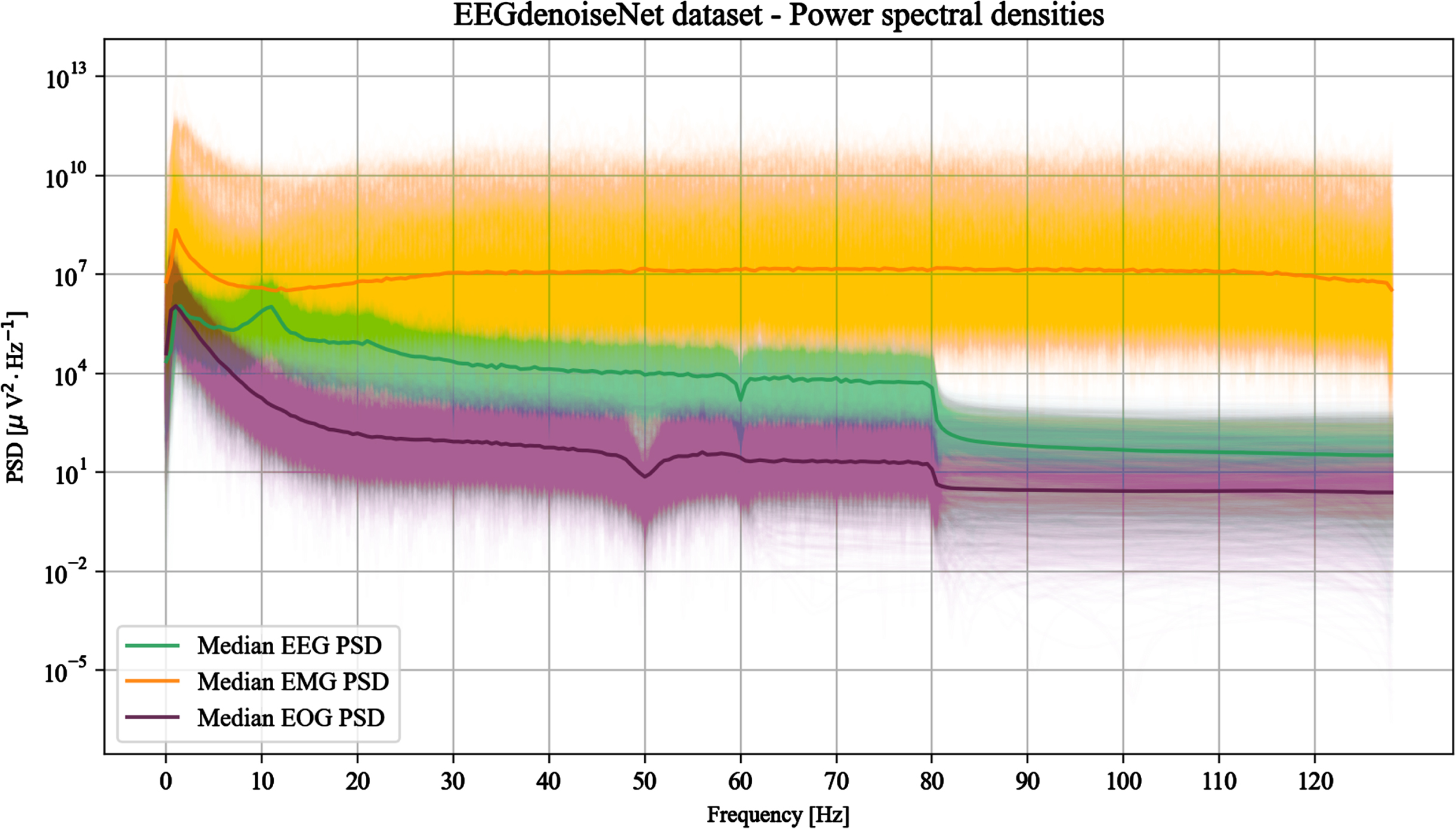
Power spectral densities of 2000 random signals from each type (EEG, EOG and EMG) of the EEGdenoiseNet dataset. The median PSDs are also shown to highlight the overall trend of the different signal types.

Starting from these representations, some observations have been made concerning the filtering performed firstly by the source datasets and secondly by EEGdenoiseNet authors.

Considering the source datasets, the clean EEG signals have been extracted from Cho et al.’s collection [6], whose recordings have been performed in the Republic of Korea and thus with a power line frequency of 60 Hz [1]. While power line noise management is not mentioned by the authors, Fig. 1 reveals that a 60 Hz notch filter has been applied to remove this noise source.

As introduced in Section 3.1, the EOG signals derive instead from three different datasets. The authors of BCI Competition IV dataset 2a and 2b [22, 31] report that the signals were acquired with a 250 Hz sampling rate and filtered with a broadband anti-aliasing bandpass filter between 0.5 and 100 Hz and a 50 Hz notch filter. Instead, Kanoga et al. [15] acquire the signals with a 256 Hz sampling rate and process them with a bandpass filter between 0.5 and60 Hz.

These statements are verified by analysing the trend of the median of the EOG PSDs depicted in Fig. 1. A decrease of the PSD at 50 Hz seems to be related to the notch filter applied to the BCI Competition IV data and a slight decrease at 60 Hz related to Kanoga et al.’s signals. Nevertheless, apparently not all signals present an evident 50 Hz notch and it could be conjectured that these cases belong to the latter dataset.

Finally, for the EMG signals, Rantanen et al. [27] declare the application of 8th order Butterworth filters (zero-phase forward and reverse) to remove the power line noise (50 Hz) and to consider a frequency range between 20 and 500 Hz.

However, discrepancies between the provided statements and the plotted PSDs can be observed (Fig. 1). Neither a noise peak nor a pit due to a notch filter are visible at 50 Hz. Moreover, there is a significant amount of power for low frequencies especially below 10 Hz, suggesting that EEGdenoiseNet uses a raw (unfiltered) version of the EMG signals.

Some discrepancies can be also noticed when analysing the resulting PSDs in respect to the processing declared by the EEGdenoiseNet authors.

According to Zhang et al., the EEG signals are bandpass (1 - 80 Hz) and notch (50 Hz) filtered. While there is clear evidence of the application of the former filter (Fig. 1), the latter does not appear to be applied. Moreover, the declaration of a possible 50 Hz notch filter is contradictory with the clearly visible 60 Hz notch filter applied by Cho et al.

A lack of clarity is also present when analysing the EOG and EMG signals. Bandpass (0.3 - 10 Hz) and notch (50 Hz) filters are declared to be applied to the EOG signals. However, the bandpass filter is not particularly evident.

Similarly, Zhang et al. declare that the EMG data are filtered with a 1 - 120 Hz bandpass and a 50 Hz notch filter. While the bandpass filtering is not particularly evident from Fig. 1, the 50 Hz notch filter seems to be avoided.

In general, the peaks typical of the power line noise are not present in the reported PSDs. However, not all the pits appearing in the PSD plots seem to be associated with the declared filters and there is no particular evidence of the application of the declared bandpass filters.

It should also be noted that the only signals with relatively important frequencies above 80 Hz are the EMG: for EEG and EOG signals frequencies above 80 Hz appear evidently filtered out.

To compare our results with those obtained by the literature benchmark models, we use the EEDdenoiseNet dataset as provided by the authors, without applying any further filter.

3.3 Proposed model

In this work a novel denoising model leveraging data in the frequency domain is proposed.

The idea is that given a prior knowledge about the noise spectral features, an optimal convolutional filter, or a cascade of filters, can be computed to separate the noise from the actual neural signal. Therefore, the proposed model is trained to learn an empirical relationship which connects the spectral characteristics of noise and noisy signal to a non-linear transformation able to denoise that signal. The assumptions under which the model can operate are:

the PSD estimate of the noise is given;

the relation between signal and noise is known.

For the EEGdenoiseNet dataset this relationship is a linear mixture of the clean signal and the artifacts (OAs and MAs considered one at a time) as per Equation (2).

The PSD related to noise λn, the PSD related to noisy signal y, and the noisy signal are all given separately as multiple inputs to the model, which consists of two major components, repeatedly applied: the kernel evaluator and the convolutional filters applier. The kernel evaluator is used to evaluate the best convolutional filters from the frequencies that are characteristic of the noisy signal and noise. The convolutional filters applier then effectively apply the filters estimated by the kernel evaluator to the time domain signal. The overall pipeline of the model is depicted in Fig. 2.

Fig. 2

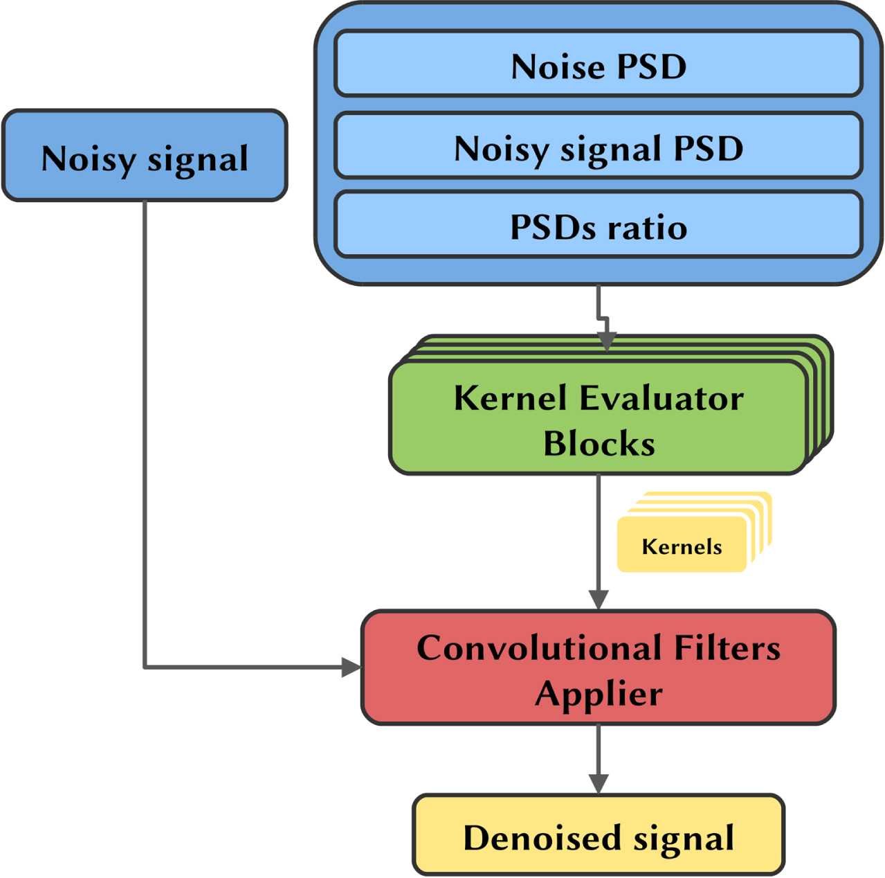
Model pipeline presenting the input form, the model mainly constituted by the kernel evaluator and the convolutional filter applier, and the obtained output.

3.3.1 Model inputs

The model is inputted with two inputs not directly interacting with each other: the PSDs and the time series. The former is the concatenation of the PSD of the pure noise, the PSD of the noisy signal (which is always known) and the ratio between the noisy signal and the pure noise PSDs, which does not add any further information but facilitates model learning since the ratio is an operation not easily reproducible by the following convolutional operations. The PSDs and their ratio are processed by the kernel evaluator blocks only. The latter, i.e., the time series, is the noisy signal in the time domain, which is processed in cascade by the convolutional filters applier block in order to obtain the denoised signal.

3.3.2 Kernel evaluator

For each convolutional step a kernel evaluator block, whose structure is depicted in Fig. 3, evaluates a set of convolutional filters (i.e., the kernels values) to be applied to the time series.

Fig. 3

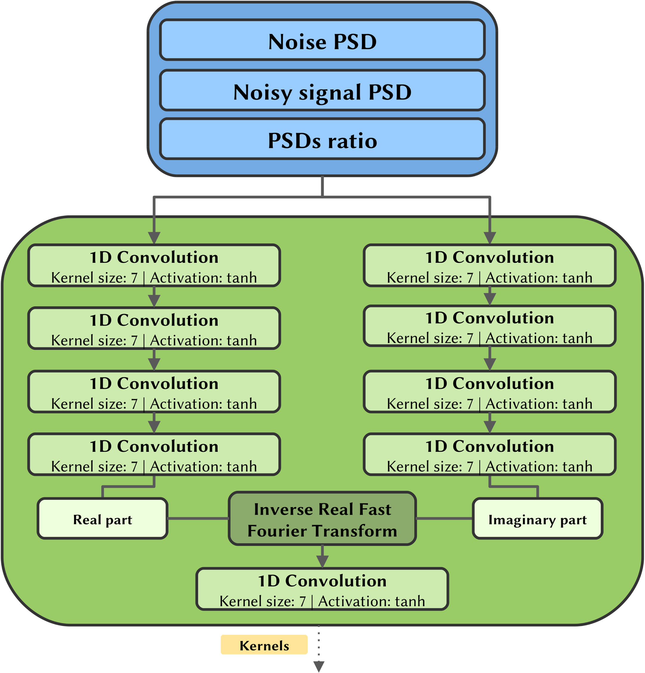
Kernel evaluator block diagram depicting the input form, the kernel evaluator, and its output.

Each block is inputted with the PSDs, which are processed by two symmetric series of 1D convolutional layers with tanh activations. These branches independently estimate the real and imaginary part of the filters that will be subsequently applied to the time series. Remind that in this case the model is working in the frequency domain, dealing with PSDs.

To translate the filters into the time domain, where they will actually operate on the noisy signal, an inverse real fast Fourier transformation (IRFFT) is then applied to the complex 1D arrays obtained by assembling the two branches.

The IRFFT operation adds algorithmic capabilities to the model since the convolutional and activation layers in the pipeline cannot replace it by performing an analogous transformation.

The inverse fast Fourier transform (IFFT) is an algorithm that efficiently computes the inverse discrete Fourier transform (IDFT) of a sequence and is given as follows: $x [n] = \frac{1}{N} \sum_{k = 0}^{N - 1} X [k] e^{i \frac{2 π}{N} kn}$ (3)

The IRFFT is a particular case of IFFT which returns real-valued sequences, as would be desired for the time-domain filters, without sacrificing the useful algorithmic capabilities of the Fouriertransform.

As a final step, the filters outputted by the IRFFT are linearly combined with a 1D convolutional layer with kernel size equal to 1. The last tanh activation forces the filters values in the range [-1 ; 1], avoiding numerical problems coming from too high values and acting as a normalizer on filters.

The length of the filters evaluated by the kernel evaluator block is equal to the length of the input noisy signal itself, thus the filters are able to act on any signal frequency and to extract both local and global features. The kernel evaluator blocks contain all and only the trainable parameters of the model, specifically the kernels of the 1D convolutions applied to the PSDs. Therefore these parameters, which amount to 224192, depend only on the frequency characteristics of the signal and noise. The choice of the number of convolutional layers and the size of the kernels they apply are dictated by having a sufficiently large receptive field that operates on correlated frequencies that are close to each other, without taking into account very distant frequencies.

3.3.3 Convolutional filters applier

The filters evaluated by the kernel evaluator blocks are inputted to the convolutional filter applier, which uses them without further changes. As depicted in Fig. 4, on the first step this part of the model applies 1D convolutions directly to the noisy signal using the filters of the first kernel evaluator block and the resulting features are inputted to an ELU activation function.

Fig. 4

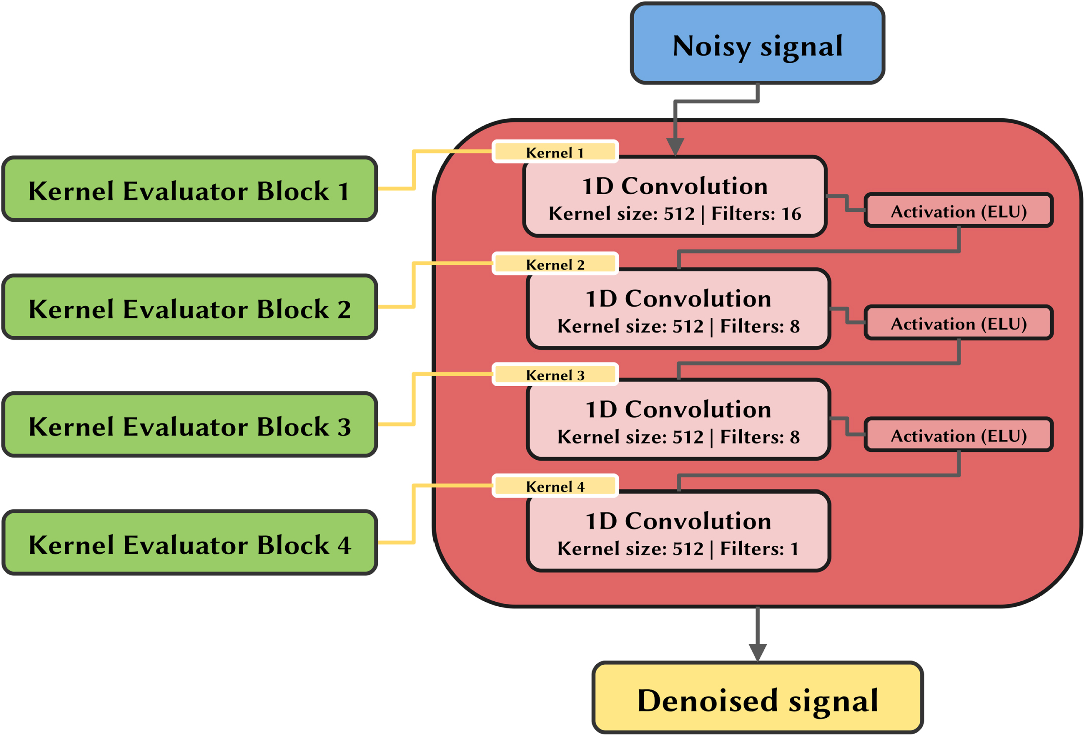
Convolutional filter applier schema using the previously obtained filters as inputs. The output is the denoised signal.

Subsequently, these features are convoluted with the filters evaluated by the second block and once again activated by the ELU function. This operation is repeated in cascade until the last convolution, which returns directly the denoised signal. No activation is applied in this last step and the range of possible values is therefore (- ∞ ; + ∞), which is also the range of the possible clean signals.

The number of convolutions applied in series and the number of filters applied at each convolutional step were sized based on domain knowledge and in a way that limited the total number of parameters trained in the kernel evaluator blocks.

4 Performed experiments

The denoising capabilities of the proposed model are evaluated on the basis of the reconstruction performance of pure EEG signals from the EEGdenoiseNet dataset when contaminated by EOG or EMG artifacts, separately, following the paradigm proposed by the authors of the benchmark model [43] and considered by most of the reported literature works (Section 2). In this section the data preparation method, the metrics used to evaluate the model and the training process are described. Finally, statistical and graphical results of the model are reported.

4.1 Data preparation

The original dataset has been randomly partitioned into two mutually exclusive subsets, i.e., a training set (60%) and a test set (40%). Therefore, the training set consists of 2708 EEG, 3358 EMG and 2040 EOG samples while the test set consists of 1806 EEG, 2240 EMG and 1360 EOG samples.

To synthesize the noisy signals from the pure samples, the linear relation defined in Equation (2) has been used. The λ values are randomly sampled to obtain a uniform distribution of the signal-to-noise ratio (SNR) in the range [-7dB ; 4dB] for the model training and in the range [-7dB ; 2dB] for the model testing. This is a common range for OAs and MAs and the same range has been used by the EEGdenoiseNet authors [43].

During the training phase, the noisy data synthesis is performed runtime in a random way, allowing the model to be trained with constantly new combinations of signal, noise and SNR.

Both noisy signal and pure noise are standardized using the mean and standard deviation of the noisy signal.

4.2 Metrics

In order to quantitatively evaluate the performance of the model in the denoising task, standard metrics used for benchmarking on EEGdenoiseNet data are adopted.

The Root Mean Square Error (RMSE) is used to measure the variance between the output predicted by the model and the ground truth and it is defined by: $RMSE = \sqrt{\frac{\sum_{i = 1}^{N} (x_{i} - {\tilde{y}}_{i})^{2}}{N}}$ (4) where x denotes the EEG signal, $\tilde{y}$ the denoised signal and N the total number of data points of the signal.

To avoid a metric depending on the absolute value of the signals, the Relative Root Mean Square Error (RRMSE) is used, which in the time domain is expressed as follows: ${RRMSE}_{t} = \sqrt{\frac{\sum_{i = 1}^{N} (x_{i} - {\tilde{y}}_{i})^{2}}{\sum_{i = 1}^{N} x_{i}^{2}}}$ (5) while when considering the frequency domain we obtain the following: ${RRMSE}_{f} = \sqrt{\frac{\sum_{i = 1}^{N} (PSD (x)_{i} - PSD (\tilde{y})_{i})^{2}}{\sum_{i = 1}^{N} PSD (x)_{i}^{2}}}$ (6)

The correlation coefficient (CC), also referred to as Pearson correlation coefficient, measures the degree of the statistical relationship between two variables, in this case the ground truth signal and the denoised signal. The CC takes values in the range [-1 ; 1], where ±1 indicates complete linear dependence between the variables, while 0 could mean their independence, and is defined as follows: $CC = \frac{\sum_{i = 1}^{n} (x_{i} - \bar{x}) ({\tilde{y}}_{i} - \bar{y})}{\sqrt{\sum_{i = 1}^{n} (x_{i} - \bar{x})^{2}} \sqrt{\sum_{i = 1}^{n} ({\tilde{y}}_{i} - \bar{y})^{2}}}$ (7)

where $\bar{x}$ and $\bar{y}$ are the means of the ground truth and of the model output, respectively.

4.3 Training process

Standardization helps to speed up the training process since input centering and scaling operations improve the rate at which the neural network converges [18]. Indeed, the learning algorithm is sensitive to the input scale, and if the input data are not standardized, it may take longer for the algorithm to find a good set of parameters, i.e., weights and thresholds of the network, or the learning algorithm may get stuck in a local minima. Moreover, the standardization of the input data makes the model capable of processing EEG signals with wider amplitude ranges. Nevertheless, only the mean and standard deviation of the noisy signal are always known. Therefore, the noisy signal y, the pure EEG signal x and the pure noise n are processed in a similar manner according to: $\hat{x} = \frac{x - \bar{y}}{σ_{y}}, \hat{y} = \frac{y - \bar{y}}{σ_{y}}, \hat{n} = \frac{n - \bar{y}}{σ_{y}}$ (8)

These signals, as well as the PSDs evaluated by them, are the actual inputs of the model.

The loss function minimized in the training phase is a combination of three different terms, differently weighted: $L = a L_{{RRMSE}_{t}} + b L_{{RRMSE}_{f}} + c L_{\log - \cosh}$ (9)

where L_{RRMSE
_t} is the temporal RRMSE defined in Equation (5), L_{RRMSE
_f} is the spectral RRMSE defined in Equation (6), and L_log-cosh the log-cosh error of the ground truth and predicted signals in the time domain, which is defined by the equation: $L_{\log - \cosh} (x, \tilde{y}) = \sum_{i = 1}^{N} log (cosh ({\tilde{y}}_{i} - x_{i}))$ (10)

This function provides a smooth approximation to the mean absolute error for values near 0. The a, b,and c coefficients are empirically chosen for the training and are equal to 0.25, 0.25, and 0.5, respectively.

The optimization method used to find the best weights of the kernel evaluator blocks is AdaMax [16].

The code was developed in Python 3.8.10 and the proposed model was designed using the TensorFlow library, version 2.8. The experiments were run on an Nvidia Quadro RTX 4000 for a total training time of 61 hours.

5 Results

A single model has been trained on both EMG and EOG artifacts at the same time in order to have a solution capable of handling both cases. In fact, the noisy signals are affected by either OAs or MAs. Therefore, both EMG only and EOG only affected signals are inputted to the model, as introduced at the beginning of Section 4.

Figure 5 shows the trend of loss as the epochs change for the training and test sets. For both datasets the loss values monotonically decrease and no significant overfit is present. This indicates that the model design and the used runtime data synthesis approach are effective in avoiding this issue.

Fig. 5

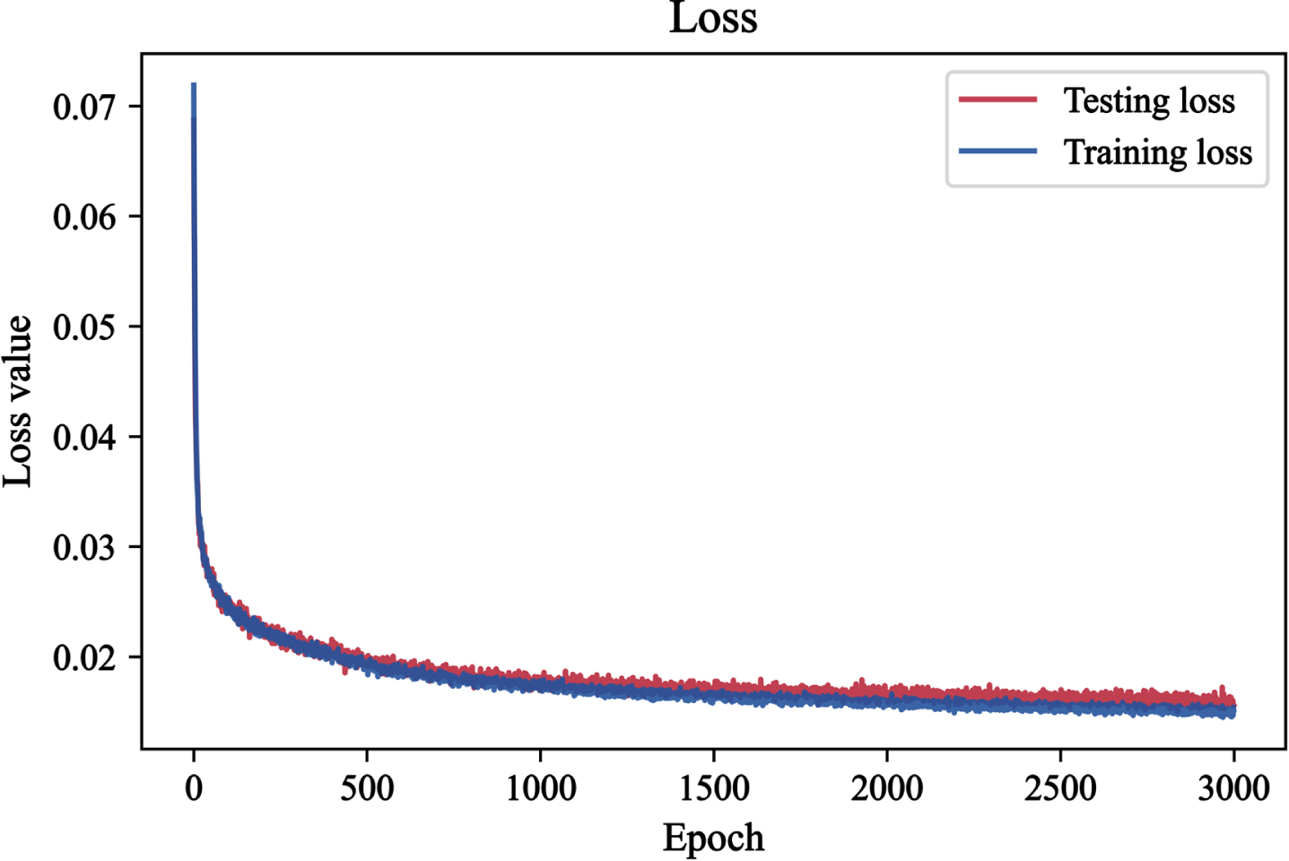
Loss of the training set and test set as training epochs increase.

Using the last epoch weights, the denoising capabilities of the model on EOG and EMG artifacts are qualitatively demonstrated. Figures 6 and 7 show examples of the model outcome when facing signals corrupted by OAs and MAs (–7 dB SNR), respectively. We can observe that both the high frequencies related to MAs and low frequencies related to OAs are filtered by the model. The majority of the morphological structures related to the clean EEG signals are preserved, while the typical V-shaped OAs and high amplitude MA signals are attenuatedor removed.

Fig. 6

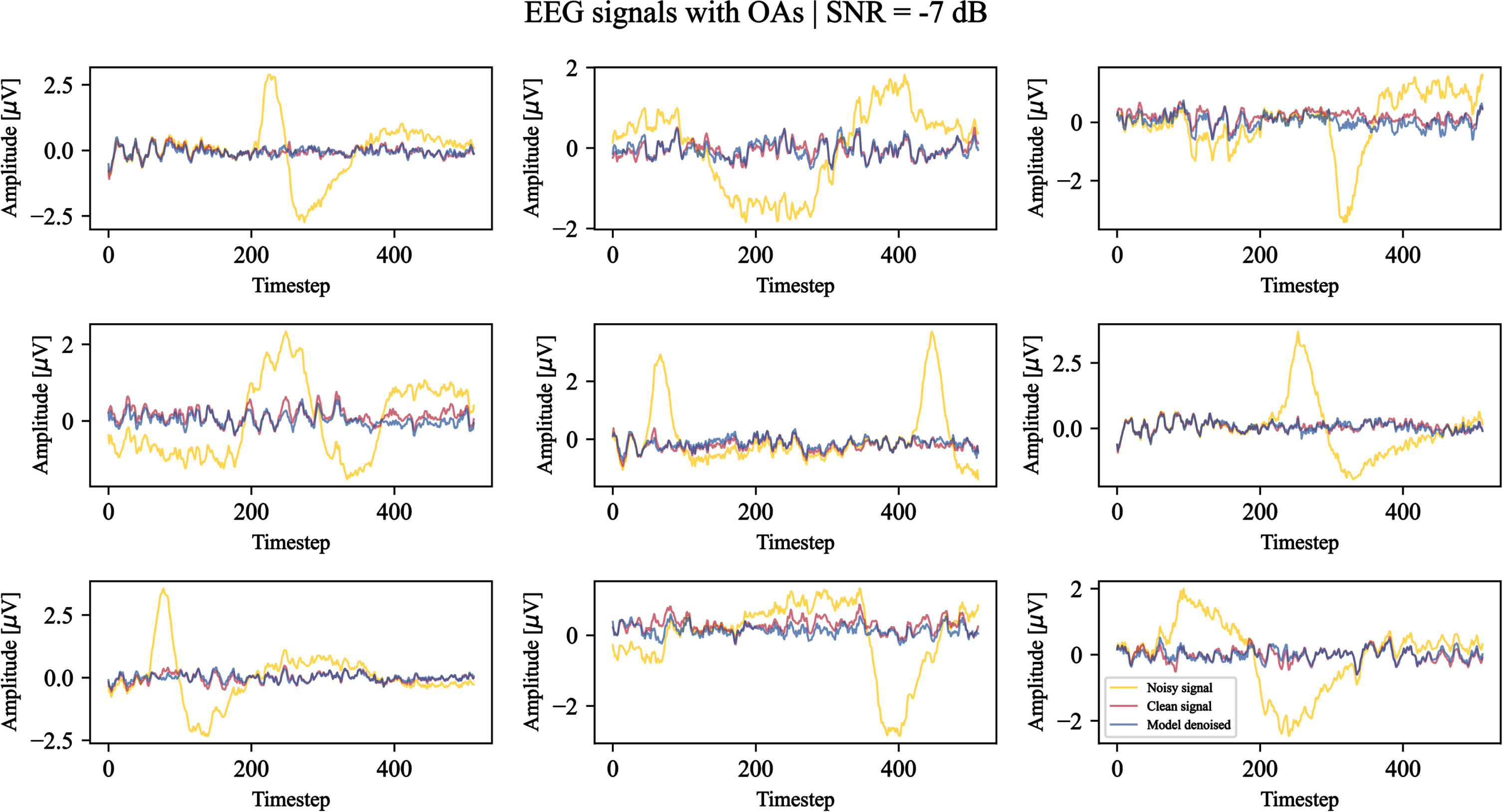
Nine test examples of noisy EEG signals corrupted by ocular artifacts with a signal-to-noise ratio equal to –7 dB denoised by the model. For each example, the original noisy signal is shown in yellow, the clean ground truth signal is shown in red, and the model-denoised signal is shown in blue. The timestep denotes the signal sample.

Fig. 7

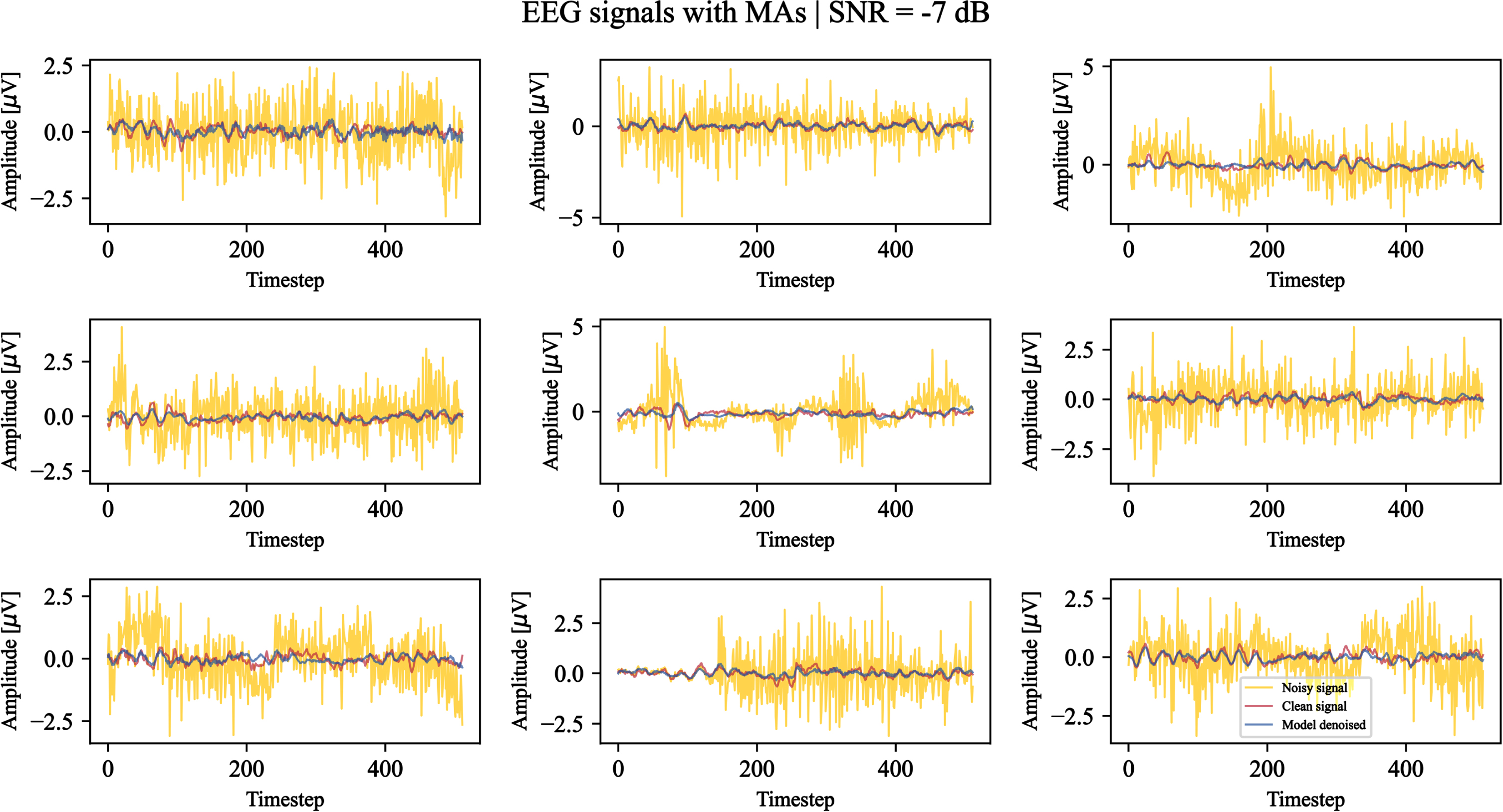
Nine test examples of noisy EEG signals corrupted by muscular artifacts with a signal-to-noise ratio equal to –7 dB denoised by the model. For each example, the original noisy signal is shown in yellow, the clean ground truth signal is shown in red, and the model-denoised signal is shown in blue. The timestep denotes the signal sample.

In general, several amplitude ranges are properly managed by the model as well as different SNRs.

The quantitative results of the proposed model and of the literature benchmark models for MAs and OAs are reported in Tables 1 and 2, respectively.

Table 1

Metrics of the proposed denoising model and benchmark models averaged on all SNRs ([-7dB ; 2dB]) with noisy signals affected by MAs

Model	RRMSE _t	RRMSE _f	CC
FCNN [42]	0.585	0.580	0.796
Simple CNN [42]	0.646	0.649	0.783
Complex CNN [42]	0.650	0.633	0.780
RNN [42]	0.570	0.530	0.812
Novel CNN [42]	0.448	0.442	0.863
DeepSeparator [41]	0.712	0.717	0.734
EEGDnet [26]	0.677	0.626	0.732
Proposed model	0.573	0.496	0.805

Table 2

Metrics of the proposed denoising model and benchmark models averaged on all SNRs ([-7dB ; 2dB]) with noisy signals affected by OAs

Model	RRMSE _t	RRMSE _f	CC
DeepSeparator [41]	0.705	0.747	0.769
EEGDnet [26]	0.497	0.491	0.868
Proposed model	0.405	0.490	0.917

The results reported from the literature have all been consistently evaluated on a dataset of noisy signals having a uniformly distributed SNR in the range [-7dB ; 2dB], which is the one originally used by the authors of EEGdenoiseNet and, subsequently, the one typically adopted by users of this dataset. The results reported by other authors, such as Dong et al., who made different choices in the application of the artifacts resulting in different SNR distributions in the test data, are therefore not comparable with those obtained in this work and are not reported.

Regarding EEG affected by MAs, the reported values are in line with the benchmark models results. The proposed model demonstrated robust performance, achieving the third best results in the temporal domain metrics, RRMSE_t and CC, and the second best result in the spectral metric RRMSE_f. The latter metric provides insights into the method ability to effectively preserve the spectral information of the clean EEG signal. We remind that the model design was intended for this particular preservation, considering the spectral characteristics of noise and noisy signals. Thus achieving better or coherent RRMSE_f values in respect to the literature represented one of the main aims of this work.

Concerning OAs, our method achieves the best performance on all three metrics among the reported benchmark models. Furthermore, the similarity of the proposed model results in RRMSE_f values on both muscular and ocular artifacts highlights the method stability and its ability to perform indiscriminately well on both high and low frequencies.

In contrast to the current state-of-the-art, the proposed model is able to achieve these results using not only a single architecture but also a single set of trained parameters, valid on both MAs and OAs. This allows the two main sources of noise in EEG signals to be handled with a single solution.

6 Discussion

The proposed denoising model relies on the PSD estimation of noise-affected EEG signals and of the sources from which the artifacts affecting the neural data are generated, namely EOG and EMG signals.

Considering the presented results (Section 5), the model is able to discriminate the spectral information of neural, OA, and MA data by a large amount, maintaining the EEG signal characteristics, while suppressing the noisy components.

However, while the need to have as input an estimate of the PSD of the noise afflicting the signal makes the method more adaptable to new noise conditions with known characteristics, it also makes it sensitive to precise a priori knowledge of the frequency characteristics of this noise that cannot be easily estimated.

In the future, methods trained on the reference dataset to best estimate the PSD of the noise of each signal as a substitute for the exact PSD provided in the current work will be developed.

Moreover, besides understanding the reason why some discrepancies are present when analysing the spectral component of EEGdenoiseNet in respect to the described processing of its source datasets (as presented in Section 3.2) and assessing the reliability of the clean EEG ground truth obtained through the application of ICLabel, other datasets will be used to ensure the generalizability of the proposed methodology. In fact, it could be possible that the models trained on synthetic datasets, such as EEGdenoiseNet, are not portable to diverse real-world datasets. Major concerns would then be how much the unique characteristics of the training dataset can impact the performance of the algorithm when applied to real data, and how much the trained features can be leveraged to enhance the outcomes in related tasks involving EEG signals. In the majority of cases, the literature models developed on the EEGdenoiseNet dataset are not applied to additional datasets for further validation purposes. In contrast, Yu et al. [41] applied their denoising algorithm to real datasets and achieved encouraging qualitative results in the tasks for which this processing was used. However, they were unable to provide quantitative evaluations due to the absence of actual ground truth data. With the aim of quantitatively evaluating the ability of the algorithm developed in this work to improve the interpretability of neural data, we intend to investigate how this model can best be applied to other datasets in the future. In this direction, the proposed algorithm could be used as a preprocessing step in classification problems of different types of imagined movements or cognitive tasks.

As an alternative to EEGdenoiseNet or other existing datasets, very recent studies [8, 23] have introduced their own datasets to validate DL-based denoising models.

As for EEGdenoiseNet, Chuang et al. [8] consider the use of the ICLabel toolbox to extract a clean target for their DL model from an in-house resting-state experiment. The authors mark independent components as neural signals when the probability of these components being brain activity is grater than 80%. Non-brain activities are instead marked as muscular, ocular, cardiac, line and channel noise, or other. The mixing of clean and noise components seems to consider a single artifact at a time. Notably, besides using the in-house dataset, the authors validate their IC-U-Net model by considering synthetic data, a simulated driving experiment and real walking data [7], and the BCI Challenge@NER 2015 collection (https://kaggle.com/competitions/inria-bci-challenge). For completeness notice that the proposed IC-U-Net combines independent component analysis and U-Net to design a deep denoising autoencoder that tries to approximate the clean target by minimising an ensemble of loss functions. In fact, the authors wanted to linearly combine four terms covering signal amplitude, velocity, acceleration, and frequency, thus considering a broader range of EEG signal characteristics.

Instead, Narmada and Shukla [23] consider two levels of noise removal. Firstly, the authors apply empirical mode decomposition [12] and adaptive artifact wavelet denoising based on the discrete wavelet transform [9], and then an Improved-CycleGAN with opposition searched-elephant herding optimization. The authors consider two EEG datasets and combine the neural data with three different artifacts, i.e., muscular, ocular, and cardiac artifacts. Notice that the combination is provided by considering one artifact type at a time, and that all the signals come from different data sources.

Surely, the ability of DL-based methodologies to remove singularly different types of artifacts is fundamental. However, future works and further developments of the model proposed in this study should be able to remove multiple artifacts at the same time as in real case scenarios. Considering that the clean/noisy EEG couples could influence DL-model performance [8], it could be also argued the necessity of providing reliable benchmarking datasets presenting the recordings of EEG signals as well as noise source reference data acquired using EMG, EOG, electrocardiogram and accelerometer at the same time.

However, obtaining a great amount of ground truth data is difficult, although it is necessary to ensure the devised strategy ability of modeling different signal mixtures [11].

Besides the difficulties deriving from requiring volunteers to sit for a long time to perform experiments, the possibility of noise content overly exceeding the brain-related information, could pre-empt the application of any denoising technique. In fact, they could result ineffective and provide an outcome incoherent with a real neural response. Therefore, while the manual rejection of EEG signal portions is based on the operator expertise and relatively time consuming [21], the visual inspection of the dataset may be necessary to understand the overall dataset quality and possibly detect excessively noisy signal segments before performing further processing steps.

Still on the influence of data on the quality of the trained deep learning model, it could be questioned whether the use of a dataset with a discrete set of possible SNRs rather than a continuous range of values might result in a different ability of the models to generalise to artifacts of varying intensity. Such an evaluation might allow the addition of further benchmark models, such as the one proposed by Hossain et al. [11] that use discrete rather than continuous values of SNRs as in this work, for a more complete model validation.

A better denoising of EEG signals could be also achieved by considering different activation functions and artifact amount estimation methodologies [34], as well as the modeling of specific loss functions [10].

Moreover, Dong et al. highlight that the majority of the models treats all the channels in the same way by processing them one at a time [10]. However, this may result in a loss of spatial information, which could be exploited to better understand inter-channel relationships and their possible interference. Therefore, this information could be considered for further developments of the proposed model.

In future works we will also provide a rigorous assessment on the possible improvement of classification performances due to the decrease of noisy components after the application of a DL-based denoising technique. Furthermore, DL-models relying on filter banks as well as more standard filter bank common spatial pattern (FBCSP) [2] based algorithms will be considered for additional comparisons with the literature, having that they have been employed in different EEG applications. For example, Jia et al. [13] have proposed the use of a filter bank task-related component analysis composed of spatial filtering for noise removal, similarity measuring for feature extraction, and filter bank selection. Parallel filter bank CNNs have been also developed for motor imagery classification to consider both temporal and spatial features [38]. Finally, FBCSP strategies have been exploited to find suitable narrow-bands for motor imagery tasks before applying a deep CNN [39].

7 Conclusions

The significant issue of muscle and ocular artifact removal in EEG data has been tackled in this research. We introduced a unique solution capable of dealing with both artifact types using a single model. Our proposed method leverages dynamically assessed convolutional filters, which are determined based on the frequency features of the noise and the noisy signal. With this knowledge, our model has proven its effectiveness in both qualitatively and quantitatively cleaning EEG signals from muscle and ocular artifacts. This achievement either matches or exceeds the performance of existing state-of-the-art models, which typically require specific training on either ocular or muscle artifacts. Thus, this study marks a substantial step forward in EEG data processing by offering a versatile spectral-based strategy for artifacts elimination and provides a baseline for subsequent work addressing the problem of estimating noise frequencies, whether with experimental solutions, algorithmic solutions, or a combination of the two.

Conflict of interest

The authors declare no competing interests.

Footnotes

Acknowledgements

This work was partially supported by the MUR under the grant “Dipartimenti di Eccellenza 2023-2027” of the Department of Informatics, Systems and Communication of the University of Milano-Bicocca, Italy.

References

Iec world plugs. https://www.iec.ch/world-plugs. Accessed: 2024-01-28.

Ang

K.K.

, Chin

Z.Y.

, Zhang

, Guan

, Filter bank common spatial pattern (fbcsp) in braincomputer interface. In 2008 IEEE International Joint Conference on Neural Networks (IEEE world congress on computational intelligence), (2008), pp. 2390–2397. IEEE.

Asadi-Aghbolaghi

, Azad

, Fathy

, Escalera

, Multi-level context gating of embedded collective knowledge for medical image segmentation, arXivpreprint arXiv:2003.05056, 2020.

Brophy

, Redmond

, Fleury

, De Vos

, Boylan

, Ward

, Denoising EEG Signals for Real-World BCI Applications Using GANs, Frontiers in Neuroergonomics2 (2022), 44.

Chen

, Xu

, Liu

, Lee

, Chen

, Zhang

, McKeown

M.J.

, Wang

Z.J.

, Removal of muscle artifacts from the EEG: A review and recommendations, IEEE Sensors Journal19(14) (2019), 5353–5368.

Cho

, Ahn

, Kwon

, Jun

S.C.

, EEG datasets for motor imagery brain–computer interface, GigaScience6(7) (2017), gix034.

Chuang

C.-H.

, Ko

L.-W.

, Jung

T.-P.

, Lin

C.-T.

, Kinesthesia in a sustained-attention driving task, Neuroimage91 (2014), 187–202.

Chuang

C.-H.

, Chang

K.-Y.

, Huang

C.-S.

, Jung

T.-P.

, IC-U-Net: a U-Net-based denoising autoencoder using mixtures of independent components for automatic EEG artifact removal, NeuroImage263 (2022), 119586.

Daubechies

, Ten lectures on wavelets, SIAM, 1992.

10.

Dong

, Tang

, Li

, Wang

, Jiang

, Tian

, Zheng

, Li

, Zhao

, Li

, et al., An Approach for EEG Denoising Based on Wasserstein Generative Adversarial Network, IEEE Transactions on Neural Systems and Rehabilitation Engineering, 2023.

11.

Hossain

Md S.

, Mahmud

, Khandakar

, Al-Emadi

, Chowdhury

F.A.

, Mahbub

Z.B.

, Ibne Reaz

M.B.

, Chowdhury

M.E.H.

, MultiResUNet3+: A Full-Scale Connected Multi-Residual UNet Model to Denoise Electrooculogram and Electromyogram Artifacts from Corrupted Electroencephalogram Signals, Bioengineering10(5) (2023), 579.

12.

Huang

N.E.

, Shen

, Long

S.R.

, Wu

M.C.

, Shih

H.H.

, Zheng

, Yen

N.-C.

, Tung

C.C.

, Liu

H.H.

, The empirical mode decomposition and the hilbert spectrum for nonlinear and non-stationary time series analysis, Proceedings of the Royal Society of London. Series A: mathematical, physical and engineering sciences454(1971) (1998), 903–995.

13.

Jia

, Feng

, Caiafa

C.F.

, Duan

, Zhang

, Sun

, Sole-Casals

, Multi-class classification of upper limb movements with filter bank task-related component analysis, IEEE Journal of Biomedical and Health Informatics, 2023.

14.

Jiang

, Bian

G.-B.

, Tian

, Removal of artifacts from EEG signals: a review, Sensors19(5) (2019), 987.

15.

Kanoga

, Nakanishi

, Mitsukura

, Assessing the effects of voluntary and involuntary eyeblinks in independent components of electroencephalogram, Neurocomputing193 (2016), 20–32.

16.

Kingma

D.P.

, Ba

, Adam: A method for stochastic optimization, arXiv preprint arXiv:1412.6980, 2014.

17.

Koelstra

, Muhl

, Soleymani

, Lee

J.-S.

, Yazdani

, Ebrahimi

, Pun

, Nijholt

, Patras

, Deap: A database for emotion analysis; using physiological signals, IEEE Transactions on Affective Computing3(1) (2011), 18–31.

18.

LeCun

, Bottou

, Orr

G.B.

, Muller

K.-R.

, Efficient backprop. In Neural networks: Tricks of the trade, (2002), pp. 9–50. Springer.

19.

Mannan

M.M.N.

, Kamran

M.A.

, Jeong

M.Y.

, Identification and removal of physiological artifacts from electroencephalogram signals: A review, Ieee Access6 (2018), 30630–30652.

20.

Minguillon

, Lopez-Gordo

M.A.

, Pelayo

, Trends in EEG-BCI for daily-life: Requirements for artifact removal, Biomedical Signal Processing and Control31 (2017), 407–418.

21.

Mumtaz

, Rasheed

, Irfan

, Review of challenges associated with the EEG artifact removal methods, Biomedical Signal Processing and Control68 (2021), 102741.

22.

Naeem

, Brunner

, Leeb

, Graimann

, Pfurtscheller

, Seperability of four-class motor imagery data using independent components analysis, Journal of Neural Engineering3(3) (2006), 208.

23.

Narmada

, Shukla

M.K.

, A novel adaptive artifacts wavelet Denoising for EEG artifacts removal using deep learning with Meta-heuristic approach, Multimedia Tools and Applications, (2023), pp. 1–39.

24.

Ozdemir

M.A.

, Kizilisik

, Guren

, Removal of Ocular Artifacts in EEG Using Deep Learning. In 2022 Medical Technologies Congress (TIPTEKNO), (2022), pp. 1–6. IEEE.

25.

Pion-Tonachini

, Kreutz-Delgado

, Makeig

, ICLabel: An automated electroencephalographic independent component classifier, dataset, and website, NeuroImage198 (2019), 181–197.

26.

, Yi

, Chen

, Ma

, Zhao

, Ren

, EEGDnet: Fusing non-local and local selfsimilarity for EEG signal denoising with transformer, Computers in Biology and Medicine151 (2022), 106248.

27.

Rantanen

, Ilves

, Vehkaoja

, Kontunen

, Lylykangas

, Makela

, Rautiainen

, Surakka

, Lekkala

, A survey on the feasibility of surface EMG in facial pacing. In 2016 38th Annual International Conference of the IEEE Engineering in Medicine and Biology Society (EMBC), (2016), pp. 1688–1691. IEEE.

28.

Rashmi

C.R.

, Shantala

C.P.

, EEG artifacts detection and removal techniques for brain computer interface applications: a systematic review, International Journal of Advanced Technology and Engineering Exploration9(88) (2022), 354.

29.

Ronneberger

, Fischer

, Brox

, Unet: Convolutional networks for biomedical image segmentation. In Medical Image Computing and Computer-Assisted Intervention–MICCAI 2015:18th International Conference, Munich, Germany, October 5-9, 2015, Proceedings, Part III 18, (2015), pp. 234–241. Springer.

30.

Saibene

, Caglioni

, Corchs

, Gasparini

, EEG-Based BCIs on Motor Imagery Paradigm UsingWearable Technologies: A Systematic Review, Sensors23(5) (2023), 2798.

31.

Schlogl

, Keinrath

, Zimmermann

, Scherer

, Leeb

, Pfurtscheller

, A fully automated correction method of eog artifacts in eeg recordings, Clinical Neurophysiology118(1) (2007), 98–104.

32.

Tangermann

, Muller

K.-R.

, Aertsen

, Birbaumer

, Braun

, Brunner

, Leeb

, Mehring

, Miller

K.J.

, Mueller-Putz

, et al., Review of the BCI competition IV, Frontiers in Neuroscience, (2012), pp. 55.

33.

Uriguen

J.A.

, Garcia-Zapirain

, EEG artifact removal—state-of-the-art and guidelines, Journal of Neural Engineering12(3) (2015), 031001.

34.

Vialatte

F.-B.

, Sole-Casals

, Cichocki

, EEG windowed statistical wavelet scoring for evaluation and discrimination of muscular artifacts, Physiological Measurement29(12) (2008), 1435.

35.

Wallstrom

G.L.

, Kass

R.E.

, Miller

, Cohn

J.F.

, Fox

N.A.

, Automatic correction of ocular artifacts in the EEG: a comparison of regression-based and component-based methods, International Journal of Psychophysiology53(2) (2004), 105–119.

36.

Wang

, Luo

, Shen

, An improved Generative Adversarial Network for Denoising EEG signals of brain-computer interface systems. In 2022 China Automation Congress (CAC), (2022), pp. 6498–6502. IEEE.

37.

Wang

, Li

, Wang

, A novel end-to-end network based on a bidirectional GRU and a selfattention mechanism for denoising of electroencephalography signals, Neuroscience505 (2022), 10–20.

38.

, Niu

, Li

, Fu

, Shi

, Dong

, A parallel multiscale filter bank convolutional neural networks for motor imagery eeg classification, Frontiers in Neuroscience13 (2019), 1275.

39.

, Zhu

, Kong

, Peng

, Hu

, Cao

, A novel classification method for eeg-based motor imagery with narrow band spatial filters and deep convolutional neural network, Cognitive Neurodynamics (2022), pp. 1–11.

40.

Yin

, Liu

, Li

, Qian

, Chen

, Frequency Information Enhanced Deep EEG Denoising Network for Ocular Artifact Removal, IEEE Sensors Journal22(22) (2022), 21855–21865.

41.

, Li

, Lou

, Wei

, Liu

, Embedding decomposition for artifacts removal in EEGsignals, Journal of Neural Engineering19(2) (2022), 026052.

42.

Zhang

, Wei

, Zhao

, Liu

, Wu

, A novel convolutional neural network model to remove muscle artifacts from EEG. In ICASSP 2021-2021 IEEE International Conference on Acoustics, Speech and Signal Processing (ICASSP), (2021), pp. 1265–1269. IEEE.

43.

Zhang

, Zhao

, Wei

, Mantini

, Li

, Liu

, EEGdenoiseNet: a benchmark dataset for deep learning solutions of EEG denoising, Journal of Neural Engineering18(5) (2021), 056057.

44.

Zhang

, Yin

, Chen

, Nichele

, Emotion recognition using multi-modal data and machine learning techniques: A tutorial and review, Information Fusion59 (2020), 103–126.

45.

Zhang

, Yu

, Rong

, Iwata

, A Novel Multimodule Neural Network for EEG Denoising, IEEE Access10 (2022), 49528–49541.

DL-based multi-artifact EEG denoising exploiting spectral information

Abstract

Keywords

1 Introduction

2 Related works

3.1 Dataset

3.3.2 Kernel evaluator

4.1 Data preparation

4.2 Metrics

7 Conclusions

Conflict of interest

Footnotes

Acknowledgements

References