In this article, we construct a Jacobi spectral collocation scheme to approximate the Caputo fractional derivative based on Jacobi–Gauss quadrature. The convergence analysis is provided in anisotropic Jacobi-weighted Sobolev spaces. Furthermore, the convergence rate is presented for solving Caputo fractional derivative with noisy data by invoking the mollification regularization method. Lastly, numerical examples illustrate the effectiveness and stability of the proposed method.
Fractional calculus and derivative is a branch of mathematics that deals with the generalization of integration and differentiation to non-integer orders. It has been verified that substantial physical systems in science and engineering such as fractals, anomalous diffusion, viscoelastic materials, porous or fractured media and viscous fluid flows, can be modeled more effectively by invoking fractional-order rather than integer-order derivatives [2,14,22] due to the cumulative memory effect of wall-friction [5,12,21].
There are extensive amount of work to calculate the fractional derivative numerically over the recent decades years. Lin and Xu [13] developed a hybrid scheme for time-fractional diffusion problem, discretizing the time-fractional derivative by using Finite Difference Method and treating the integer-order spatial derivative by a Legendre spectral method, and rigorously established that the global error is dominated by the low-order temporal accuracy. Zayernouri and Karniadakis [23–25] first introduced fractional Lagrange interpolants to construct the exponentially accurate fractional spectral collocation method to solving fractional Sturm–Liouville eigenproblems and linear/nonlinear fractional partial differential equations with field-variable order. And their numerical results well confirmed the exponential convergence of the fractional collocation methods. Esmaeili and Milovanović[7] derived a numerical scheme to calculate the usual fractional derivative by applying nonstandard Gauss–Jacobi–Lobatto quadratures, and implemented the scheme by using a Mathematica package of Orthogonal Polynomials but without any convergence analysis. Chen et al. [3] constructed Petrov–Galerkin methods for a class of fractional differential equations by employing generalized Jacobi functions. Their numerical results and theoretical analysis demonstrated exponential convergence for the exact solution to be non-smooth except specific singularity. Chen et al. [4] proposed a fast algorithm to solve a subdiffusion problem, which contains Caputo time-fractional derivative with order . They developed a spectral-Galerkin method in time with Log orthogonal functions by applying a log mapping to the Laguerre functions and the Galerkin finite element method in space. They obtained an error estimate with spectral accuracy in time for weakly singular solutions and numerically confirmed the theoretical results. Mao and Karniadakis [15] studied a one-dimensional diffusion equation with general two-sided fractional derivative. They derived a Sturm–Liouville eigenproblem with the two-sided Jacobi polyfractonomials as eigenfunctions by employing a Petrov–Galerkin projection method. They obtained an exponential convergence and numerical examples verified the theoretical results. Dehghan and Mingarelli [6] presented a general solution of three distinct fractional Sturm–Liouville eigenvalue problems, which consist of various compositions of Riemann–Liouville and Caputo fractional derivatives. Nie et al. [18] numerically approximated a fractional sub-diffusion equation with Laplace operator, by employing a modified central finite difference scheme in spatial direction and two kinds of averaged schemes(averaged and averaged second order backward difference scheme) to discretize the Riemann–Liouville fractional derivative in temporal direction. And obtain a better spatial convergence instead of , and an temporal convergence for all fractional order . Jin and Zhou [11] considered an inverse problem of reconstructing a spatial-temporal diffusion coefficient in the sub-diffusion model from the distributed observation. They calculated numerically the direct problem by using the backward Euler convolution quadrature in time to approximate the Caputo fractional derivative of order , and the Galerkin Finite Element Method in space. They provided a complete error analysis of the fully discrete algorithm and established two conditional stability results theoretically by invoking a novel test function, and numerical experiments in agreement with the theoretical analysis. Motivated by the link between singular kernel of Caputo derivative and weight functions of Jacobi polynomials, we desire to study a fast and high accuracy numerical scheme for fractional derivative with order by using Jacobi spectral collocation method, and provide the convergence analysis for calculating numerical fractional derivative from data with noise by mollification regularization method.
The rest of this paper is organized as follows. In Section 2, we introduce some results about Gaussian quadrature and Jacobi orthogonal polynomials. In Section 3, we construct the Jacobi collocation method for Caputo fractional derivatives using the Jacobi weights and polynomials. The convergence analysis for the numerical algorithm are presented in Section 4. In Section 5, the convergence rate is described by virtue of the mollification regularization method when data function f contains noise. Several numerical tests are performed to demonstrate the accuracy and efficiency of the proposed method in Section 6. The paper is concluded in Section 7.
Preliminaries
For the purpose of readability, we state some properties and conclusions about the Gaussian quadrature and Jacobi polynomials in this section. We refer the reader to, for example, [1,8,10,20] and [9] for more details.
The mechanism of a Gauss-type quadrature is to seek the best numerical approximation of an integral by selecting optimal nodes at which the integrand is evaluated. It belongs to the family of the numerical quadratures:
where is the weight function, are the quadrature nodes and weights, and if , the truncated error satisfies
The Jacobi polynomials with parameters α and β, denoted by , are orthogonal with respect to the Jacobi weight function over the interval , namely,
where the weight function belongs to if and only if .
In fact, the Jacobi polynomials are the eigenfunctions of a singular Sturm–Liouville operator defined by
More precisely, the following properties of Jacobi polynomials are hold.
Let Jacobi–Gauss nodesbeing the zeros of the Jacobi polynomialsand the corresponding weights given bywherethen the following Jacobi–Gauss quadrature formulais exact (namely,) for anywith Jacobi–Gauss quadrature pairs.
([20, Differentiation Matrix in the Physical Space]).
Letbe a set of Jacobi–Gauss-type points, andbe the associated Lagrange basis polynomials. Assume thatis an approximation of the unknown solution thenDenotethen the following properties holdswhereandis called the first-order differentiation matrix in the physical space.
Notice that all the nodes of Gauss formula lie in the interior of the interval . Below, in order to impose potential boundary conditions in partial differential equations, we consider the Gauss–Lobatto quadrature which include both endpoints as nodes, and the similar conclusions for Gauss-Radau quadrature can be derived straightforwardly through the same idea.
Jacobi spectral method for Caputo fractional derivatives
Without loss of generality, we just focus on computations of the Caputo fractional derivative. The left-side Caputo fractional derivative with order , is defined by [19]
In view of the weakly singular kernel, we consider the spectral approximation based on the Jacobi–Gauss–Lobatto points to construct the Jacobi-collocation method.
Let be a set of the Jacobi–Gauss–Lobatto points and weights with , , and the linear transform
maps points into , then we have
and the corresponding Jacobi-collocation method for (22) is:
In the light of the first-order differentiation matrix
the scheme (23) becomes
or the matrix form
where
and is the first-order differentiation matrix defined by (19).
The numerical scheme (26) for left-side Caputo fractional derivative can be easily extend to calculating left-side Riemann–Liouville fractional derivative by taking advantage of the well-known relation between Caputo and Riemann–Liouville derivative, :
where is left-side Riemann–Liouville fractional derivative.
Next, we will analyze the error of scheme (25), which approximate the Caputo fractional derivative (20) in anisotropic Jacobi-weighted Sobolev spaces.
Convergence analysis
For simplicity, we assume that the points and are the same (Jacobi–Gauss–Lobatto), although they can be chosen differently in type and in number. For clarity of presentation, we introduce the non-uniformly Jacobi-weighted Sobolev space:
equipped with the inner product, norm and semi-norm
Let and be the weighted continuous and discrete inner product, respectively, and be the corresponding interpolation operator. Then we introduce some lemmas as follows.
For any non-negative integer r and, there exists a linear transformsuch thatwhereis a positive constant,is the space of functions whose r-th derivatives are Hölder continuous with exponent κ, endowed with the usual norm
Letbe the Lagrange basis polynomials associated with the Jacobi–Gauss–Lobatto interpolations with the parameter pair. Then, for, we have
Next, we reveal the error estimate between the exact value and Jacobi collocation approximation for Caputo fractional derivative as Theorem 1.
Assumewith,andfor certain integer. Then we have the estimate:where c is a positive constant independent of N, m and f.
We rewrite (22) and (25) respectively as follows
Denote , then we have
where
equivalently, we write (37) as
Consequently,
where
Now, we estimate the four terms on the right hand side of (40). Firstly, by using [20, Theorem 3.43] and Cauchy–Schwarz inequality, we have
To estimate , let be the Legendre-Gauss–Lobatto polynomial interpolation operator. The Sobolev inequality gives
From Lemmas 5-6 and [20, Lemma 5.2], we obtain
By Lemma 6, we yield
The definition shows that
Therefore, we have
where the above is a positive constant independent of N, m and f.
Finally, a combination of (40), (41), (42), (43) and (46) leads to the estimate (34). □
Mollification regularization and its convergence analysis
Thereafter, we consider the mollification regularization of the numerical scheme (26) when function f is contaminated by noise. First, we introduce the mollification method [17].
Assume that and , the ε-mollification of is defined by the convolution
where the nonnegative kernel satisfies
denotes the noisy data with noise level δ of exact data function (i.e. ), ε is the radius of mollification, and the mollified solution in the sense of convolution implies that
Next, we express two Lemmas as follows and finally obtain a convergence Theorem about the mollification regularization.
Let ε is the radius of mollification,is the measurement data with noise level δ of the exact v (i.e.), ifandare uniformly Lipschitz on the intervaland then there exists constants,, independent of ε, such thatand
Assume that v satisfy the prerequisites of both Lemma
5
and Lemma
7
at the same time, we havewhereandare constants stated in Lemma
5
and Lemma
7
, respectively.
From Lemma 5, Lemma 7 and the triangle inequality, the conclusion of Lemma 8 is easily to be established. More precisely,
□
Assumewith,andfor certain integer. Then we have the estimate:where c andare constants stated in Lemma
1
and Lemma
7
, respectively. In other words, the convergence rate could reachwhenandfor.
To test the computational effect of the numerical scheme (26), we take the following two functions for examples.
Take the function , , then the exact Caputo fractional derivative is
Take the function , , then the exact Caputo fractional derivative reads
where is the Mittag-Leffler function
In the calculation of above two examples, the following formulas would to be involved.
Next, we will compare the computational fractional derivative approximated by numerical scheme (25) from the measurement , of exact value (52) and (53) with the noise level δ. Take , , , and as
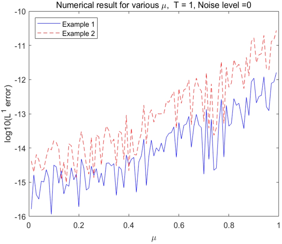
Figure 1 illustrate the numerical errors of scheme (25) for and with various order μ (from 0.01 to 0.99 with step 0.01) when .
It can be seen from Fig. 1 that the numerical scheme (25) of Caputo fractional derivative is of high resolution for data without any noise.
Numerical error under with . Solid line is for and the dashed line for .
Numerical error under with various noise level . Solid line is for and the dashed line for .
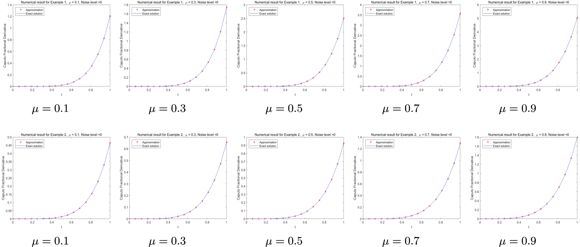
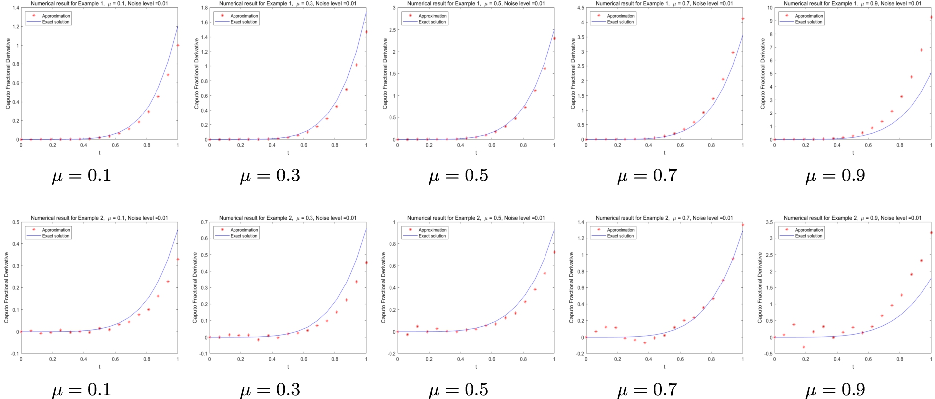
Numerical results for various order μ with noise level . The first row is for Example 1 and the second row for Example 2.
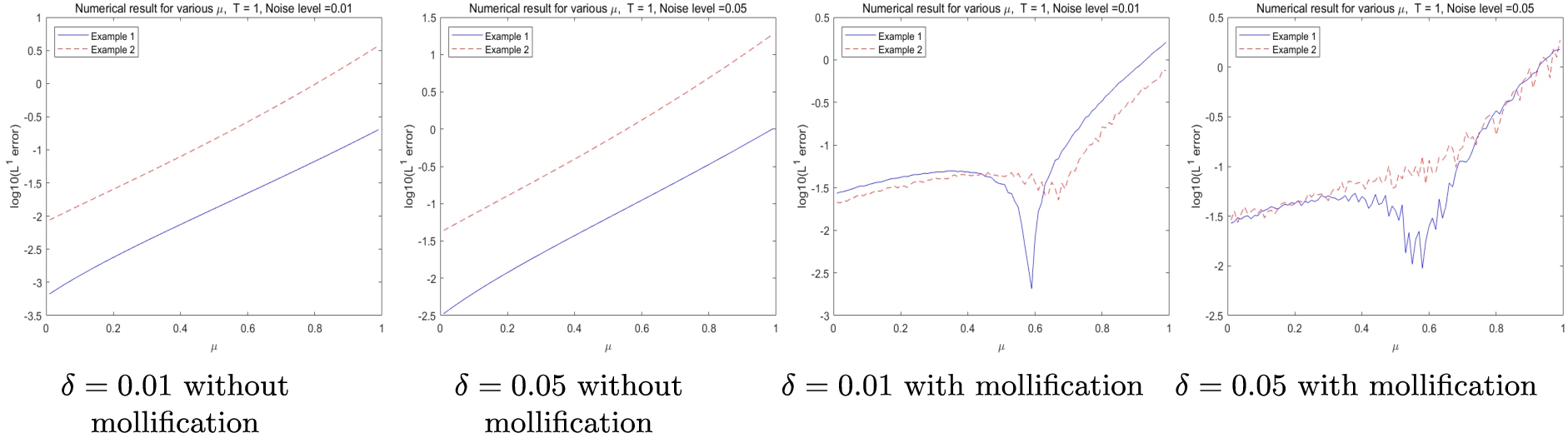
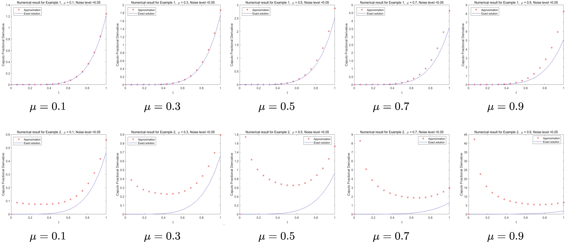
Numerical results for various order μ with noise level without mollification. The first row is for Example 1 and the second row for Example 2.
Numerical results for various order μ with noise level with mollification. The first row is for Example 1 and the second row for Example 2.
Numerical results for various order μ with noise level without mollification. The first row is for Example 1 and the second row for Example 2.
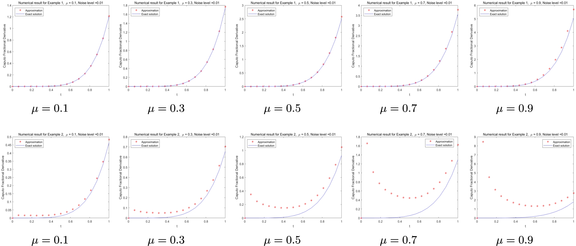
Figures 1 and 3 show that the scheme (26) performs excellent to calculate the fractional derivative numerically for various order under the data without any noise. Figures 2 exhibit that the effect of numerical scheme with mollification regularization under various fractional order (from 0.01 to 0.99) is significantly better than the case without mollification when data contains noise. Figures 4 and 5 illustrate a comparison of numerical fractional derivative for diverse order without- and with- mollification method under the noise level , and the corresponding results for noise level are elaborated in Fig. 6 and Fig. 7. The above figures state the truth that the numerical algorithm performs overwhelmingly well as data is exactly, and the mollification regularization method helps the numerical scheme achieve an effective solution when data contains noise. The experimental results are in good agreement with the theoretical results.
Conclusion
We propose a numerical scheme to approximate Caputo fractional derivative with order by using Jacobi–Gauss–Lobatto collocation method on the sense of Gaussian quadrature, and the convergence analysis is presented as well. Some numerical experiments well verified the theoretical results, and confirmed the efficiency to approximate fractional derivative by invoking mollification as function data comprises noise. The proposed method provides a versatile and effective approach to calculate the fractional derivative. The same technique can be extend to other quadrature rules which include one endpoint or all interior points.
Footnotes
Acknowledgements
The authors would like to thank editors and reviewers for their valuable suggestions and comments. This work is partially supported by National Natural Science Foundation of China (11861007, 11961002, 12061008, 12261004), Natural Science Foundation of Jiangxi Province of China (20232BAB201019).
Conflict of interest
We declare that we do not have any commercial or associative interest that represents a conflict of interest in connection with the work submitted.
References
1.
C.Canuto, M.Y.Hussaini, A.Quarteroni and T.A.Zang, Spectral Methods. Fundamentals in Single Domains, Springer-Verlag, Berlin, 2006.
2.
A.Carpinteri and F.Mainardi, Fractals and Fractional Calculus in Continuum Mechanics, Springer-Verlag, Vienna, 1998.
3.
S.Chen, J.Shen and L.L.Wang, Generalized Jacobi functions and their applications to fractional differential equations, Mathematics of Computation85(300) (2016), 1603–1638. doi:10.1090/mcom3035.
4.
S.Chen, J.Shen, Z.M.Zhang and Z.Zhou, A spectrally accurate approximation to subdiffusion equations using the log orthogonal functions, SIAM Journal on Scientific Computing42(2) (2020), A849–A877. doi:10.1137/19M1281927.
5.
W.Chester, Resonant oscillations in closed tubes, Journal of Fluid Mechanics18(1) (1964), 44–64. doi:10.1017/S0022112064000040.
S.Esmaeili and G.V.Milovanović, Nonstandard Gauss–Lobatto quadrature approximation to fractional derivatives, Fractional Calculus and Applied Analysis17(4) (2014), 1075–1099. doi:10.2478/s13540-014-0215-z.
8.
B.Y.Guo and L.L.Wang, Jacobi interpolation approximations and their applications to singular differential equations, Advances in Computational Mathematics14 (2001), 227–276. doi:10.1023/A:1016681018268.
9.
B.Y.Guo and L.L.Wang, Jacobi approximations in non-uniformly Jacobi-weighted Sobolev spaces, Journal of Approximation Theory128(1) (2004), 1–41. doi:10.1016/j.jat.2004.03.008.
10.
J.Hesthaven, S.Gottlieb and D.Gottlieb, Spectral Methods for Time-Dependent Problems, Cambridge University Press, Cambridge, 2007.
11.
B.T.Jin and Z.Zhou, Recovery of a space-time-dependent diffusion coefficient in subdiffusion: Stability, approximation and error analysis, IMA Journal of Numerical Analysisdrac051 (2022).
12.
J.J.Keller, Propagation of simple non-linear waves in gas filled tubes with friction, Z. angew. Math. Phys.32 (1981), 170–181. doi:10.1007/BF00946746.
13.
Y.M.Lin and C.J.Xu, Finite difference/spectral approximations for the time-fractional diffusion equation, Journal of Computational Physics225(2) (2007), 1533–1552. doi:10.1016/j.jcp.2007.02.001.
14.
R.L.Magin, Fractional Calculus in Bioengineering, Begell House Inc., Redding, 2006.
15.
Z.P.Mao and G.E.Karniadakis, A spectral method (of exponential convergence) for singular solutions of the diffusion equation with general two-sided fractional derivative, SIAM Journal on Numerical Analysis56 (2018), 24–49. doi:10.1137/16M1103622.
16.
G.Mastroianni and D.Occorsio, Optimal systems of nodes for Lagrange interpolation on bounded intervals. A survey, Journal of Computational and Applied Mathematics134 (2001), 325–341. doi:10.1016/S0377-0427(00)00557-4.
17.
D.A.Murio, On the stable numerical evaluation of Caputo fractional derivatives, Computers & Mathematics with Applications51(9–10) (2006), 1539–1550. doi:10.1016/j.camwa.2005.11.037.
18.
D.X.Nie, J.Sun and W.H.Deng, Sharp error estimates for spatial-temporal finite difference approximations to fractional sub-diffusion equation without regularity assumption on the exact solution, Fractional Calculus and Applied Analysis26 (2023), 1421–1464. doi:10.1007/s13540-023-00162-3.
19.
I.Podlubny, Fractional Differential Equations, Academic Press, San Diego, 1999.
20.
J.Shen, T.Tang and L.L.Wang, Spectral Methods: Algorithms, Analysis and Applications, Springer-Verlag, Berlin Heidelberg, 2011.
21.
N.Sugimoto and T.Kakutani, Generalized Burgers’ equation for nonlinear viscoelastic waves, Wave Motion7(5) (1985), 447–458. doi:10.1016/0165-2125(85)90019-8.
22.
B.J.West, M.Bologna and P.Grigolini, Physics of Fractal Operators, Springer-Verlag, New York, 2003.
23.
M.Zayernouri and G.E.Karniadakis, Fractional Sturm–Liouville eigen-problems: Theory and numerical approximation, Journal of Computational Physics252 (2013), 495–517. doi:10.1016/j.jcp.2013.06.031.
24.
M.Zayernouri and G.E.Karniadakis, Fractional spectral collocation method, SIAM Journal on Scientific Computing36(1) (2014), A40–A62. doi:10.1137/130933216.
25.
M.Zayernouri and G.E.Karniadakis, Fractional spectral collocation methods for linear and nonlinear variable order FPDEs, Journal of Computational Physics293 (2015), 312–338. doi:10.1016/j.jcp.2014.12.001.