Sage Journals: Discover world-class research

Abstract

We analyze an approximate interior transmission eigenvalue problem in $R^{d}$ for $d = 2$ or $d = 3$ , motivated by the transmission problem of a transformation optics-based cloaking scheme and obtained by replacing the refractive index with its first order approximation, which is an unbounded function. Using the radial symmetry we show the existence of (infinitely many) complex transmission eigenvalues and prove their discreteness. Moreover, it is shown that there exists a horizontal strip in the complex plane around the real axis, that does not contain any transmission eigenvalues.

Keywords

Born approximation transmission eigenvalues eigenvalue-free regions inverse scattering spherically stratified medium

1. Introduction

Transmission eigenvalue problems have become an important area of research in inverse scattering theory. We refer the reader to [4] for a recent survey article, or to [5,12] and the references therein. The relation of transmission eigenvalues to cloaking, or to so-called non-scattering wave numbers is noteworthy [2,9,10,17,41]. At such wave numbers there exists an incident field which does not scatter, i.e. the obstacle becomes invisible, when probed by that incident field. In [7] we considered an approximate, transformation optics-based cloaking scheme for the Helmholtz equation that incorporated a Drude–Lorentz model [21,30] to account for the dispersive properties of the cloak. Specifically, the goal is to make $B_{1}$ , the ball of radius 1 centered at the origin, approximately invisible to a far observer, independently of its contents. This is done using ideas from transformation optics [18,19,25,26,35,37,38] by surrounding the cloaked region $B_{1}$ with a layer of an appropriate anisotropic material that we assume occupies the annulus $B_{2} ∖ B_{1}$ and refer to it as the cloak, or the cloaking layer. The material properties of the cloak are obtained via change of variables using a map $F_{ϵ}$ that blows up a small ball $B_{ϵ}$ of radius $ϵ > 0$ to the cloaked region $B_{1}$ , while keeping the outer boundary $\partial B_{2}$ fixed (this map is commonly used in many cloaking papers, e.g. [25,26,30], but its precise formula is irrelevant here). Finally, by including a layer of extremely high conductivity adjacent to $B_{1}$ , without loss of generality we assume that $B_{1}$ is “soft”, i.e. we impose a zero Dirichlet boundary condition on $\partial B_{1}$ . The refractive index of this cloak is $\begin{aligned} (1.1) & n_{ϵ} (x, k) = 1 + σ_{ϵ} (k) det D F_{ϵ} (x), \end{aligned}$ where $\begin{array}{r} σ_{ϵ} (k) = \frac{1}{k_{ϵ}^{2} - k^{2} - i k} and det D F_{ϵ} (x) = \frac{{(2 - 2 ϵ + | x |)}^{d - 1}}{{(2 - ϵ)}^{d} | x |^{d - 1}} . \end{array}$

Here k denotes the wave number, $d = 2$ or $d = 3$ is the dimension and $k_{ϵ} > 0$ represents the so-called resonant frequency of the Drude–Lorentz term. The interior transmission eigenvalue problem corresponding to this cloaking scheme is nonlinear and its complete analysis is an open problem: the existing approaches do not apply [5]. It turns out [7] that there are no real transmission eigenvalues, consequently perfect cloaking/non-scattering is impossible at any $k > 0$ . However, one can achieve approximate cloaking: under certain growth assumption on $k_{ϵ}$ , the scattered field of the cloak and its far field pattern can be made uniformly small (of order ϵ in 3d and $1 / | ln ϵ |$ in 2d) on any finite band of wave numbers and any incident field, provided ϵ is sufficiently small. Consistent with this growth assumption we will suppose that $\begin{array}{r} k_{ϵ}^{2} \sim ϵ^{- d}, ϵ \to 0 . \end{array}$

Interestingly, transmission eigenvalues exhibit non-discreteness: supported with numerical evidence, we conjectured that sequences of complex transmission eigenvalues accumulate at two finite points in the complex plane, namely the poles of the Drude–Lorentz term $σ_{ϵ} (k)$ .

With the motivation to have a better insight into the structure of this nonlinear transmission eigenvalue problem, in this paper we study a related Born transmission eigenvalue (BTE) problem. To be more precise, we note that for any fixed k one can expand $\begin{aligned} (1.2) & n_{ϵ} (x, k) = 1 + ϵ^{d} [m (x) + o (1)], \end{aligned}$ where the error term $o (1)$ converges to zero, as $ϵ \to 0$ pointwise in $x \neq 0$ (as well as in $L^{p} (B_{2})$ for suitable p), and m is given by $\begin{aligned} (1.3) & m (x) = m (| x |) = \frac{{(2 + | x |)}^{d - 1}}{2^{d} | x |^{d - 1}} . \end{aligned}$

Broadly speaking, in the weak scattering regime, or when the contrast of an obstacle is small, i.e. $n (x) = 1 + ϵ m (x)$ , where n denotes the refractive index of the scattering obstacle and $ϵ ≪ 1$ is a small parameter, the Born approximation to the scattered field $u^{s}$ is given by $\partial_{ϵ} u^{s} |_{ϵ = 0}$ (also, the Born approximation replaces the far filed operator by an operator that depends linearly on m, cf. [15]). For a background on the Born approximation and inverse scattering theory in the Born regime we refer to [6,22–24,29]. From the cloaking perspective, existence of real BTEs would imply better or higher order invisibility results at those wave numbers. Also, given the non-discreteness phenomenon in the interior transmission eigenvalue problem, one can wonder about non-discreteness in the corresponding Born problem. We address these questions and answer them negatively for the function m given by (1.3). We mention that it is a common assumption in the literature for the refractive index to be a bounded function, however, here $m \notin L^{\infty} (B_{2})$ .

The fact that there are no real BTEs is a well-known consequence of positivity of m [6,15]. The existence of countably many BTEs is obtained by making use of the radial geometry and following [6]: separating the variables, BTEs are described as zeros of a family of analytic functions. Another important, but harder question is about the location of the transmission eigenvalues in the complex plane. Specifically, it is useful to obtain information about eigenvalue free regions. The so-called linear sampling method [3,8,11] provides a technique to obtain qualitative information about the location and the shape of the scattering obstacle, from the scattered far field data. For justification of the linear sampling method in the time domain, the questions of discreteness and location of eigenvalues (relative to the real axis) are essential. With this in mind, we show that BTEs stay away from the real axis, i.e. there exists a strip in the complex plane, parallel to and containing the real axis, which does not contain any Born transmission eigenvalues. This will allow one to use the Fourier–Laplace transform and consider the time-domain linear sampling method [8]. Moreover, we also conjecture that any strip parallel to the real axis contains at most finitely many BTEs. For simplicity of presentation we carry out the proof for the function m given by (1.3). However, our methods apply to general positive and radial functions m for which $t^{d - 1} m (t)$ extends to a holomorphic function around the interval $[0, 2]$ , where t denotes the radial variable (cf. Remark 2.5).

Questions regarding the distribution of transmission eigenvalues in the complex plane, such as eigenvalue free regions were studied in [13,14,28,36,39,40]. However, there are not many works in this direction for BTEs. For example, in [6] among other things, the authors study the distribution of those BTEs that correspond to radially symmetric eigenfunctions. One of the consequences of [36] is that (for the ball with constant refractive index) all transmission eigenvalues lie in a horizontal strip containing the real axis. Our work exhibits qualitative difference between the distributions of transmission eigenvalues (TEs) and those in the Born regime (BTEs), it shows somewhat contrary, or dual behavior of BTEs, namely that all of them lie outside of some horizontal strip around the real axis. Or, invoking the conjectured stronger statement, all (but possibly finitely many) BTEs lie outside of any horizontal strip. Our proof uses Olver’s uniform asymptotic expansion of Bessel functions of large order in the complex plane in terms of Airy functions [32–34]. We also use contour deformations and Mellin transform techniques [42].

2. The main result

The transmission eigenvalue (TE) problem corresponding to the cloaking scheme described in the introduction is anisotropic, however changing the variables in the transmitted field inside the cloak using the map $F_{ϵ}$ and leaving the incident field unchanged, one can get rid of the anisotopy. As a result we arrive at the following equivalent TE problem in $R^{d}$ for $d = 2$ or $d = 3$ (cf. (4.1) in [7]): $\begin{aligned} (2.1) & \{\begin{array}{ll} Δ u + k^{2} n_{ϵ} (\cdot, k) u = 0, & in B_{2} ∖ {\overline{B}}_{ϵ} \\ Δ v + k^{2} v = 0, & in B_{2} \\ u = v, & on \partial B_{2} \\ \partial_{ν} u = \partial_{ν} v & on \partial B_{2} \\ u = 0, & on \partial B_{ϵ}, \end{array} \end{aligned}$ where $n_{ϵ}$ is given by (1.1). Assume the function u from (2.1) can be approximated by $u \approx u_{0} + ϵ^{d} u_{1}$ , where $u_{0}, u_{1}$ are defined in $B_{2}$ . When v is of the same order as $u_{0}$ , for $u_{1}$ we consider the following approximation (for scattering estimates from a small circular obstacle we refer to, e.g. [20]) $\begin{aligned} (2.2) & \{\begin{array}{ll} Δ u + k^{2} u = - k^{2} m v, & in B_{2} \\ Δ v + k^{2} v = 0, & in B_{2} \\ u = \partial_{ν} u = 0, & on \partial B_{2}, \end{array} \end{aligned}$ where m is given by (1.3) and with abuse of notation we dropped the subscript from $u_{1}$ and still called this function u.

Definition 2.1.
$k \in C ∖ {0}$ is called a Born transmission eigenvalue (BTE) if there exists a nontrivial solution $u, v$ to (2.2), such that $u \in H^{2}$ and $m v \in L^{2}$ , where we suppress the domain $B_{2}$ from the notation of the function spaces.

Some remarks are now in order:
Remark 2.2.
∙ Note that when we formally take limits in (2.1), the equation for $u_{1}$ holds in the punctured ball $B_{2} ∖ {0}$ . Apriori $u_{1}$ may have a singularity at the origin and it might be interesting to consider families of interior transmission problems where the equation for $u_{1}$ holds in the punctured ball and has a prescribed singularity at the origin. This work is not concerned with the mathematical justification of the limiting procedure leading to (2.2). We assume that $u_{1}$ is regular at the origin and its equation is satisfied in $B_{2}$ .

∙ Due to the singularity of m there are no eigenvalues of (2.2) in the radially symmetric case. Indeed, say $d = 2$ and v is radial, then up to a multiplicative constant $v (x) = J_{0} (k | x |)$ , where $J_{0}$ is the Bessel function of order 0. As $J_{0}$ is regular near the origin we see that $m v \notin L^{2}$ due to the singularity of m. However, note that $\sqrt{m} v \in L^{2}$ . Therefore, this issue can be remedied by requiring $u, v$ to lie in the weighted spaces $H_{0, \frac{1}{m}}^{2}$ and $L_{m}^{2}$ , respectively (see also Remark 3.2 in Section 3). Where the notation means that $\sqrt{m} v \in L^{2}$ and $\frac{1}{\sqrt{m}} \partial^{α} u \in L^{2}$ for any multiindex $| α | ⩽ 2$ . The distribution of BTEs in the radially symmetric case was considered in [6] (for nonsingular m) and in this case BTEs are zeros of a single entire function. In this work BTEs are zeros of a countable family of entire functions and consequently analyzing their distribution in the complex plane is much more technical.

∙ It would be interesting to consider transmission eigenvalue problems like (2.2) in general domains with general singular weights m and analyze their solutions in the weighted Sobolev spaces mentioned above. This will be a task for the future.

The goal of this paper is to analyze the Born transmission eigenvalue problem (2.2). We point out that our core contribution is establishing part (iv) of the next theorem.
Theorem 2.3.
Let $d = 2$ or $d = 3$ , and m be given by ( 1.3 ). The following are true for the Born transmission eigenvalue problem ( 2.2 ):
There are no real, or purely imaginary BTEs.

There are infinitely many BTEs in $C ∖ (R \cup i R)$ .

BTEs form a discrete set in $C$ (i.e. a countable set with no limit points in $C$ ).

There exists $c > 0$ , such that there are no BTEs in the strip ${k \in C : | Im k | < c}$ .

Conjecture 2.4.
For any $C > 0$ , the strip ${k \in C : | Im k | < C}$ contains at most finitely many BTEs.
Remark 2.5.
Our methods of analysis for part (iv) apply to any positive and radially symmetric function $m = m (t)$ , where $t = | x |$ denotes the radial variable, for which $t^{d - 1} m (t)$ extends to a holomorphic function in some open set containing the interval $[0, 2]$ . In particular (also in view of Remark 3.2 in Section 3), our results can be applied to classical Born transmission eigenvalue problems (2.2) with non-singular (bounded) m.

The starting point in proving the above theorem is to use the radial symmetry and separation of variables, as in [6] to characterize BTEs as zeros of a countable family of entire functions ${B_{n} (k)}_{n = 1}^{\infty}$ . These functions are defined as integrals of the Bessel function (or its spherical counterpart for $d = 3$ ) of the first kind and order n, against an explicit function involving m (cf. Lemma 3.1). The first three items of Theorem 2.3 are proved using basic asymptotic approximations of Bessel functions. Item (iv) is significantly harder to prove and relies on Olver’s asymptotic formulas that exhibit the fine behaviour of the Bessel functions. Let us now outline the main idea behind proving the item (iv). We proceed by contradiction and assume that there exists a sequence ${k_{j}}_{j = 1}^{\infty} \subset C$ of distinct BTEs approaching the real line, i.e. $Im k_{j} \to 0$ , as $j \to \infty$ . Clearly, $B_{n_{j}} (k_{j}) = 0$ for some integer $n_{j}$ and all j. Using standard approximations and estimates of Bessel functions we first show that for each fixed n, the function $B_{n} (k)$ cannot have a sequence of distinct zeros lying in any horizontal strip in the complex plane. This allows us to conclude that $n_{j} \to \infty$ . The discreteness of BTEs (part (iii) of Theorem 2.3), on the other hand implies that $Re k_{j} \to \infty$ . We then find an explicit expression $E (n_{j}, k_{j})$ such that, upon passing to a subsequence if necessary, which we do not relabel, $\begin{aligned} (2.3) & | E (n_{j}, k_{j}) B_{n_{j}} (k_{j}) | ⩾ C \end{aligned}$ for some $C > 0$ and all j large enough. This provides the desired contradiction. The behavior of $B_{n_{j}} (k_{j})$ , or the explicit expression of $E (n_{j}, k_{j})$ depends on the growth of ${n_{j}}$ relative to ${k_{j}}$ . There are three different regimes, depending on whether one of these sequences grows at a rate comparable to, much faster or slower than the other one. The most delicate regime is arguably when the two sequences grow at a comparable rate. Special attention is given to the case where $k_{j} / n_{j} \to 1$ . This delicate behavior is due to the so-called turning point of the Bessel’s differential equation [34] at the point 1.
3. Discreteness and existence of the Born transmission eigenvalues

Here we prove items $(i)$ – $(i i i)$ of Theorem 2.3. We start by describing BTEs as zeros of a family of entire functions. This can be achieved by using the radial symmetry and separating the variables as is done in Theorem 1 of [6]. We omit the details and just state the result, as the proof is completely analogous. Throughout this paper, $J_{n}$ and $j_{n}$ denote the Bessel and spherical Bessel functions, respectively, of the first kind and order n. Recall that $\begin{aligned} (3.1) & j_{n} (z) = \sqrt{\frac{π}{2 z}} J_{n + \frac{1}{2}} (z) . \end{aligned}$

Lemma 3.1.
For $n = 1, 2$ ... introduce the functions $\begin{aligned} (3.2) & B_{n} (k) = \{\begin{array}{ll} \int_{0}^{1} f (t) J_{n}^{2} (k t) d t, & d = 2 \\ \int_{0}^{1} f (t) j_{n}^{2} (k t) d t, & d = 3, \end{array} \end{aligned}$ where $\begin{aligned} (3.3) & f (t) = \{\begin{array}{ll} 4 t m (2 t), & d = 2 \\ 8 t^{2} m (2 t), & d = 3 \end{array} = \{\begin{array}{ll} t + 1, & d = 2 \\ {(t + 1)}^{2}, & d = 3 . \end{array} \end{aligned}$

The set of zeros $\begin{array}{r} {k \in C ∖ {0} : B_{n} (k) = 0 for some n} \end{array}$ coincides with the set of BTEs for ( 2.2 ).
Remark 3.2.
In the radially symmetric case $n = 0$ and if we allow the eigenfunctions $u, v$ to lie in the weighted spaces $H_{0, \frac{1}{m}}^{2}$ and $L_{m}^{2}$ , respectively (as discussed in Remark 2.2), then the zeros of the function $B_{0}$ will also be eigenvalues. Therefore, throughout this paper we study the functions ${B_{n}}$ including the index $n = 0$ .

Next we collect some basic properties of the functions $B_{n}$ .
Lemma 3.3.
Let $n ⩾ 0$ be an integer and $B_{n} (k)$ be given by ( 3.2 ). Then
$B_{n} (k)$ is an entire function that has infinitely many zeros in $C$ and it has no real, or purely imaginary zeroes (apart possibly from $k = 0$ ).

$\overline{B_{n} (k)} = B_{n} (- \overline{k})$ .

$B_{n} \to 0$ , as $n \to \infty$ uniformly on compact subsets of $C$ .

Let ${k_{j}}_{j = 1}^{\infty} \subset C$ be a sequence of distinct zeros of $B_{n} (k)$ , for some fixed n, then $| Im k_{j} | \to \infty$ as $j \to \infty$ .

To prove the existence of infinitely many zeros of $B_{n}$ and the item (iv) of the above lemma, we borrow some ideas from Theorems 2 and 3 of [6]. The proof of Lemma 3.3 is given in Appendix A.1.

Note that the above two lemmas directly imply items (i) and (ii) of Theorem 2.3. Now we turn to proving item (iii) of Theorem 2.3. Lemma 3.4 (Discreteness).

Let $B_{n} (k)$ be given by ( 3.2 ), then the set ${k \in C : B_{n} (k) = 0 for some n ⩾ 0}$ is discrete in $C$ , i.e. it is a countable set with no limit points in $C$ .

Proof.
We give the proof for $d = 2$ , as for $d = 3$ the argument is analogous. Assume, for the sake of a contradiction that $k \in C$ is a limit point of the set of zeros of ${B_{n}}$ , let ${k_{j}}$ be a sequence of distinct points such that $B_{n_{j}} (k_{j}) = 0$ for some $n_{j} ⩾ 0$ , all $j ⩾ 1$ and $k_{j} \to k$ . Let us assume that $k_{j} \neq 0$ for all j. If ${n_{j}}$ stays bounded, then ${k_{j}}$ is a sequence of zeros of finitely many ${B_{n_{j}}}$ and upon passing to a subsequence ${k_{j}^{'}} \subset {k_{j}}$ , for some fixed integer $n_{0}$ we have $B_{n_{0}} (k_{j}^{'}) = 0$ for all j. Since $B_{n_{0}}$ is an entire function we conclude that $B_{n_{0}} \equiv 0$ , which is a contradiction. Thus, we may assume $n_{j} \to \infty$ .

We will use the large order asymptotic expansion of the Bessel function (cf. 9.3.1 of [1]): as $n \to \infty$ $\begin{aligned} (3.4) & J_{n} (z) \sim \frac{1}{\sqrt{2 π n}} {(\frac{e z}{2 n})}^{n}, \end{aligned}$ which holds uniformly for $z \in C$ bounded. In our case $z = k_{j} t$ stays bounded uniformly for j and $t \in [0, 1]$ . Consequently, as $j \to \infty$ $\begin{array}{r} B_{n_{j}} (k_{j}) \sim \frac{1}{2 π n_{j}} {(\frac{e k_{j}}{2 n_{j}})}^{2 n_{j}} \int_{0}^{1} t^{2 n_{j}} f (t) d t . \end{array}$

Therefore, for j large enough $\begin{array}{r} | B_{n_{j}} (k_{j}) | ⩾ \frac{1}{4 π n_{j}} {(\frac{e | k_{j} |}{2 n_{j}})}^{2 n_{j}} \int_{0}^{1} t^{2 n_{j}} f (t) d t, \end{array}$ which provides the desired contradiction, as the expression on the right hand side is positive: $f (t) > 0$ for all $t \in (0, 1)$ . □

4. The Born transmission eigenvalues and the real line

The goal of this section is to establish item (iv) of Theorem 2.3. Let us introduce $\begin{aligned} (4.1) & α (z) = ln (\frac{1 + \sqrt{1 - z^{2}}}{z}) - \sqrt{1 - z^{2}}, β (z) = \sqrt{z^{2} - 1} - arccos (z^{- 1}), \end{aligned}$ where all the functions are defined by their principal branches. Let also $\begin{aligned} (4.2) & V_{0} = {z \in C : 0 < Re z < 1}, V_{1} = {z \in C : Re z > 1} . \end{aligned}$

We remark that α is analytic in ${Re z > 0} ∖ [1, \infty)$ , while β in ${Re z > 0} ∖ (0, 1]$ . These functions show up in the uniform asymptotic expansion of Bessel functions of large order as stated in the lemma below.

Lemma 4.1.
Let $ν \in R$ , $ϵ \in (0, 1)$ and assume the notation introduced above. As $ν \to \infty$ , $\begin{aligned} (4.3) & J_{ν}^{2} (ν z) \sim \frac{1}{2 π ν \sqrt{1 - z^{2}}} e^{- 2 ν α (z)}, \end{aligned}$ uniformly for $z \in V_{0}$ with $| z | < 1 - ϵ$ .

Let now ${z_{ν}} \in V_{1}$ be a sequence with $| z_{ν} | > 1 + ϵ$ and $\begin{aligned} (4.4) & ν | Im z_{ν} | ⩽ c, \end{aligned}$ for all ν large enough and some constant $c > 0$ independent of ν. Then, as $ν \to \infty$ $\begin{aligned} (4.5) & J_{ν}^{2} (ν z_{ν}) = \frac{2}{π ν \sqrt{z_{ν}^{2} - 1}} [{cos}^{2} (ν β (z_{ν}) - \frac{π}{4}) + O (\frac{1}{ν})], \end{aligned}$ where the implicit constant in O depends only on ϵ and c.

The above lemma directly follows from the uniform asymptotic formulas of Bessel functions due to Olver. Specifically we first use the formulas 9.3.35–9.3.42 of [1] to expand $J_{n}$ in terms of the Airy function and its derivative (see also (A.13) in the Appendix, where this expansion is written down for future use). We then use the large argument asymptotics of the Airy function and its derivative ([1] 10.4.59 and 10.4.61) in the sector away from the real negative semiaxis. This yields the formula (4.3). To obtain (4.5) we use the asymptotics of Airy functions ([1] 10.4.60 and 10.4.62) in the sector containing the real negative semiaxis. The error bound in (4.5) follows from Theorem B of [33].

With these preliminaries, let us start the proof of part (iv) of Theorem 2.3. For the sake of contradiction, assume that there exists a sequence ${k_{j}}_{j = 1}^{\infty} \subset C$ of distinct BTEs, such that $Im k_{j} \to 0$ , as $j \to \infty$ .
Notation 4.2.
Unless stated otherwise, for the remainder of this section (including all the subsections) the limit and asymptotic relations are understood as $j \to \infty$ .

For each $k_{j}$ there exists an integer $n_{j} ⩾ 0$ with $B_{n_{j}} (k_{j}) = 0$ . If ${n_{j}}$ stays bounded, upon passing to a subsequence, which we do not relabel, $B_{n_{0}} (k_{j}) = 0$ for all $j ⩾ 1$ and some fixed integer $n_{0}$ . But item (iv) of Lemma 3.3 implies that ${k_{j}}$ cannot lie in any horizontal strip, which contradicts the boundedness of ${Im k_{j}}$ .

Thus, we may assume $n_{j} \to \infty$ . Further, if ${Re k_{j}}$ stays bounded, passing to a subsequence one concludes that BTEs have a limit point in $C$ , which cannot happen due to their discreteness as established in part (iii) of Theorem 2.3. Therefore, ${Re k_{j}}$ is unbounded and as BTEs are symmetric about the imaginary axis, we restrict our analysis to the right half-plane and assume that $Re k_{j} \to + \infty$ . To summarize we have: $\begin{aligned} (4.6) & n_{j} \to \infty, Re k_{j} \to + \infty, and Im k_{j} \to 0 . \end{aligned}$

As described in Section 2, to achieve the desired contradiction our goal will be to establish a lower bound on $B_{n_{j}} (k_{j})$ of the form (2.3). The behavior of $B_{n_{j}} (k_{j})$ is quite delicate and depends on the growth rate of the sequence ${n_{j}}$ relative to ${k_{j}}$ . There are three main regimes: $\begin{aligned} (4.7) & \begin{aligned} Case I: & n_{j} ≫ | k_{j} | \\ Case II: & n_{j} ≪ | k_{j} | \\ Case III: & k_{j} / n_{j} \to L, for some L > 0 and one of the following holds true: \\ a. & L < 1 \\ b. & L > 1 \\ c. & L = 1 \end{aligned} \end{aligned}$

In each of these regimes the behavior of $B_{n_{j}} (k_{j})$ is different. Further, in the subcase $L = 1$ , it even depends on the rate of convergence of $k_{j} / n_{j}$ to $L = 1$ . Before outlining the main ideas, let us first show that the above cases are exhaustive for our purposes. Indeed, our desired contradiction will be obtained if a lower bound of form (2.3) is established for some subsequences of ${n_{j}}$ and ${k_{j}}$ . In other words, we can pass to subsequences when necessary. Now, if Case II is not satisfied, then $k_{j} / n_{j}$ has a bounded subsequence. Passing to a further subsequence, without relabeling it, we may assume $k_{j} / n_{j} \to L$ , for some $L \in C$ . Due to (4.6), $L ⩾ 0$ . If $L = 0$ , then Case I holds, otherwise: Case III.

Turning to the main ideas, we will present all the proofs when $d = 2$ , as $d = 3$ is completely analogous due to the relation (3.1) and we will only state the corresponding results with additional comments whenever necessary. Note that we can rewrite $\begin{aligned} (4.8) & B_{n_{j}} (k_{j}) = \int_{0}^{1} f (t) J_{n_{j}}^{2} (n_{j} z_{j} (t)) d t, z_{j} (t) = \frac{k_{j}}{n_{j}} t . \end{aligned}$

The idea is to use the asymptotic relations in Lemma 4.1 to replace $J_{n_{j}}^{2} (n_{j} z)$ with an appropriate expression. The behavior of $J_{n_{j}}^{2} (n_{j} z)$ , however, is very delicate near the so-called turning point $z = 1$ . Lemma 4.1 already demonstrates different behaviors depending on whether $z = z_{j} (t)$ lies to the left, or to the right of the line ${Re z = 1}$ and stays away from $z = 1$ (when it approaches $z = 1$ the behavior is quite complicated and depends on the convergence rate of $z_{j}$ to 1). Case I of (4.7) is the easiest to analyze, as $z = z_{j} (t)$ always stays away from $z = 1$ and lies to the left of ${Re z = 1}$ , therefore the asymptotic relation (4.3) can be readily used. The other two cases require more work. We split the integral in (4.8) into parts such that for each t in the respective integration region $z = z_{j} (t)$ stays away from $z = 1$ and either the relation (4.3) or (4.5) can be used. It is the integral, in which $z_{j} (t)$ can be arbitrarily close to $z = 1$ that needs special care. In Case II we use Mellin transforms to treat this integral. In Case III, apart from using Mellin transforms, we also use the asymptotic expansion of $J_{n_{j}}^{2} (n_{j} z)$ in terms of the Airy function and its derivative. The behavior of $B_{n_{j}} (k_{j})$ is then described in terms of the Airy function.

Case I is treated in Section 4.1, Case II in Section 4.2 and Case III in Section 4.3.
4.1. Case I: The regime $n_{j} ≫ | k_{j} |$

In (4.8) for j large enough $| z_{j} (t) | < 1 / 2$ uniformly for $t \in (0, 1)$ . Therefore, applying the first part of Lemma 4.1 and conclude that $\begin{aligned} (4.9) & B_{n_{j}} (k_{j}) \sim \frac{1}{2 π n_{j}} \int_{0}^{1} \frac{f (t)}{\sqrt{1 - z_{j} {(t)}^{2}}} e^{- 2 n_{j} α (z_{j} (t))} d t \sim \frac{1}{2 π n_{j}} \int_{0}^{1} f (t) e^{- 2 n_{j} α (z_{j} (t))} d t, \end{aligned}$ where in the second step we used that $z_{j} (t) \to 0$ uniformly in t. The function α given by (4.1), blows up near the origin, namely as $z \to 0$ from inside the right half-plane, $α (z) \sim ln (\frac{2}{z}) - 1$ . Therefore we introduce the function $\begin{aligned} (4.10) & \tilde{α} (z) = α (z) + 1 - ln \frac{2}{z} = 1 - \sqrt{1 - z^{2}} + ln \frac{1 + \sqrt{1 - z^{2}}}{2} . \end{aligned}$

It is straightforward to show that as $z \to 0$ from inside the right half-plane, $\tilde{α} (z) \sim \frac{z^{2}}{4}$ . In terms of the function $\tilde{α}$ , we can rewrite the asymptotics (4.9) as $\begin{aligned} B_{n_{j}} (k_{j}) & \sim \frac{1}{2 π n_{j}} {(\frac{k_{j} e}{2 n_{j}})}^{2 n_{j}} \int_{0}^{1} f (t) t^{2 n_{j}} e^{- 2 n_{j} \tilde{α} (z_{j} (t))} d t \\ \sim \frac{1}{{(n_{j}!)}^{2}} {(\frac{k_{j}}{2})}^{2 n_{j}} \int_{0}^{1} f (t) t^{2 n_{j}} e^{- 2 n_{j} \tilde{α} (z_{j} (t))} d t, \end{aligned}$ where we used the Stirling’s formula in the last step. We will prove below that for any z with $0 < Re z < 1$ and $| z | < C$ we have $\begin{aligned} (4.11) & | Im \tilde{α} (z) | ⩽ C | Im z | . \end{aligned}$

Applying this inequality, we conclude that for j large enough $\begin{array}{r} n_{j} | Im \tilde{α} (z_{j} (t)) | ⩽ t | Im k_{j} | ⩽ | Im k_{j} |, \end{array}$ which converges to zero as $j \to \infty$ uniformly in t, due to our assumption on ${k_{j}}$ (cf. (4.6)). Therefore, as $j \to \infty$ $\begin{array}{r} e^{- i 2 n_{j} Im \tilde{α} (z_{j} (t))} \to 1, \end{array}$ uniformly for $t \in (0, 1)$ . Consequently, $\begin{aligned} (4.12) & {(n_{j}!)}^{2} {(\frac{2}{k_{j}})}^{2 n_{j}} B_{n_{j}} (k_{j}) \sim \int_{0}^{1} f (t) t^{2 n_{j}} e^{- 2 n_{j} Re \tilde{α} (z_{j} (t))} d t . \end{aligned}$

The right hand side of the above asymptotic relation is real-valued and positive. This provides the desired contradiction.

Thus, to finish the proof it remains to establish (4.11). Let $| z | < 1 - ϵ$ for some small $ϵ > 0$ and $Re z > 0$ . We have the representation $\begin{array}{r} \tilde{α} (z) = \int_{0}^{z} \frac{ξ d ξ}{1 + \sqrt{1 - ξ^{2}}} = \int_{0}^{Re z} \frac{x d x}{1 + \sqrt{1 - x^{2}}} + \int_{Re z}^{z} \frac{ξ d ξ}{1 + \sqrt{1 - ξ^{2}}}, \end{array}$ where we chose the contour of integration to be the line segment joining 0 to $Re z$ , followed by the one joining $Re z$ to z. As the first integral in the above formula is real, it does not affect the imaginary part of $\tilde{α}$ . For the second integral $| 1 + \sqrt{1 - ξ^{2}} | ⩾ 1$ , which implies the desired bound $\begin{array}{r} | Im \tilde{α} (z) | ⩽ | z | \cdot | z - Re z | < (1 - ϵ) | Im z | . \end{array}$

4.2. Case II: The regime $n_{j} ≪ | k_{j} |$

Due to the relation (3.1) between the Bessel functions $j_{n}$ and $J_{n}$ , it is convenient to introduce the index notation $\begin{aligned} (4.13) & ν_{j} = \{\begin{array}{ll} n_{j}, & d = 2 \\ n_{j} + \frac{1}{2}, & d = 3 . \end{array} \end{aligned}$

We proceed by letting $d = 2$ . The above notation helps to treat the case $d = 3$ in parallel: when $d = 3$ , in what follows one just replaces $J_{n}$ with $j_{n}$ .

As already discussed in the paragraph below (4.8), we first split the integral defining $B_{n}$ , into parts where $z_{j} (t) = k_{j} t / n_{j}$ stays away from $z = 1$ . To that end, let us fix a small parameter $ϵ > 0$ and split $\begin{aligned} (4.14) & B_{n_{j}} (k_{j}) = \int_{0}^{(1 - ϵ) \frac{ν_{j}}{| k_{j} |}} + \int_{(1 - ϵ) \frac{ν_{j}}{| k_{j} |}}^{(1 + ϵ) \frac{ν_{j}}{| k_{j} |}} + \int_{(1 + ϵ) \frac{ν_{j}}{| k_{j} |}}^{1}, \end{aligned}$ where the integrand $f (t) J_{n_{j}}^{2} (k_{j} t) d t$ was suppressed from the notation. Note that in the first and third integrals $z_{j} (t)$ stays away from $z = 1$ , while in the second one it can get arbitrarily close to $z = 1$ . To analyze the second integral we first change the variables $\begin{aligned} (4.15) & \int_{(1 - ϵ) \frac{ν_{j}}{| k_{j} |}}^{(1 + ϵ) \frac{ν_{j}}{| k_{j} |}} f (t) J_{n_{j}}^{2} (k_{j} t) d t = \frac{ν_{j}}{k_{j}} \int_{(1 - ϵ) \frac{k_{j}}{| k_{j} |}}^{(1 + ϵ) \frac{k_{j}}{| k_{j} |}} f (\frac{ν_{j}}{k_{j}} z) J_{n_{j}}^{2} (ν_{j} z) d z, \end{aligned}$ where in the last integral we take the contour of integration to be the line segment connecting the two endpoints (in fact, it can be taken to be an arbitrary path, as the integrand is an entire function of z). Note that $k_{j} / | k_{j} | \to 1$ , due to our assumptions on $k_{j}$ (cf. (4.6)). Therefore, the contour of integration approaches to the interval $[1 - ϵ, 1 + ϵ]$ in the limit. Further, $k_{j} / | k_{j} | = e^{i arg k_{j}}$ simply rotates this interval and so the integral in (4.15) is over the line segment $P Q$ as shown in Fig. 1.

Fig. 1.

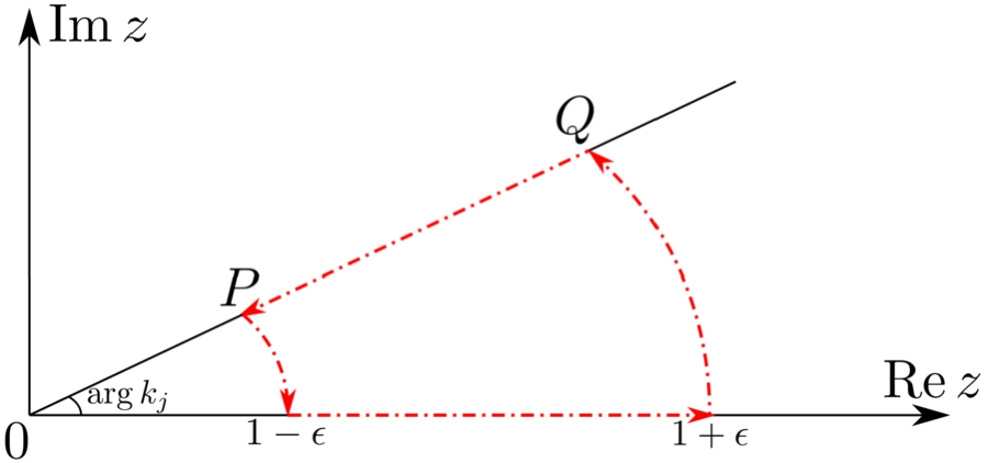
The contour of integration.

We are going to analyze the integral (4.15) via Mellin transform, however this technique does not work when z is complex (cf. Remark 4.7). Therefore, we first need to deform the integral of the analytic function $z \mapsto f (\frac{ν_{j}}{k_{j}} z) J_{n_{j}}^{2} (ν_{j} z)$ over $P Q$ to the integral over $[1 - ϵ, 1 + ϵ]$ , taking into account the two integrals over circular arcs as shown in Fig. 1. The integral over the circular arc joining P to $1 - ϵ$ will be grouped with the first integral in (4.14), while the integral over the other circular arc will be grouped with the second integral in (4.14). Putting things together we arrive at the following decomposition: $\begin{array}{r} B_{n_{j}} (k_{j}) = I_{1} + I_{2} + I_{3}, \end{array}$ where $\begin{aligned} (4.16) & \begin{aligned} I_{1} = & \int_{0}^{(1 - ϵ) \frac{ν_{j}}{| k_{j} |}} f (t) J_{n_{j}}^{2} (k_{j} t) d t \\ - i \frac{ν_{j}}{k_{j}} (1 - ϵ) \int_{0}^{arg k_{j}} f (\frac{ν_{j}}{k_{j}} (1 - ϵ) e^{i θ}) J_{n_{j}}^{2} (ν_{j} (1 - ϵ) e^{i θ}) e^{i θ} d θ, \\ I_{2} = & \int_{(1 + ϵ) \frac{ν_{j}}{| k_{j} |}}^{1} f (t) J_{n_{j}}^{2} (k_{j} t) d t \\ + i \frac{ν_{j}}{k_{j}} (1 + ϵ) \int_{0}^{arg k_{j}} f (\frac{ν_{j}}{k_{j}} (1 + ϵ) e^{i θ}) J_{n_{j}}^{2} (ν_{j} (1 + ϵ) e^{i θ}) e^{i θ} d θ \end{aligned} \end{aligned}$ and $\begin{aligned} (4.17) & I_{3} = \frac{ν_{j}}{k_{j}} \int_{1 - ϵ}^{1 + ϵ} f (\frac{ν_{j}}{k_{j}} t) J_{n_{j}}^{2} (ν_{j} t) d t . \end{aligned}$

Note that $I_{l} = I_{l} (n_{j}, k_{j}, ϵ)$ for $l = 1, 2, 3$ , but these dependencies will be suppressed for the ease of notation. The advantage of above decomposition is that in $I_{1}, I_{2}$ we can use the large order asymptotics of the Bessel function from Lemma 4.1 as z stays away from 1. While in $I_{3}$ , the integration variable is real and we can apply Mellin transform techniques. In the subsections below, we will show that $\begin{aligned} (4.18) & k_{j} I_{1} \to 0, I_{2} \sim \frac{ln (k_{j} / n_{j})}{π k_{j}}, k_{j} I_{3} \to c_{1}, \end{aligned}$ where $c_{1} = c_{1} (ϵ)$ is some constant (cf. (4.26)). These asymptotic relations in particular imply $\begin{array}{r} \frac{π k_{j}}{ln (k_{j} / n_{j})} B_{n_{j}} (k_{j}) \sim 1, \end{array}$ which yields the desired inequality of the form (2.3) and contradicts the fact that ${k_{j}}$ are zeros of $B_{n_{j}}$ .

Remark 4.3.

When $d = 3$ , the integrals $I_{l}$ for $l = 1, 2, 3$ are given by the same formulas as above, except with $j_{n}$ in place of $J_{n}$ . The asymptotic relations in this case take the form $\begin{array}{r} n_{j} k_{j} I_{1} \to 0, n_{j} k_{j} I_{2} \to \frac{1}{2} arctan \frac{1}{\sqrt{ϵ^{2} + 2 ϵ}}, n_{j} k_{j} I_{3} \to c_{2}, \end{array}$ where $c_{2} = c_{2} (ϵ)$ is a constant, such that $c_{2} (ϵ) \to 0$ as $ϵ \to 0$ (cf. (4.27)). These readily imply that $\begin{array}{r} lim_{j \to \infty} n_{j} k_{j} B_{n_{j}} (k_{j}) = \frac{1}{2} arctan \frac{1}{\sqrt{ϵ^{2} + 2 ϵ}} + c (ϵ) . \end{array}$

As the left hand side of the last expression does not depend on ϵ, we can take limits as $ϵ \to 0$ and conclude $\begin{array}{r} \frac{4}{π} n_{j} k_{j} B_{n_{j}} (k_{j}) \sim 1 . \end{array}$

4.2.1. Analyzing

I_{1}

via uniform asymptotics of the Bessel function

Let $I_{1}$ be given by (4.16) and $d = 2$ . Here we show the first relation of (4.18), i.e. $k_{j} I_{1} \to 0$ . In fact, we will see below that this convergence to zero is at an exponential rate with respect to $n_{j}$ . The formula of $I_{1}$ in (4.16) contains two integral terms, the first of which we denote by $I_{11}$ and the second one by $I_{12}$ , so that $\begin{array}{r} I_{1} = I_{11} + I_{12} . \end{array}$

We start by analyzing $I_{11}$ . Note that it can be rewritten as $\begin{array}{r} I_{11} = \int_{0}^{(1 - ϵ) \frac{n_{j}}{| k_{j} |}} f (t) J_{n_{j}}^{2} (n_{j} z_{j} (t)) d t, z_{j} (t) = \frac{k_{j}}{n_{j}} t . \end{array}$

For any t in the integration interval $\begin{aligned} (4.19) & | z_{j} (t) | ⩽ \frac{| k_{j} |}{n_{j}} t < 1 - ϵ \end{aligned}$ and $z_{j} (t)$ lies in the right half-plane, therefore the formula (4.3) of Lemma 4.1 can be used to obtain the asymptotics, as $j \to \infty$ , of the Bessel function in the integrand of $I_{11}$ , uniformly for t inside the integration interval. Hence, this asymptotic relation can be multiplied by $f (t)$ and integrated in t. This gives the asymptotic behavior of $I_{11}$ . Multiplying the latter by $k_{j}$ and taking absolute values we conclude that, as $j \to \infty$ $\begin{aligned} (4.20) & | k_{j} I_{11} | \sim \frac{| k_{j} |}{2 π n_{j}} | \int_{0}^{(1 - ϵ) \frac{n_{j}}{| k_{j} |}} \frac{f (t)}{\sqrt{1 - z_{j}^{2} (t)}} e^{- 2 n_{j} α (z_{j} (t))} d t | ⩽ \frac{C | k_{j} |}{ϵ n_{j}} \int_{0}^{(1 - ϵ) \frac{n_{j}}{| k_{j} |}} e^{- 2 n_{j} Re α (z_{j} (t))} d t, \end{aligned}$ where α is given by (4.1), C is an absolute constant and we used (4.19) to bound the square root term from below in the denominator of above integrand. Note that since ${Im k_{j}}$ is bounded, due to (4.6), $\begin{aligned} (4.21) & Im z_{j} (t) = \frac{Im k_{j}}{n_{j}} t \to 0, as j \to \infty \end{aligned}$ uniformly for t inside the integration interval. Next we need the following lower bound on α, which holds provided the imaginary part of its argument is sufficiently small (this is guaranteed by (4.21)): there exists $j_{0} > 0$ and $c = c_{ϵ} > 0$ , such that $\begin{array}{r} Re α (z_{j} (t)) ⩾ c, j ⩾ j_{0}, t \in (0, \frac{(1 - ϵ) n_{j}}{| k_{j} |}) . \end{array}$

This is a consequence of the explicit form of the function α and the proof can be found in part (ii) of Lemma A.1 in the Appendix (in fact, here we need the weaker version of the lower bound (A.18), where we drop the logarithm term. The stronger lower bound as formulated in (A.18) is needed in the case $d = 3$ ). Now, for large enough j, the right hand side of (4.20) can be bounded by $C_{ϵ} e^{- 2 n_{j} c_{ϵ}}$ , which converges to zero concluding the proof for $I_{11}$ .

Let us now turn to $I_{12}$ : $\begin{array}{r} I_{12} = - i \frac{n_{j}}{k_{j}} (1 - ϵ) \int_{0}^{arg k_{j}} f (\frac{n_{j}}{k_{j}} z (θ)) J_{n_{j}}^{2} (n_{j} z (θ)) e^{i θ} d θ, \end{array}$ where $z (θ) = (1 - ϵ) e^{i θ}$ does not depend on j. It has exactly the same properties as $z_{j} (t)$ above. The only difference from the above analysis is that the argument of f now depends on j, but note that it converges to 0 uniformly in θ, hence f can be replaced with $f (0)$ in the large j asymptotics. Therefore, $\begin{array}{r} | k_{j} I_{12} | \sim \frac{(1 - ϵ) | f (0) |}{2 π} | \int_{0}^{arg k_{j}} \frac{1}{\sqrt{1 - z^{2} (θ)}} e^{- 2 n_{j} α (z (θ))} d θ | . \end{array}$

As ${Im k_{j}}$ is bounded and $Re k_{j} \to + \infty$ we deduce that $arg k_{j} \to 0$ , so that $Im z (θ) = (1 - ϵ) sin θ$ is small for large j, uniformly for θ between 0 and $arg k_{j}$ . Therefore, the above lower bound on $Re α$ can be used again, yielding the same conclusion: $k_{j} I_{12} \to 0$ . Putting the estimates for $I_{11}$ and $I_{12}$ together, we conclude the proof.

4.2.2. Analyzing $I_{2}$ via uniform asymptotics of the Bessel function

Let $I_{2}$ be given by (4.16) and $d = 2$ . Here we prove the second relation of (4.18), i.e. $π k_{j} I_{2} \sim ln (k_{j} / n_{j})$ . The definition of $I_{2}$ in (4.16) contains two integral terms, the first of which we denote by $I_{21}$ and the second one by $I_{22}$ , so that $\begin{array}{r} I_{2} = I_{21} + I_{22} \end{array}$

The desired result will follow after showing $\begin{aligned} (4.22) & π k_{j} I_{21} \sim ln (k_{j} / n_{j}), k_{j} I_{22} \to 0 . \end{aligned}$

Remark 4.4.
When $d = 3$ , the corresponding results read $\begin{array}{r} 2 n_{j} k_{j} I_{21} \to arctan {(ϵ^{2} + 2 ϵ)}^{- \frac{1}{2}}, n_{j} k_{j} I_{22} \to 0 . \end{array}$

∙ We start from the term $I_{21}$ : $\begin{array}{r} I_{21} = \int_{(1 + ϵ) \frac{n_{j}}{| k_{j} |}}^{1} f (t) J_{n_{j}}^{2} (n_{j} z_{j} (t)) d t, z_{j} (t) = \frac{k_{j}}{n_{j}} t . \end{array}$

Note that for any t in the integration interval $| z_{j} (t) | > 1 + ϵ$ and $z_{j} (t)$ lies in the right half-plane. Further, $n_{j} | Im z_{j} (t) | ⩽ c$ for some $c > 0$ , as ${Im k_{j}}$ is bounded. Therefore, we can apply the asymptotic formula (4.5) of Lemma 4.1 for the Bessel function in the above integral, uniformly in t: $\begin{array}{r} I_{21} = \frac{2}{π n_{j}} \int_{(1 + ϵ) \frac{n_{j}}{| k_{j} |}}^{1} \frac{f (t)}{\sqrt{z_{j}^{2} (t) - 1}} [{cos}^{2} (n_{j} β (z_{j} (t)) - \frac{π}{4}) + O (\frac{1}{n_{j}})] d t, \end{array}$ where β is given by (4.1). Letting $z = \frac{k_{j}}{n_{j}} t$ inside the integral gives $\begin{aligned} (4.23) & I_{21} = \frac{2}{π k_{j}} \int_{(1 + ϵ) \frac{k_{j}}{| k_{j} |}}^{\frac{k_{j}}{n_{j}}} F_{j} (z) [{cos}^{2} (n_{j} β (z) - \frac{π}{4}) + O (\frac{1}{n_{j}})] d z = \frac{1}{π k_{j}} (J_{1} + J_{2}), \end{aligned}$ where the contour of integration is the line segment connecting the two endpoints in the above integral, and we set $\begin{array}{r} F_{j} (z) = \frac{f (\frac{n_{j}}{k_{j}} z)}{\sqrt{z^{2} - 1}} \end{array}$ and $\begin{array}{r} J_{1} = \int_{(1 + ϵ) \frac{k_{j}}{| k_{j} |}}^{\frac{k_{j}}{n_{j}}} 2 F_{j} (z) {cos}^{2} (n_{j} β (z) - \frac{π}{4}) d z, J_{2} = O (\frac{1}{n_{j}}) \cdot \int_{(1 + ϵ) \frac{k_{j}}{| k_{j} |}}^{\frac{k_{j}}{n_{j}}} F_{j} (z) d z . \end{array}$

We now show that the dominant term comes from $J_{1}$ , and $J_{2}$ is of higher order. More precisely, as $j \to \infty$ $\begin{array}{r} J_{1} \sim ln \frac{k_{j}}{n_{j}}, J_{2} = o (ln \frac{k_{j}}{n_{j}}) . \end{array}$

Indeed, as the argument of f in $F_{j} (z)$ stays bounded, f is also bounded. Hence, $\begin{array}{r} | J_{2} | ⩽ \frac{C}{n_{j}} \int_{(1 + ϵ) \frac{k_{j}}{| k_{j} |}}^{\frac{k_{j}}{n_{j}}} \frac{| d z |}{\sqrt{| z^{2} - 1 |}} ⩽ \frac{C}{n_{j}} \int_{(1 + ϵ) \frac{k_{j}}{| k_{j} |}}^{\frac{k_{j}}{n_{j}}} \frac{| d z |}{| z |} = \frac{C}{n_{j}} (ln \frac{| k_{j} |}{n_{j}} - ln (1 + ϵ)), \end{array}$ which implies the desired estimate for $J_{2}$ . To analyze $J_{1}$ , we use the double angle formula to rewrite it as $\begin{array}{r} J_{1} = \int_{(1 + ϵ) \frac{k_{j}}{| k_{j} |}}^{\frac{k_{j}}{n_{j}}} F_{j} (z) d z + \int_{(1 + ϵ) \frac{k_{j}}{| k_{j} |}}^{\frac{k_{j}}{n_{j}}} F_{j} (z) sin (2 n_{j} β (z)) d z = : J_{11} + J_{12} . \end{array}$

Let us show that the dominant term is $J_{11}$ , and $J_{12}$ is of lower order. Using the definition of f from (3.3): $\begin{aligned} J_{11} & = \int_{(1 + ϵ) \frac{k_{j}}{| k_{j} |}}^{\frac{k_{j}}{n_{j}}} \frac{d z}{\sqrt{z^{2} - 1}} + \frac{n_{j}}{k_{j}} \int_{(1 + ϵ) \frac{k_{j}}{| k_{j} |}}^{\frac{k_{j}}{n_{j}}} \frac{z}{\sqrt{z^{2} - 1}} d z \\ (4.24) & = \int_{(1 + ϵ) \frac{k_{j}}{| k_{j} |}}^{\frac{k_{j}}{n_{j}}} \frac{d z}{z} + \int_{(1 + ϵ) \frac{k_{j}}{| k_{j} |}}^{\frac{k_{j}}{n_{j}}} \frac{d z}{z \sqrt{z^{2} - 1} (z + \sqrt{z^{2} - 1})} + \frac{n_{j}}{k_{j}} \int_{(1 + ϵ) \frac{k_{j}}{| k_{j} |}}^{\frac{k_{j}}{n_{j}}} \frac{z}{\sqrt{z^{2} - 1}} d z, \end{aligned}$ where in the last step we have added and subtracted $1 / z$ in the first integral. It is now evident that $\begin{array}{r} J_{11} \sim ln (k_{j} / n_{j}) . \end{array}$

Indeed, e.g. $| z + \sqrt{z^{2} - 1} |$ is bounded from below and up to a constant, the modulus of the integrand in the second integral of (4.24) can be bounded by $1 / | z |^{2}$ . Similarly, the third integral in (4.24) can be estimated.

Finally, we show that $J_{12} \to 0$ . To that end we integrate by parts and use the fact that $β^{'} (z) = \sqrt{z^{2} - 1} / z$ : $\begin{aligned} - 2 n_{j} J_{12} = & \int_{(1 + ϵ) \frac{k_{j}}{| k_{j} |}}^{\frac{k_{j}}{n_{j}}} \frac{z f (\frac{n_{j}}{k_{j}} z)}{z^{2} - 1} {[cos (2 n_{j} β (z))]}^{'} d z = \frac{\frac{k_{j}}{n_{j}} f (1) cos (2 n_{j} β (\frac{k_{j}}{n_{j}}))}{{(\frac{k_{j}}{n_{j}})}^{2} - 1} \\ - \frac{(1 + ϵ) \frac{k_{j}}{| k_{j} |} f ((1 + ϵ) \frac{n_{j}}{| k_{j} |}) cos (2 n_{j} β ((1 + ϵ) \frac{k_{j}}{| k_{j} |}))}{{((1 + ϵ) \frac{k_{j}}{| k_{j} |})}^{2} - 1} \\ + \int_{(1 + ϵ) \frac{k_{j}}{| k_{j} |}}^{\frac{k_{j}}{n_{j}}} \frac{z^{2} + 2 \frac{n_{j}}{k_{j}} z + 1}{{(z^{2} - 1)}^{2}} cos (2 n_{j} β (z)) d z \end{aligned}$

Next we need the following bound on the imaginary part of β (see part (i) of Lemma A.1 in the Appendix): $\begin{array}{r} n_{j} | Im β (z) | ⩽ c n_{j} | Im z | ⩽ c, \end{array}$ for some $c > 0$ and all z lying on the integration line segment connecting $(1 + ϵ) \frac{k_{j}}{| k_{j} |}$ to $\frac{k_{j}}{n_{j}}$ . Consequently, all the cosine terms in the above formula are bounded and hence the right hand side of the equation for $J_{12}$ is bounded (for all j).

∙ Let us now turn to the analysis of $I_{22}$ : $\begin{array}{r} I_{22} = i \frac{n_{j}}{k_{j}} (1 + ϵ) \int_{0}^{arg k_{j}} f (\frac{n_{j}}{k_{j}} z (θ)) J_{n_{j}}^{2} (n_{j} z (θ)) e^{i θ} d θ, z (θ) = (1 - ϵ) e^{i θ} . \end{array}$

Note that, for some $c > 0$ and all θ in the integration interval $\begin{array}{r} n_{j} | Im z (θ) | ⩽ c n_{j} | sin θ | ⩽ c n_{j} | θ | ⩽ c n_{j} | arg k_{j} | = c n_{j} arctan \frac{| Im k_{j} |}{Re k_{j}} ⩽ c \frac{n_{j}}{Re k_{j}} . \end{array}$

The last term in the above inequality tends to zero as $j \to \infty$ , since $n_{j} ≪ | k_{j} |$ . However, we only need its boundedness to apply Lemma 4.1. Doing so, we replace the Bessel function with its asymptotic form (4.5) (which holds uniformly in θ) and use that the argument of f converges to 0 uniformly in θ, so that f can be replaced with $f (0)$ . Thus, in the large j asymptotics: $\begin{aligned} (4.25) & π k_{j} I_{22} \sim 2 i (1 + ϵ) f (0) \int_{0}^{arg k_{j}} \frac{e^{i θ}}{\sqrt{z^{2} (θ) - 1}} [{cos}^{2} (n_{j} β (z (θ)) - \frac{π}{4}) + O (\frac{1}{n_{j}})] d θ . \end{aligned}$

As above, the cosine term is bounded uniformly in j and z. Hence, the integrand in (4.25) can be bounded by a constant, and as $arg k_{j} \to 0$ we conclude that $k_{j} I_{22} \to 0$ .
4.2.3. Analyzing $I_{3}$ via Mellin transform

We start by stating the main result of this section, which proves the third relation of (4.18).

Lemma 4.5.
Let $I_{3} = I_{3} (n_{j}, k_{j}, ϵ)$ be given by ( 4.17 ), $c \in (0, 1)$ and $ϵ \in (0, 1)$ then, as $j \to \infty$ $\begin{aligned} (4.26) & k_{j} I_{3} (n_{j}, k_{j}, ϵ) \to \frac{1}{2 π i} \int_{c + i R} 2^{z - 1} \frac{Γ (1 - z)}{Γ^{2} (1 - \frac{z}{2})} [\frac{{(1 + ϵ)}^{1 - z} - {(1 - ϵ)}^{1 - z}}{1 - z}] d z, \end{aligned}$ for $d = 2$ , where Γ denotes the Gamma function. And for $d = 3$ (cf. Remark 4.3 ) $\begin{aligned} (4.27) & n_{j} k_{j} I_{3} (n_{j}, k_{j}, ϵ) \to - \frac{1}{4 i} \int_{c + i R} 2^{z - 1} \frac{Γ (1 - z)}{Γ^{2} (1 - \frac{z}{2})} [\frac{{(1 + ϵ)}^{- z} - {(1 - ϵ)}^{- z}}{z}] d z . \end{aligned}$

In particular, upon applying the dominated convergence theorem $\begin{aligned} (4.28) & \begin{aligned} lim_{ϵ \to 0} lim_{j \to \infty} k_{j} I_{3} (n_{j}, k_{j}, ϵ) = 0, d = 2 \\ lim_{ϵ \to 0} lim_{j \to \infty} n_{j} k_{j} I_{3} (n_{j}, k_{j}, ϵ) = 0, d = 3 . \end{aligned} \end{aligned}$

Let $ν_{j}$ be given by (4.13). We start with the observation that $f (\frac{ν_{j}}{k_{j}} t) \sim f (0) = 1$ uniformly in $t \in (1 - ϵ, 1 + ϵ)$ , due to the assumption $n_{j} ≪ | k_{j} |$ . Therefore, the leading behavior of $I_{3}$ simplifies to $\begin{aligned} (4.29) & I_{3} \sim \frac{ν_{j}}{k_{j}} I_{3}^{0}, I_{3}^{0} = \int_{1 - ϵ}^{1 + ϵ} J_{n_{j}}^{2} (ν_{j} t) d t . \end{aligned}$

The above definition of $I_{3}^{0}$ is for $d = 2$ . When $d = 3$ , $J_{n}$ must be replaced with $j_{n}$ . To analyze the integral $I_{3}^{0}$ we use Mellin transform. The Mellin transform [42] of a locally integrable function φ on $(0, \infty)$ , is defined by $\begin{array}{r} M [φ] (z) = \int_{0}^{\infty} t^{z - 1} φ (t) d t \end{array}$ for those values $z \in C$ for which the above integral makes sense. Typically, the Mellin transform defines an analytic function in some vertical strip in the complex plane. Note that $\begin{aligned} (4.30) & \begin{aligned} I_{3}^{0} = \int_{0}^{\infty} φ (t) J_{n_{j}}^{2} (n_{j} t) d t, d = 2 \\ \frac{2 k_{j}}{π} I_{3}^{0} = \int_{0}^{\infty} φ (t) J_{ν_{j}}^{2} (ν_{j} t) d t, d = 3, \end{aligned} φ (t) = \frac{1}{t^{d - 2}} χ_{(1 - ϵ, 1 + ϵ)} (t) . \end{aligned}$

So the question is reduced to considering the function $\begin{array}{r} I (ξ) = \int_{0}^{\infty} φ (t) J_{ν}^{2} (ξ t) d t, ν = ν (n) = \{\begin{array}{ll} n, & d = 2 \\ n + \frac{1}{2}, & d = 3 \end{array} \end{array}$ and analyzing the asymptotics of $I (ν)$ , where we suppressed the subscript j from the notation. This convention will be followed throughout this section. Taking the Mellin transform of $I (ξ)$ with respect to ξ and applying the inverse Mellin transform we obtain the representation $\begin{aligned} (4.31) & I (ξ) = \frac{1}{2 π i} \int_{c + i R} ξ^{- z} M [J_{ν}^{2}] (z) M [φ] (1 - z) d z, \end{aligned}$ where it is assumed that the functions $M [J_{ν}^{2}] (z)$ and $M [φ] (1 - z)$ have a common strip of analyticity in the complex plane and $c + i R$ is a vertical line lying inside this strip. The representation (4.31) is also known as the Parseval formula [42].
Remark 4.6 (Idea of the Mellin transform technique).

If $M [J_{ν}^{2}] (z)$ and $M [φ] (1 - z)$ can be analytically continued to meromorphic functions in a right half-plane and the contour of integration $c + i R$ can be shifted to the right, then the residues that are picked up in this process give the asymptotic expansion of $I (ξ)$ as $ξ \to \infty$ (for fixed ν). This procedure, however, has limitations in our case as the integrand does not have sufficient decay to allow shifting the contour beyond the second pole. More importantly, the quantity of interest is $I (ν)$ , i.e. ν-dependence occurs not only in the term $M [J_{ν}^{2}]$ , but also in $ν^{- z}$ . It turns out that if we shift the contour beyond the first pole, the residue does not give the dominant term and the shifted integral is of the same order as the residue.

Direct calculation shows $\begin{array}{r} M [φ] (1 - z) = \{\begin{array}{ll} \frac{{(1 + ϵ)}^{1 - z} - {(1 - ϵ)}^{1 - z}}{1 - z}, & d = 2 \\ - \frac{{(1 + ϵ)}^{- z} - {(1 - ϵ)}^{- z}}{z}, & d = 3, \end{array} \end{array}$ which is an entire function of $z \in C$ . Next, for any real number $ν ⩾ 0$ (cf. [31]) $\begin{aligned} (4.32) & M [J_{ν}^{2}] (z) = 2^{z - 1} \frac{Γ (ν + \frac{z}{2}) Γ (1 - z)}{Γ^{2} (1 - \frac{z}{2}) Γ (1 + ν - \frac{z}{2})}, - 2 ν < Re z < 1, \end{aligned}$ which is a meromorphic function in $C$ and (4.31) holds for any $c \in (- 2 ν, 1)$ .

Remark 4.7.
Originally, we started with an integral (cf. (4.15)) where in $J_{ν}^{2} (n ξ)$ the variable ξ was complex. The Mellin transform approach cannot be applied in this case. Indeed, $ξ^{- z}$ is exponentially growing on $c + i R$ for complex ξ and the integral (4.31) makes sense only if $M [φ] (1 - z)$ or $M [J_{ν}^{2}] (z)$ is exponentially decaying. However, this is not the case as the well-known asymptotic formulas for the Gamma function imply that, as $| y | \to \infty$ , uniformly for bounded x $\begin{aligned} (4.33) & | M [J_{ν}^{2}] (x + i y) | = O (| y |^{x - \frac{3}{2}}) . \end{aligned}$

That is, $M [J_{ν}^{2}]$ has only algebraic decay on the line $c + i R$ (for fixed ν), which is due to the oscillatory behavior of $J_{ν}^{2}$ for large arguments.

With these preliminaries we are ready to prove Lemma 4.5, in the case $d = 2$ (the case $d = 3$ follows analogously). Proof of Lemma 4.5.
In (4.31) let $c \in (0, 1)$ . Throughout the proof $C > 0$ denotes an absolute constant that may change from one line to another. $\begin{array}{r} n I (n) = \frac{1}{2 π i} \int_{c + i R} n^{1 - z} M [J_{n}^{2}] (z) M [φ] (1 - z) d z . \end{array}$

Our goal is to show that we can take limits as $n \to \infty$ in the above formula. We use the following asymptotic formula for the Gamma function (cf. [27]): $\begin{aligned} (4.34) & Γ (ζ) \sim \sqrt{2 π} e^{(ζ - \frac{1}{2}) ln (ζ) - ζ} \end{aligned}$ uniformly, as $ζ \to \infty$ in the sector $| arg ζ | ⩽ π - δ$ , where $δ > 0$ is a small number. Note that $n + \frac{z}{2}$ and $1 + n - \frac{z}{2}$ have large modulus for large n, uniformly for $z \in c + i R$ . Hence, for large enough n we can use the above asymptotics to conclude that, as $n \to \infty$ $\begin{aligned} n^{1 - z} \frac{Γ (n + \frac{z}{2})}{Γ (1 + n - \frac{z}{2})} \sim & e^{1 - z} exp {(n + \frac{z - 1}{2}) ln (1 + \frac{z}{2 n}) - (n - \frac{z - 1}{2}) ln (1 + \frac{2 - z}{2 n})} \\ = : & h_{n} (z) \end{aligned}$ and the asymptotics is uniform in $z \in c + i R$ , therefore in view of (4.32) $\begin{aligned} (4.35) & n I (n) \sim \int_{c + i R} F_{n} (z) d z, F_{n} (z) = \frac{1}{2 π i} h_{n} (z) 2^{z - 1} \frac{Γ (1 - z)}{Γ^{2} (1 - \frac{z}{2})} M [φ] (1 - z) . \end{aligned}$

Since $h_{n} (z) \to 1$ , as $n \to \infty$ for any fixed z, $F_{n} (z)$ has a pointwise limit. To conclude the proof it remains to show that we can put the limit, as $n \to \infty$ , inside the integral of $F_{n}$ in (4.35). This can be done via dominated convergence once we prove the bound $\begin{aligned} (4.36) & | F_{n} (z) | ⩽ \frac{C}{| z |^{1.5}}, \forall z \in c + i R, \forall n large . \end{aligned}$

The remaining part of the proof is dedicated to establishing this bound. From now on let us always assume $n ⩾ 1$ and $z = c + i y$ with $y \in R$ . Note that $\begin{aligned} (4.37) & | M [φ] (1 - z) | ⩽ \frac{C}{| z |} . \end{aligned}$

Further, in view of (4.34), as $| y | \to \infty$ $\begin{aligned} (4.38) & | \frac{Γ (1 - z)}{Γ^{2} (1 - \frac{z}{2})} | \sim e \frac{| 1 - \frac{z}{2} |^{c - 1}}{| 1 - z |^{c - \frac{1}{2}}} e^{p (z)}, p (z) = y [arg (1 - z) - arg (1 - \frac{z}{2})] . \end{aligned}$

Using this relation, there exists a constant $C > 0$ , such that $\begin{aligned} (4.39) & | \frac{Γ (1 - z)}{Γ^{2} (1 - \frac{z}{2})} | ⩽ C \frac{| 1 - \frac{z}{2} |^{c - 1}}{| 1 - z |^{c - \frac{1}{2}}} e^{p (z)} ⩽ \frac{C}{| z |^{\frac{1}{2}}} e^{p (z)} \end{aligned}$ for all $z = c + i y$ . Let us rewrite $\begin{aligned} (4.40) & | h_{n} (z) | = e^{1 - c} | z |^{c - 1} {| \frac{1}{z} + \frac{1}{2 n} |}^{\frac{c - 1}{2}} {| \frac{1}{z} + \frac{2 - z}{2 n z} |}^{\frac{c - 1}{2}} {| \frac{n + \frac{z}{2}}{n + \frac{2 - z}{2}} |}^{n} e^{q_{n} (z)}, \end{aligned}$ where $\begin{array}{r} q_{n} (z) = - \frac{y}{2} [arg (1 + \frac{z}{2 n}) + arg (1 + \frac{2 - z}{2 n})] . \end{array}$

Using the basic estimates $\begin{array}{r} | \frac{1}{z} + \frac{1}{2 n} | ⩾ \frac{1}{| z |}, | \frac{1}{z} + \frac{2 - z}{2 n z} | ⩾ \frac{1}{| z |} \end{array}$ in (4.40) we arrive at $\begin{aligned} (4.41) & | h_{n} (z) | ⩽ C {| \frac{n + \frac{z}{2}}{n + \frac{2 - z}{2}} |}^{n} e^{q_{n} (z)} . \end{aligned}$

Combining the bounds (4.37), (4.39) and (4.41) we deduce the bound $\begin{array}{r} | F_{n} (z) | ⩽ \frac{C}{| z |^{1.5}} {| \frac{n + \frac{z}{2}}{n + \frac{2 - z}{2}} |}^{n} e^{p (z) + q_{n} (z)} . \end{array}$

Let us show that $q_{n} (z) ⩽ 0$ . Direct calculation gives $\begin{array}{r} \frac{d}{d n} q_{n} (z) = \frac{(1 - c) 4 y^{2} (2 n + 1)}{[{(2 n + c)}^{2} + y^{2}] [4 n^{2} + y^{2} + 4 n (2 - c) + {(2 - c)}^{2}]} ⩾ 0, \end{array}$ therefore $q_{n} (z)$ is increasing in n (for any fixed z), hence it is bounded by its limit as $n \to \infty$ , which is equal to 0. Next, $p (z) ⩽ 0$ for all $z = c + i y$ . Finally, $\begin{array}{r} {| \frac{n + \frac{z}{2}}{n + \frac{2 - z}{2}} |}^{n} = {(1 - \frac{(1 - c) (2 n + 1)}{{(n + \frac{2 - c}{2})}^{2} + \frac{y^{2}}{4}})}^{\frac{n}{2}} ⩽ 1 . \end{array}$

Putting all these bounds together we obtain (4.36). □

4.3. Case III: The regime $k_{j} / n_{j} \to L$ with $L > 0$

4.3.1. The case $L < 1$

Recall that $\begin{array}{r} B_{n_{j}} (k_{j}) = \int_{0}^{1} f (t) J_{n_{j}}^{2} (n_{j} z_{j} (t)) d t, z_{j} (t) = \frac{k_{j}}{n_{j}} t . \end{array}$

Since $L < 1$ , there exists a small $ϵ > 0$ such that for j large enough $\begin{array}{r} | z_{j} (t) | ⩽ \frac{| k_{j} |}{n_{j}} < 1 - ϵ \end{array}$ uniformly for $t \in (0, 1)$ . Therefore, using (4.3) of Lemma 4.1 we get $\begin{array}{r} B_{n_{j}} (k_{j}) \sim \frac{1}{2 π n_{j}} \int_{0}^{1} \frac{f (t)}{\sqrt{1 - z_{j} {(t)}^{2}}} e^{- 2 n_{j} α (z_{j} (t))} d t . \end{array}$

Analogously to Section 4.1, using that $z_{j} (t) \to L t$ uniformly in t, we find $\begin{array}{r} {(n_{j}!)}^{2} {(\frac{2}{k_{j}})}^{2 n_{j}} B_{n_{j}} (k_{j}) \sim \int_{0}^{1} \frac{f (t)}{\sqrt{1 - L^{2} t^{2}}} t^{2 n_{j}} e^{- 2 n_{j} Re \tilde{α} (z_{j} (t))} d t, \end{array}$ where $\tilde{α}$ is defined by (4.10). The rest of the argument follows as in Section 4.1 and gives a lower bound of form (2.3) leading to a contradiction.

4.3.2. The case $L > 1$

Let us fix a small $ϵ > 0$ , such that $L > 1 + ϵ$ . Splitting the integral defining $B_{n_{j}} (k_{j})$ similarly as in Section 4.2 and deforming the contour of integration, we arrive at the following representation: $\begin{array}{r} B_{n_{j}} (k_{j}) = I_{1} + I_{2} + I_{3}, \end{array}$ where (we use the same letters $I_{1}, I_{2}, I_{3}$ for the integrals below, but these should not be confused with the integrals from Section 4.2) $\begin{aligned} (4.42) & \begin{aligned} I_{1} = \int_{0}^{(1 - ϵ) \frac{1}{L}} f (t) J_{n_{j}}^{2} (k_{j} t) d t + \frac{n_{j}}{k_{j}} \int_{(1 - ϵ) \frac{k_{j}}{n_{j} L}}^{1 - ϵ} f (\frac{n_{j}}{k_{j}} z) J_{n_{j}}^{2} (n_{j} z) d z, \\ I_{2} = \int_{(1 + ϵ) \frac{1}{L}}^{1} f (t) J_{n_{j}}^{2} (k_{j} t) d t + \frac{n_{j}}{k_{j}} \int_{1 + ϵ}^{(1 + ϵ) \frac{k_{j}}{n_{j} L}} f (\frac{n_{j}}{k_{j}} z) J_{n_{j}}^{2} (n_{j} z) d z . \end{aligned} \end{aligned}$

In the z integrals above we take the contour of integration to be the line segment connecting the two endpoints. Finally, $\begin{aligned} (4.43) & I_{3} = \frac{ν_{j}}{k_{j}} \int_{1 - ϵ}^{1 + ϵ} f (\frac{ν_{j}}{k_{j}} t) J_{n_{j}}^{2} (ν_{j} t) d t \sim \frac{1}{L} \int_{1 - ϵ}^{1 + ϵ} f (\frac{t}{L}) J_{n_{j}}^{2} (n_{j} t) d t . \end{aligned}$

Similarly to Lemma 4.5, using Mellin transforms, it is straightforward to obtain the analogue of the equation (4.28) for the above integral $I_{3}$ , i.e. $\begin{array}{r} lim_{ϵ \to 0} lim_{j \to \infty} k_{j} I_{3} = 0 . \end{array}$

The term $I_{1}$ can be treated the same way as its analogue in Section 4.2.1, giving $\begin{array}{r} lim_{j \to \infty} k_{j} I_{1} = 0 . \end{array}$

Finally, $I_{2}$ is analogous to the integral dealt with in Section 4.2.2. The asymptotic behavior, however, is different as now $k_{j} / n_{j}$ does not approach to zero and the term $k_{j} I_{2}$ does not have logarithmic singularity, instead we obtain $\begin{array}{r} lim_{j \to \infty} k_{j} I_{2} = \frac{1}{π} \int_{1 + ϵ}^{L} \frac{f (\frac{t}{L})}{\sqrt{t^{2} - 1}} d t . \end{array}$

Combining the above results we obtain $\begin{array}{r} lim_{j \to \infty} k_{j} B_{n_{j}} (k_{j}) = \frac{1}{π} \int_{1}^{L} \frac{f (\frac{t}{L})}{\sqrt{t^{2} - 1}} d t . \end{array}$

This contradicts the fact that $k_{j}$ are zeros of $B_{n_{j}}$ .

Remark 4.8.
In the case $d = 3$ the analogous result reads: $\begin{array}{r} lim_{j \to \infty} n_{j} k_{j} B_{n_{j}} (k_{j}) = \frac{1}{2} \int_{1}^{L} \frac{f (\frac{t}{L})}{t \sqrt{t^{2} - 1}} d t . \end{array}$

4.3.3. The case $L = 1$

This case is delicate, as the behavior of $B_{n_{j}} (k_{j})$ depends on the rate of convergence of $k_{j} / n_{j}$ to 1, and whether it approaches 1 from the left, or from the right side of the line ${Re z = 1}$ . We start by changing the variables $z = \frac{k_{j}}{n_{j}} t$ to write $\begin{array}{r} B_{n_{j}} (k_{j}) = \frac{n_{j}}{k_{j}} \int_{0}^{\frac{k_{j}}{n_{j}}} f (\frac{n_{j}}{k_{j}} z) J_{n_{j}}^{2} (n_{j} z) d z \sim \int_{0}^{\frac{k_{j}}{n_{j}}} f (z) J_{n_{j}}^{2} (n_{j} z) d z, \end{array}$ where we used that $f (\frac{n_{j}}{k_{j}} z) \sim f (z)$ as $j \to \infty$ uniformly for z bounded and inside the right half-plane. Choosing the contour of integration to be the horizontal line segment $(0, \frac{Re k_{j}}{n_{j}})$ followed by the vertical line segment connecting $\frac{Re k_{j}}{n_{j}}$ to $\frac{k_{j}}{n_{j}}$ and changing the variables in the latter integral we obtain $\begin{array}{r} B_{n_{j}} (k_{j}) \sim J_{1} + J_{2}, \end{array}$ where $\begin{array}{r} J_{1} = \int_{0}^{\frac{Re k_{j}}{n_{j}}} f (z) J_{n_{j}}^{2} (n_{j} z) d z, J_{2} = \frac{i}{n_{j}} \int_{0}^{Im k_{j}} f (\frac{Re k_{j}}{n_{j}} + i \frac{t}{n_{j}}) J_{n_{j}}^{2} (Re k_{j} + i t) d t . \end{array}$

Using that f appearing in $J_{2}$ is asymptotically equivalent to $f (1) = 2$ uniformly in t we find $\begin{aligned} (4.44) & J_{2} \sim \frac{2 i}{n_{j}} \int_{0}^{Im k_{j}} J_{n_{j}}^{2} (Re k_{j} + i t) d t . \end{aligned}$

We remark that the Mellin transform approach does not yield the leading asymptotic behavior of $J_{1}$ . Indeed, the analogue of Lemma 4.5 applied to this integral shows that $\begin{array}{r} n_{j} J_{1} \to \frac{1}{2 π i} \int_{c + i R} 2^{z - 1} \frac{Γ (1 - z)}{Γ^{2} (1 - \frac{z}{2})} [\frac{1}{2 - z} + \frac{1}{1 - z}] d z, \end{array}$ for $c \in (0, 1)$ . However, the right hand side of the above limit is 0, unlike the right hand sides of (4.26) and (4.27). Indeed, the integrand is an analytic function in the half-plane ${Re z < 1}$ and converges to zero as $c \to - \infty$ . The dominated convergence can be used to shift the contour $c + i R$ to $c \to - \infty$ , implying that the integral is 0. Thus, we conclude that $n_{j} J_{1} \to 0$ , which does not capture the leading behavior of $J_{1}$ .

The behavior of $J_{1}$ and $J_{2}$ , in fact depends on the behavior of the sequence $\begin{array}{r} R_{j} : = n_{j}^{\frac{2}{3}} (1 - \frac{Re k_{j}}{n_{j}}) . \end{array}$

Assume that ${R_{j}}$ is bounded, upon passing to a subsequence, which we do not relabel $\begin{aligned} (4.45) & R_{j} \to R_{\infty}, \end{aligned}$ for some $R_{\infty} \in R$ . Let us show that, with $Ai$ denoting the Airy function, $\begin{aligned} (4.46) & B_{n_{j}} (k_{j}) \sim n_{j}^{- \frac{4}{3}} J_{\infty}, J_{\infty} : = \sqrt[3]{2} f (1) \int_{\sqrt[3]{2} R_{\infty}}^{\infty} {Ai}^{2} (x) d x . \end{aligned}$

This provides the desired contradiction.

Remark 4.9.

When $d = 3$ , the analogous result reads $\begin{array}{r} B_{n_{j}} (k_{j}) \sim \frac{π}{2} n_{j}^{- \frac{7}{3}} J_{\infty} . \end{array}$

The conclusion (4.46) will follow after establishing $\begin{array}{r} n_{j}^{\frac{4}{3}} J_{1} ⟶ J_{\infty}, n_{j}^{\frac{4}{3}} J_{2} ⟶ 0 . \end{array}$

We start from the second assertion. In view of (4.44), it is enough to prove that $\begin{aligned} (4.47) & n_{j}^{\frac{1}{3}} \int_{0}^{Im k_{j}} J_{n_{j}}^{2} (n_{j} z_{j} (t)) d t ⟶ 0, z_{j} (t) = \frac{Re k_{j}}{n_{j}} + i \frac{t}{n_{j}} . \end{aligned}$

Note that $z_{j} (t) \to 1$ uniformly in t. All the asymptotics below are uniform in t and we will suppress the t-dependence from the notation. Using the uniform asymptotics of the Bessel function (A.13) we conclude that, as $j \to \infty$ $\begin{aligned} J_{n_{j}}^{2} (n_{j} z_{j}) = & {(\frac{4 ζ_{j}}{1 - z_{j}^{2}})}^{\frac{1}{2}} n_{j}^{- \frac{2}{3}} [Ai (n_{j}^{\frac{2}{3}} ζ_{j}) {1 + O (n_{j}^{- 2})} \\ (4.48) & + n_{j}^{- \frac{4}{3}} b_{0} (ζ_{j}) {Ai}^{'} (n_{j}^{\frac{2}{3}} ζ_{j}) {1 + O (n_{j}^{- 2})}]^{2}, \end{aligned}$ where $ζ_{j} = ζ (z_{j})$ and $b_{0}$ are defined in Appendix A.2. Definition of ζ shows that $ζ_{j} \to 0$ , as $z_{j} \to 1$ . The asymptotic relation $ζ_{j} \sim \sqrt[3]{2} (1 - z_{j})$ (cf. (A.14)) implies that $\begin{array}{r} n_{j}^{\frac{2}{3}} ζ_{j} \sim \sqrt[3]{2} (R_{j} - i t n_{j}^{- \frac{1}{3}}) . \end{array}$

Note that the first factor in (4.48) stays bounded, and so does the term $b_{0} (ζ_{j})$ (cf. (A.15)). Moreover, as ${R_{j}}$ is bounded, so is the argument of the Airy function and its derivative in (4.48). Therefore, there exists a constant $C > 0$ such that for all j large enough and all $t \in (0, Im k_{j})$ we have $\begin{array}{r} | J_{n_{j}}^{2} (n_{j} z_{j} (t)) | ⩽ C n_{j}^{- \frac{2}{3}}, \end{array}$ which implies the desired formula (4.47).

Let us consider now the integral $J_{1}$ . Note that the variable z is real and $z \in (0, \frac{Re k_{j}}{n_{j}})$ . We can again use (4.48) with $z, ζ = ζ (z)$ in place of $z_{j}, ζ_{j}$ . Observe that this expansion implies that $\begin{array}{r} n_{j}^{\frac{4}{3}} J_{1} - J_{1}^{0} ⟶ 0, \end{array}$ where $\begin{array}{r} J_{1}^{0} = n_{j}^{\frac{2}{3}} \int_{0}^{\frac{Re k_{j}}{n_{j}}} f (z) {(\frac{4 ζ}{1 - z^{2}})}^{\frac{1}{2}} {Ai}^{2} (n_{j}^{\frac{2}{3}} ζ) d z . \end{array}$

Indeed, once we open up the square in (4.48), multiply the result by $n_{j}^{\frac{4}{3}}$ and integrate in $z \in (0, \frac{Re k_{j}}{n_{j}})$ , all the terms converge to zero, apart from the first term, which is precisely the integral $J_{1}^{0}$ . Further explanation is needed. To establish this convergence, we need to use the dominated convergence theorem. Note that $z \in (0, 1^{+})$ , where $1^{+}$ denotes a number slightly larger than 1, therefore $ζ \in (0^{-}, \infty)$ and $ζ (z)$ blows up near $z = 0$ (cf. (A.11)), so that the first factor of (4.48) is singular, however the singularity is integrable: $\begin{array}{r} ζ (z) \sim {(\frac{3}{2} ln (\frac{2}{z}) - \frac{3}{2})}^{\frac{2}{3}}, z \to 0^{+} . \end{array}$

Therefore, we can concentrate on the remaining factors, for example the term $n_{j}^{\frac{2}{3}} {Ai}^{2} (n_{j}^{\frac{2}{3}} ζ) O (\frac{1}{n_{j}^{4}})$ approaches to zero uniformly in z, as the Airy function is bounded on $R$ . The only nontrivial term that remains to analyze is $\begin{aligned} (4.49) & {[n_{j}^{- 1} b_{0} (ζ) {Ai}^{'} (n_{j}^{\frac{2}{3}} ζ)]}^{2} . \end{aligned}$

The well-known asymptotic relations ([1] 10.4.61 and 10.4.62) for the derivative of the Airy function imply that for some $C > 0$ $\begin{array}{r} | {Ai}^{'} (ξ) | ⩽ C (1 + | ξ |^{\frac{1}{4}}), ξ \in R . \end{array}$

Applying this bound we conclude that (4.49) converges to zero uniformly in z, as $b_{0} (ζ)$ and $b_{0} (ζ) | ζ |^{\frac{1}{4}}$ are bounded functions for $z \in (0, 1^{+})$ , i.e. for $ζ \in (0^{-}, \infty)$ .

So it remains to analyze $J_{1}^{0}$ and prove that it has a limit. Let us change the variables $x = n_{j}^{\frac{2}{3}} ζ (z)$ in $J_{1}^{0}$ . Then we have the representation $\begin{aligned} (4.50) & J_{1}^{0} = - \int_{n_{j}^{\frac{2}{3}} ζ (\frac{Re k_{j}}{n_{j}})}^{\infty} f (ζ^{- 1} (n_{j}^{- \frac{2}{3}} x)) {[\frac{4 n_{j}^{- \frac{2}{3}} x}{1 - {(ζ^{- 1} (n_{j}^{- \frac{2}{3}} x))}^{2}}]}^{\frac{1}{2}} {(ζ^{- 1})}^{'} (n_{j}^{- \frac{2}{3}} x) {Ai}^{2} (x) d x . \end{aligned}$

First, note that in view of the asymptotics of $ζ (z)$ near $z = 1$ (A.14) we see that the lower bound in the above integral converges: $\begin{array}{r} n_{j}^{\frac{2}{3}} ζ (\frac{Re k_{j}}{n_{j}}) \sim \sqrt[3]{2} R_{j} ⟶ \sqrt[3]{2} R_{\infty}, \end{array}$ due to our assumption (4.45). The integrand also converges pointwise: for any fixed x, when we let $j \to \infty$ , we use that $ζ^{- 1} (0) = 1$ and ${(ζ^{- 1})}^{'} (0) = 1 / ζ^{'} (1) = - 2^{- \frac{1}{3}}$ . Further, the limit of the fraction inside square brackets can be found from the relation $\begin{array}{r} \frac{4 ζ (z)}{1 - z^{2}} \sim \frac{4 \sqrt[3]{2} (1 - z)}{1 - z^{2}} \sim 2 \sqrt[3]{2}, z \to 1 . \end{array}$

It remains to show that the dominated convergence can be applied, which follows as the Airy function decays exponentially near infinity, f is bounded, and the product of the second and third factors of the integrand in (4.50) is also bounded. Indeed, the latter statement follows as the function $\begin{array}{r} {[\frac{4 ζ (z)}{1 - z^{2}}]}^{\frac{1}{2}} \cdot \frac{1}{ζ^{'} (z)} \end{array}$ is bounded for $z \in (0, 1^{+})$ . The limit at $z = 1$ has been already discussed, and one can show that the above function has limit 0 near $z = 0$ . Thus, we can take limits as $j \to \infty$ in (4.50) and conclude the proof: $\begin{array}{r} J_{1}^{0} ⟶ \sqrt[3]{2} f (1) \int_{\sqrt[3]{2} R_{\infty}}^{\infty} {Ai}^{2} (x) d x = J_{\infty} . \end{array}$

Assume now that ${R_{j}}$ is unbounded. Upon passing to a subsequence, which we do not relabel, there are two cases to consider: $\begin{array}{r} (i) \frac{Re k_{j}}{n_{j}} > 1 and R_{j} \to - \infty, (ii) \frac{Re k_{j}}{n_{j}} < 1 and R_{j} \to + \infty . \end{array}$

Indeed, note that if there is no subsequence for which $Re k_{j} / n_{j}$ is always less than 1, or always larger than 1, then it must be equal to 1 (eventually), which implies $R_{j} = 0$ , i.e. ${R_{j}}$ is bounded and this was already analyzed above.

(i) In this case the decay of $B_{n_{j}} (k_{j})$ is slower than $n_{j}^{- \frac{4}{3}}$ . For our purposes, it is enough to prove that there exists a constant $C > 0$ , such that for large enough j $\begin{array}{r} n_{j}^{- \frac{4}{3}} | B_{n_{j}} (k_{j}) | ⩾ C . \end{array}$

In fact, the above quantity goes to infinity as $j \to \infty$ . The same analysis presented above applies and gives $\begin{array}{r} n_{j}^{\frac{4}{3}} J_{1} - J_{1}^{0} ⟶ 0, n_{j}^{\frac{4}{3}} J_{2} ⟶ 0, \end{array}$ which shows that for some $C > 0$ and j large enough $\begin{array}{r} n_{j}^{- \frac{4}{3}} | B_{n_{j}} (k_{j}) | ⩾ C J_{1}^{0} . \end{array}$

For $J_{1}^{0}$ the same formula (4.50) holds (note that this integral is positive, as ζ is a decreasing function). But now the lower limit of integration in (4.50) goes to $- \infty$ as $j \to \infty$ . It is trivial to get a lower bound for $J_{1}^{0}$ : truncate the integral to start, say, from 0, then take the limit $j \to \infty$ inside the integral $\begin{array}{r} \underset{j \to \infty}{lim inf} J_{1}^{0} ⩾ \sqrt[3]{2} f (1) \int_{0}^{\infty} {Ai}^{2} (x) d x . \end{array}$

(ii) In this case the decay of $B_{n_{j}} (k_{j})$ is much faster than $n_{j}^{- \frac{4}{3}}$ . We start from the definition $\begin{array}{r} B_{n_{j}} (k_{j}) = \int_{0}^{1} f (t) J_{n_{j}}^{2} (n_{j} z_{j} (t)) d t, z_{j} (t) = \frac{k_{j}}{n_{j}} t . \end{array}$

Let us suppress the t-dependence from the notation of $z_{j}$ . Our goal is to use the uniform asymptotics of Bessel function (A.13). Let $α (z)$ be defined as in (4.1) and $ζ (z)$ be given by (A.16). Note that, as $j \to \infty$ $\begin{aligned} (4.51) & n_{j} α (z_{j}) \to \infty \end{aligned}$ uniformly in $t \in (0, 1)$ . Indeed, we just need to check this when $z_{j}$ is close to 1, i.e. when t is close to 1 as this is the only point where $α (z_{j})$ becomes zero. But the relation $\begin{array}{r} α (z) = \frac{\sqrt[3]{2}}{3} {(1 - z)}^{\frac{3}{2}} + O ({(1 - z)}^{\frac{5}{2}}), \end{array}$ as $z \to 1$ with $Re z < 1$ shows that near $t = 1$ , the quantity $n_{j} | α (z_{j}) |$ can be bounded from below by a constant multiple of $R_{j}$ , which by assumption goes to infinity. The formula (4.51) immediately implies that the argument of the Airy function in (A.13): $n_{j}^{\frac{2}{3}} ζ (z_{j}) \to \infty$ uniformly in t. In particular, the large argument asymptotics of the Airy function ([1] 10.4.60–10.4.62) can be used to arrive at the formula $\begin{array}{r} J_{n_{j}}^{2} (n_{j} z_{j}) \sim \frac{1}{2 π n_{j} \sqrt{1 - z_{j}^{2}}} e^{- 2 n_{j} α (z_{j})}, \end{array}$ which again holds uniformly in $t \in (0, 1)$ . Thus, $\begin{array}{r} B_{n_{j}} (k_{j}) \sim \frac{1}{2 π n_{j}} \int_{0}^{1} \frac{f (t)}{\sqrt{1 - z_{j}^{2}}} e^{- 2 n_{j} α (z_{j})} d t . \end{array}$

The rest of the argument of obtaining a lower bound on $B_{n_{j}} (k_{j})$ is completely analogous to Section 4.1.

Footnotes

Appendix

Acknowledgements

The author would like to thank F. Cakoni for suggesting the problem under consideration and to M. Vogelius and F. Cakoni for many fruitful conversations.

References

Abramowitz and

I.A.

Stegun, Handbook of Mathematical Functions with Formulas, Graphs, and Mathematical Tables, National Bureau of Standards Applied Mathematics Series, Vol. 55, U. S. Government Printing Office, Washington, D.C., 1964, For sale by the Superintendent of Documents.

Blåsten,

Päivärinta and

Sylvester, Corners always scatter, Comm. Math. Phys. 331(2) (2014), 725–753. doi:10.1007/s00220-014-2030-0.

Cakoni and

Colton, Qualitative Methods in Inverse Scattering Theory: An Introduction, Interaction of Mechanics and Mathematics, Springer-Verlag, Berlin, 2006.

Cakoni,

Colton and

Haddar, Transmission eigenvalues, Notices Amer. Math. Soc. 68(9) (2021), 1499–1510.

Cakoni,

Colton and

Haddar, Inverse Scattering Theory and Transmission Eigenvalues, 2nd edn, CBMS-NSF Regional Conference Series in Applied Mathematics, Vol. 99, SIAM, Philadelphia, 2022.

Cakoni,

Colton and

J.D.

Rezac, The Born transmission eigenvalue problem, Inverse Problems 32(10) (2016), 105014.

Cakoni,

Hovsepyan and

Vogelius, Far field broadband approximate cloaking for the helmholtz equation with a drude-lorentz refractive index, 2023, Submitted.

Cakoni,

Monk and

Selgas, Analysis of the linear sampling method for imaging penetrable obstacles in the time domain, Anal. PDE 14(3) (2021), 667–688. doi:10.2140/apde.2021.14.667.

Cakoni and

Vogelius, Singularities almost always scatter: Regularity results for non-scattering inhomogeneities, Comm. Pure Appl. Math., To appear.

10.

Cakoni and

Xiao, On corner scattering for operators of divergence form and applications to inverse scattering, Comm. Partial Differential Equations 46(3) (2021), 413–441. doi:10.1080/03605302.2020.1843489.

11.

Colton and

Kirsch, A simple method for solving inverse scattering problems in the resonance region, Inverse Problems 12(4) (1996), 383–393. doi:10.1088/0266-5611/12/4/003.

12.

Colton and

Kress, Inverse Acoustic and Electromagnetic Scattering Theory, 4th edn, Applied Mathematical Sciences., Vol. 93, Springer-Verlag, Berlin, 2019.

13.

Colton and

Y.-J.

Leung, Complex eigenvalues and the inverse spectral problem for transmission eigenvalues, Inverse Problems 29(10) (2013), 104008.

14.

Colton,

Y.-J.

Leung and

Meng, Distribution of complex transmission eigenvalues for spherically stratified media, Inverse Problems 31(3) (2015), 035006.

15.

Colton,

Päivärinta and

Sylvester, The interior transmission problem, Inverse Probl. Imaging 1(1) (2007), 13–28. doi:10.3934/ipi.2007.1.13.

16.

J.B.

Conway, Functions of One Complex Variable, Graduate Texts in Mathematics, Vol. 11, Springer-Verlag, New York-Heidelberg, 1973.

17.

Elschner and

Hu, Acoustic scattering from corners, edges and circular cones, Arch. Ration. Mech. Anal. 228(2) (2018), 653–690. doi:10.1007/s00205-017-1202-4.

18.

Greenleaf,

Kurylev,

Lassas and

Uhlmann, Invisibility and inverse problems, Bull. Amer. Math. Soc. (N. S.) 46(1) (2009), 55–97. doi:10.1090/S0273-0979-08-01232-9.

19.

Greenleaf,

Lassas and

Uhlmann, On nonuniqueness for Calderón’s inverse problem, Math. Res. Lett. 10(5–6) (2003), 685–693. doi:10.4310/MRL.2003.v10.n5.a11.

20.

D.J.

Hansen,

Poignard and

M.S.

Vogelius, Asymptotically precise norm estimates of scattering from a small circular inhomogeneity, Appl. Anal. 86(4) (2007), 433–458. doi:10.1080/00036810701243073.

21.

J.D.

Jackson, Classical Electrodynamics, 3rd edn, Vol. 93, John Willey, 2001.

22.

Kilgore,

Moskow and

J.C.

Schotland, Inverse Born series for diffuse waves, in: Imaging Microstructures, Contemp. Math., Vol. 494, Amer. Math. Soc., Providence, RI, 2009, pp. 113–122. doi:10.1090/conm/494/09646.

23.

Kirsch, Remarks on the Born approximation and the factorization method, Appl. Anal. 96(1) (2017), 70–84. doi:10.1080/00036811.2016.1188286.

24.

Kirsch and

Rieder, On the linearization of operators related to the full waveform inversion in seismology, Math. Methods Appl. Sci. 37(18) (2014), 2995–3007. doi:10.1002/mma.3037.

25.

R.V.

Kohn,

Onofrei,

M.S.

Vogelius and

M.I.

Weinstein, Cloaking via change of variables for the Helmholtz equation, Comm. Pure Appl. Math. 63(8) (2010), 973–1016.

26.

R.V.

Kohn,

Shen,

M.S.

Vogelius and

M.I.

Weinstein, Cloaking via change of variables in electric impedance tomography, Inverse Problems 24(1) (2008), 015016. doi:10.1088/0266-5611/24/1/015016.

27.

N.N.

Lebedev, Special Functions and Their Applications, english edn, Prentice-Hall, Inc., Englewood Cliffs, N.J., 1965, Translated and edited by Richard A. Silverman.

28.

Y.-J.

Leung and

Colton, Complex transmission eigenvalues for spherically stratified media, Inverse Problems 28(7) (2012), 075005.

29.

Moskow and

J.C.

Schotland, Convergence and stability of the inverse scattering series for diffuse waves, Inverse Problems 24(6) (2008), 065005. doi:10.1088/0266-5611/24/6/065005.

30.

H.-M.

Nguyen and

M.S.

Vogelius, Approximate cloaking for the full wave equation via change of variables: The Drude–Lorentz model, J. Math. Pures Appl. (9) 106(5) (2016), 797–836. doi:10.1016/j.matpur.2016.03.012.

31.

Oberhettinger, Tables of Mellin Transforms, Springer-Verlag, New York-Heidelberg, 1974.

32.

F.W.J.

Olver, The asymptotic expansion of Bessel functions of large order, Philos. Trans. Roy. Soc. London Ser. A 247 (1954), 328–368. doi:10.1098/rsta.1954.0021.

33.

F.W.J.

Olver, The asymptotic solution of linear differential equations of the second order for large values of a parameter, Philos. Trans. Roy. Soc. London Ser. A 247 (1954), 307–327. doi:10.1098/rsta.1954.0020.

34.

F.W.J.

Olver, Asymptotics and Special Functions, Computer Science and Applied Mathematics, Academic Press [Harcourt Brace Jovanovich, Publishers], New York-London, 1974.

35.

J.B.

Pendry,

Schurig and

D.R.

Smith, Controlling electromagnetic fields, Science 312(5781) (2006), 1780–1782. doi:10.1126/science.1125907.

36.

Petkov and

Vodev, Localization of the interior transmission eigenvalues for a ball, Inverse Probl. Imaging 11(2) (2017), 355–372. doi:10.3934/ipi.2017017.

37.

Ruan,

Yan,

C.W.

Neff and

Qiu, Ideal cylindrical cloak: Perfect but sensitive to tiny perturbations, Phys Rev. Lett. 99(5801) (2007), 977.

38.

Schurig,

J.J.

Mock,

B.J.

Justice,

S.A.

Cummer,

J.B.

Pendry,

A.F.

Starr and

D.R.

Smith, Metamaterial electromagnetic cloak at microwave frequencies, Science 314(5801) (2006), 977–980. doi:10.1126/science.1133628.

39.

Vodev, Transmission eigenvalue-free regions, Comm. Math. Phys. 336(3) (2015), 1141–1166. doi:10.1007/s00220-015-2311-2.

40.

Vodev, Transmission eigenvalues for strictly concave domains, Math. Ann. 366(1–2) (2016), 301–336. doi:10.1007/s00208-015-1329-2.

41.

Vogelius and

Xiao, Finiteness results concerning nonscattering wave numbers for incident plane and Herglotz waves, SIAM J. Math. Anal. 53(5) (2021), 5436–5464. doi:10.1137/20M1367854.

42.

Wong, Asymptotic Approximations of Integrals, Classics in Applied Mathematics, Vol. 34, Society for Industrial and Applied Mathematics (SIAM), Philadelphia, PA, 2001, Corrected reprint of the 1989 original.

On the distribution of Born transmission eigenvalues in the complex plane

Abstract

Keywords

1. Introduction

2. The main result

4.2. Case II: The regime n j ≪ | k j |

4.2.2. Analyzing I 2 via uniform asymptotics of the Bessel function

4.3.1. The case L < 1

4.3.2. The case L > 1

Remark 4.8. In the case d = 3 the analogous result reads: lim j → ∞ n j k j B n j ( k j ) = 1 2 ∫ 1 L f ( t L ) t t 2 − 1 d t . 4.3.3. The case L = 1

Footnotes

Appendix

Acknowledgements

References

4.2. Case II: The regime $n_{j} ≪ | k_{j} |$

4.2.2. Analyzing $I_{2}$ via uniform asymptotics of the Bessel function

4.3.1. The case $L < 1$

4.3.2. The case $L > 1$

Remark 4.8.
In the case $d = 3$ the analogous result reads: $\begin{array}{r} lim_{j \to \infty} n_{j} k_{j} B_{n_{j}} (k_{j}) = \frac{1}{2} \int_{1}^{L} \frac{f (\frac{t}{L})}{t \sqrt{t^{2} - 1}} d t . \end{array}$

4.3.3. The case $L = 1$