Homogenization of distributive optimal control problem governed by Stokes system in an oscillating domain

Abstract

The present article deals with the homogenization of a distributive optimal control problem (OCP) subjected to the more generalized stationary Stokes equation involving unidirectional oscillating coefficients posed in a two-dimensional oscillating domain. The cost functional considered is of the Dirichlet type involving a unidirectional oscillating coefficient matrix. We characterize the optimal control and study the homogenization of this OCP with the aid of the unfolding operator. Due to the presence of oscillating matrices both in the governing Stokes equations and the cost functional, one obtains the limit OCP involving a perturbed tensor in the convergence analysis.

1. Introduction

In this article, we study the homogenization (limiting or asymptotic analysis) of a generalized OCP subjected to the constrained stationary Stokes equations of the form: $$\begin{array}{}\text{(1.1)}& \left\{\begin{array}{ll}-div\mathrm{(}{\mathit{A}}_{\mathit{\epsilon }}\nabla {\mathit{u}}_{\mathit{\epsilon }}\mathrm{)}+\nabla {\mathit{p}}_{\mathit{\epsilon }}=\mathit{f}+{\mathit{\theta }}_{\mathit{\epsilon }}& \text{in }{\mathcal{Q}}_{\mathit{\epsilon }}\mathrm{,}\\ div\mathrm{(}{\mathit{u}}_{\mathit{\epsilon }}\mathrm{)}=0& \text{in }{\mathcal{Q}}_{\mathit{\epsilon }}\mathrm{,}\\ {\mathit{\mu }}_{\mathit{\epsilon }}·{\mathit{A}}_{\mathit{\epsilon }}\nabla {\mathit{u}}_{\mathit{\epsilon }}-{\mathit{p}}_{\mathit{\epsilon }}{\mathit{\mu }}_{\mathit{\epsilon }}=\mathbf{0}& \text{on }{\mathit{\gamma }}_{\mathit{\epsilon }}\mathrm{,}\\ {\mathit{u}}_{\mathit{\epsilon }}=\mathbf{0}& \text{on }\partial {\mathcal{Q}}_{\mathit{\epsilon }}\mathrm{/}{\mathit{\gamma }}_{\mathit{\epsilon }}.\end{array}\right.\end{array}$$ Here, ${\mathcal{Q}}_{\mathit{\epsilon }}\subset {\mathbb{R}}^2$ is a bounded domain with rapidly oscillating boundary ${\mathit{\gamma }}_{\mathit{\epsilon }}$ . The coefficient matrix ${\mathit{A}}_{\mathit{\epsilon }}$ is elliptic and is set to oscillate in ${\mathit{x}}_1$ -direction, i.e., ${\mathit{A}}_{\mathit{\epsilon }}\mathrm{(}{\mathit{x}}_1\mathrm{,}{\mathit{x}}_2\mathrm{)}=\mathit{A}\mathrm{(}{\mathit{x}}_1\mathrm{,}{\mathit{x}}_2\mathrm{,}\frac{{\mathit{x}}_1}{\mathit{\epsilon }}\mathrm{)}$ . The functions ${\mathit{\theta }}_{\mathit{\epsilon }}$ , ${\mathit{u}}_{\mathit{\epsilon }}$ , ${\mathit{p}}_{\mathit{\epsilon }}$ , and $\mathit{f}$ are, respectively, the control, state, pressure, and source functions defined on the appropriate function spaces, which will be defined in a later section. The Stokes equations considered are generalized owing to the presence of a second-order elliptic linear differential operator in divergence form with oscillating coefficients, i.e., $-div\mathrm{(}{\mathit{A}}_{\mathit{\epsilon }}\nabla \mathrm{)}$ , first studied for the fixed domain in [4, Chapter 1], instead of the classical Laplacian operator. Here, the action of the scalar operator $-div\mathrm{(}{\mathit{A}}_{\mathit{\epsilon }}\nabla \mathrm{)}$ is defined in a “diagonal” manner on any vector $\mathit{u}=\mathrm{(}{\mathit{u}}_1\mathrm{,}{\mathit{u}}_2\mathrm{)}$ , with components ${\mathit{u}}_1$ , ${\mathit{u}}_2$ in the ${\mathit{H}}^1$ Sobolev space. That is, for $1⩽\mathit{i}⩽2$ , we have ${\mathrm{(}-div\mathrm{(}{\mathit{A}}_{\mathit{\epsilon }}\nabla \mathit{u}\mathrm{)}\mathrm{)}}_{\mathit{i}}=-div\mathrm{(}{\mathit{A}}_{\mathit{\epsilon }}\nabla {\mathit{u}}_{\mathit{i}}\mathrm{)}$ . Likewise, the scalar boundary operator ${\mathit{\mu }}_{\mathit{\epsilon }}·{\mathit{A}}_{\mathit{\epsilon }}\nabla$ acts in a “diagonal” manner on the vector ${\mathit{u}}_{\mathit{\epsilon }}{|}_{{\mathit{\gamma }}_{\mathit{\epsilon }}}$ . The problem (1.1) is well defined and admits a unique weak solution, the proof of which is standard one and follows easily along the lines of [17, Remark 2.1.] by employing the ellipticity of matrix ${\mathit{A}}_{\mathit{\epsilon }}$ .

The OCP is to minimize the Dirichlet cost functional ${\mathit{J}}_{\mathit{\epsilon }}\mathrm{(}{\mathit{\theta }}_{\mathit{\epsilon }}\mathrm{)}$ over the set of admissible controls ${\mathit{\theta }}_{\mathit{\epsilon }}\in {\mathrm{(}{\mathit{L}}^2\mathrm{(}{\mathcal{Q}}_{\mathit{\epsilon }}\mathrm{)}\mathrm{)}}^2$ subjected to constrained generalized stationary Stoke equation (1.1), i.e., $$\begin{array}{}\text{(1.2)}& \underset{{\mathit{\theta }}_{\mathit{\epsilon }}\in {\mathrm{(}{\mathit{L}}^2\mathrm{(}{\mathcal{Q}}_{\mathit{\epsilon }}\mathrm{)}\mathrm{)}}^2}{inf}\{{\mathit{J}}_{\mathit{\epsilon }}\mathrm{(}{\mathit{\theta }}_{\mathit{\epsilon }}\mathrm{)}={\displaystyle \frac{1}{2}}{{\displaystyle \int }}_{{\mathcal{Q}}_{\mathit{\epsilon }}}{\mathit{B}}_{\mathit{\epsilon }}\nabla {\mathit{u}}_{\mathit{\epsilon }}\mathrm{(}{\mathit{\theta }}_{\mathit{\epsilon }}\mathrm{)}:\nabla {\mathit{u}}_{\mathit{\epsilon }}\mathrm{(}{\mathit{\theta }}_{\mathit{\epsilon }}\mathrm{)}+{\displaystyle \frac{\mathit{\eta }}{2}}{{\displaystyle \int }}_{{\mathcal{Q}}_{\mathit{\epsilon }}}|{\mathit{\theta }}_{\mathit{\epsilon }}{|}^2\}.\end{array}$$ Here, the coefficient matrix ${\mathit{B}}_{\mathit{\epsilon }}$ , not necessarily equal to ${\mathit{A}}_{\mathit{\epsilon }}$ , is symmetric, elliptic and is set to oscillate in ${\mathit{x}}_1$ -direction, i.e., ${\mathit{B}}_{\mathit{\epsilon }}\mathrm{(}{\mathit{x}}_1\mathrm{,}{\mathit{x}}_2\mathrm{)}=\mathit{B}\mathrm{(}{\mathit{x}}_1\mathrm{,}{\mathit{x}}_2\mathrm{,}\frac{{\mathit{x}}_1}{\mathit{\epsilon }}\mathrm{)}$ . A unique minimizer to problem (1.2) exists, the proof of which is standard and follows along the lines of ([27, Theorem 2.2]).

We omit a thorough survey and discuss only the pertinent literature that justifies the subject of this article. In the literature, a few studies concern the limiting analysis of the stationary Stokes equations in the oscillating domain. The first study in this direction is in [2], wherein the authors examined, using the boundary layer correctors, the limiting analysis of the Stokes system subjected to homogeneous Dirichlet boundary data on the oscillating part of the boundary. Later on, in [3], they obtained the effective boundary condition of Navier-type (wall law) for the same problem. However, the authors in [24] examined a similar problem, but now with the homogeneous Neumann data on the oscillating part of the boundary. The analysis in preceding papers revealed different results in the upper part of the limit domain. Unlike the trivial contributions in the [2,3], the latter [24] yields non-trivial contributions in the upper part of the limit domain.

The OCPs governing Stokes equations are recently being studied over this type of oscillating domain. The authors in [26] investigated the homogenization of OCP constrained by stationary Stokes equations with homogeneous Dirichlet data on the boundary of the oscillating domain in a three-dimensional setup. The ${\mathit{L}}^2$ -cost with distributive controls was applied in the non-oscillating part of the domain. Recently, we conducted in [17] a study on the homogenization of an OCP constrained by the generalized stationary Stokes equations involving some coefficient matrix with Neumann boundary data on the oscillating boundary in a two-dimensional setup. We employed the ${\mathit{L}}^2$ -cost with distributive controls in the oscillating part of the domain. As expected from the previous studies, our work in [17] yields non-trivial contributions involving some coefficient matrix in the upper part of the limit domain, unlike the trivial contributions in the [26] in the upper part of the limit domain. Regarding the boundary OCP constrained by stationary Stokes equations with Neumann data on the boundary of the oscillating domain with ${\mathit{L}}^2$ -cost in a three-dimensional setup, the non-trivial contributions were observed in [31] for the upper part of the limit domain under the limiting analysis.

In the present article, we consider an OCP (1.2) which is of a more generalized form than that of the considered one in our previous work [17]. Since, unlike the ${\mathit{L}}^2$ -cost functional, we consider here the Dirichlet cost functional with the oscillating coefficient matrix ${\mathit{B}}_{\mathit{\epsilon }}$ . Also, we consider here the generalized stationary Stokes equations (1.1), which involves a generalized Stokes operator with the coefficient matrix ${\mathit{A}}_{\mathit{\epsilon }}$ that oscillates with a period ε in the direction of oscillations of the domain ${\mathcal{Q}}_{\mathit{\epsilon }}$ . Further, we apply the distributive controls over the full domain ${\mathcal{Q}}_{\mathit{\epsilon }}$ instead of the distributive controls considered in [17] over the restricted region of the domain ${\mathcal{Q}}_{\mathit{\epsilon }}$ consisting of oscillations, i.e., away from the fixed part. The presence of oscillating matrices ${\mathit{A}}_{\mathit{\epsilon }}$ and ${\mathit{B}}_{\mathit{\epsilon }}$ respectively in the state equations (1.1) and the cost functional (1.2) causes difficulties in the analysis even for the fixed bottom part of the oscillating domain, which will be observed in the process of establishing the limit OCP using the remarkable method of unfolding (see, [8–10,12]).

For a broad perspective, one can also refer to the articles related to the homogenization of different boundary value problems in similar domains with oscillating boundaries, i.e., ${\mathcal{Q}}_{\mathit{\epsilon }}$ or in its more general version. For instance, we refer the reader to works of [6,7,16,19,20,22,29] and the references therein for the elliptic boundary value problems and to the work of [23] for quasi-linear parabolic partial differential equation (PDE). For more recent articles on homogenization over such domains, one can see [5,14,21,29] and the references therein. Next, regarding the limiting analysis of the OCPs, we refer the reader to the works of [25,27,28] for the OCPs constrained by standard or more general elliptic boundary value problems, to the works of [1,13] for the OCPs constrained by parabolic PDEs, and to the work of [15] for the OCP constrained by the wave equation.

We structure this article into six sections: Section 2 describes the domain under consideration and lists the essential preliminaries that will be used thoroughly in this article. Next, we present in Section 3 the optimality system corresponding to (1.2) followed by apriori estimates. Then we recall the basics of the unfolding method in Section 4 that helps obtain the limit optimality system given in Section 5. Finally, in Section 6, we detail the key findings of the convergence analysis.

2. Domain configuration and preliminaries

2.1. Domain configuration

We take into account an oscillating domain ${\mathcal{Q}}_{\mathit{\epsilon }}\subset \mathcal{Q}\subset {\mathbb{R}}^2$ , for each fixed ε defined through a sequence $\{\frac{1}{\mathit{k}}\}$ , $\mathit{k}\in \mathbb{N}$ . Here, $\mathcal{Q}$ is a fixed bounded domain. Let $\mathit{h}:[0\mathrm{,}1\mathrm{)}\to \mathbb{R}$ be a smooth function with period 1 and $\mathit{g}:=max\{|\mathit{h}\mathrm{(}{\mathit{x}}_1\mathrm{)}|\mathrm{,}{\mathit{x}}_1\in [0\mathrm{,}1]\}$ . For ${\mathit{g}}_1\in \mathrm{(}\mathit{g}\mathrm{,}{\mathit{g}}_2\mathrm{)}$ and $\mathbb{A}:=\mathrm{(}\mathit{a}\mathrm{,}\mathit{b}\mathrm{)}$ , we define a step function $\mathit{\zeta }:[0\mathrm{,}1\mathrm{)}\to \mathbb{R}$ with period 1 $$\begin{array}{c}\mathit{\zeta }\mathrm{(}{\mathit{x}}_1\mathrm{)}=\left\{\begin{array}{ll}{\mathit{g}}_2& \text{if }{\mathit{x}}_1\in \mathbb{A}\mathrm{,}\\ {\mathit{g}}_1& \text{if }{\mathit{x}}_1\in [0\mathrm{,}1\mathrm{)}\setminus \mathbb{A}.\end{array}\right.\end{array}$$ Also, we define an ε-periodic step function ${\mathit{\zeta }}_{\mathit{\epsilon }}:[0\mathrm{,}\mathit{\epsilon }\mathrm{)}\to \mathbb{R}$ by ${\mathit{\zeta }}_{\mathit{\epsilon }}\mathrm{(}{\mathit{x}}_1\mathrm{)}=\mathit{\zeta }\mathrm{(}\frac{{\mathit{x}}_1}{\mathit{\epsilon }}\mathrm{)}$ , i.e., $$\begin{array}{c}{\mathit{\zeta }}_{\mathit{\epsilon }}\mathrm{(}{\mathit{x}}_1\mathrm{)}=\left\{\begin{array}{ll}{\mathit{g}}_2& \text{if }{\mathit{x}}_1\in \mathit{\epsilon }\mathbb{A}\mathrm{,}\\ {\mathit{g}}_1& \text{if }{\mathit{x}}_1\in [0\mathrm{,}\mathit{\epsilon }\mathrm{)}\setminus \{\mathit{\epsilon }\mathbb{A}\}.\end{array}\right.\end{array}$$ 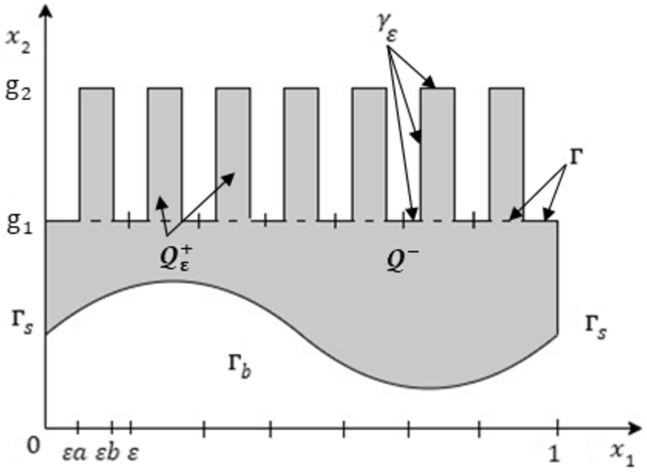We now present the detailed configuration of the oscillating domain ${\mathcal{Q}}_{\mathit{\epsilon }}$ . It is composed of two regions, the upper oscillating region ${\mathcal{Q}}_{\mathit{\epsilon }}^{+}$ , consisting of the slabs of height $\mathrm{(}{\mathit{g}}_2-{\mathit{g}}_1\mathrm{)}$ and width $\mathit{\epsilon }|\mathbb{A}|$ , and the bottom fixed region ${\mathcal{Q}}^{-}$ which is adjoint to ${\mathcal{Q}}_{\mathit{\epsilon }}^{+}$ at the interface ${\mathrm{\Gamma }}_{\mathit{\epsilon }}$ (see, Fig. 1). Mathematically, we can write $$\begin{array}{rl}& {\mathcal{Q}}_{\mathit{\epsilon }}=\{\mathrm{(}{\mathit{x}}_1\mathrm{,}{\mathit{x}}_2\mathrm{)}\in {\mathbb{R}}^2\mid {\mathit{x}}_1\in \mathrm{(}0\mathrm{,}1\mathrm{)}\mathrm{,}{\mathit{x}}_2\in \mathrm{(}\mathit{h}\mathrm{(}{\mathit{x}}_1\mathrm{)}\mathrm{,}{\mathit{\zeta }}_{\mathit{\epsilon }}\mathrm{(}{\mathit{x}}_1\mathrm{)}\mathrm{\left)}\right\}\mathrm{,}\\ & {\mathcal{Q}}_{\mathit{\epsilon }}^{+}={\displaystyle \bigcup }_{\mathit{n}=0}^{\mathit{k}-1}\{\mathrm{(}\mathit{n}\mathit{\epsilon }\mathrm{,}\mathit{n}\mathit{\epsilon }\mathrm{)}+\mathit{\epsilon }\mathbb{A}\}\times \mathrm{(}{\mathit{g}}_1\mathrm{,}{\mathit{g}}_2\mathrm{)}\mathrm{,}\\ & {\mathcal{Q}}^{-}=\{\mathrm{(}{\mathit{x}}_1\mathrm{,}{\mathit{x}}_2\mathrm{)}\in {\mathbb{R}}^2\mid {\mathit{x}}_1\in \mathrm{(}0\mathrm{,}1\mathrm{)}\mathrm{,}{\mathit{x}}_2\in \mathrm{(}\mathit{h}\mathrm{(}{\mathit{x}}_1\mathrm{)}\mathrm{,}{\mathit{g}}_1\mathrm{\left)}\right\}\mathrm{,}\\ & {\mathrm{\Gamma }}_{\mathit{\epsilon }}={\displaystyle \bigcup }_{\mathit{n}=0}^{\mathit{k}-1}\{\mathrm{(}\mathit{n}\mathit{\epsilon }\mathrm{,}\mathit{n}\mathit{\epsilon }\mathrm{)}+\mathit{\epsilon }\mathbb{A}\}\times \{{\mathit{g}}_1\}.\end{array}$$ The boundaries of ${\mathcal{Q}}_{\mathit{\epsilon }}$ viz., oscillating ${\mathit{\gamma }}_{\mathit{\epsilon }}$ , side ${\mathrm{\Gamma }}_{\mathit{s}}$ , and bottom ${\mathrm{\Gamma }}_{\mathit{b}}$ are defined as $$\begin{array}{rl}& {\mathrm{\Gamma }}_{\mathit{s}}=\{\mathrm{(}0\mathrm{,}{\mathit{x}}_2\mathrm{)}\mid {\mathit{x}}_2\in [\mathit{h}\mathrm{(}0\mathrm{)}\mathrm{,}{\mathit{g}}_1\left]\right\}\cup \{\mathrm{(}1\mathrm{,}{\mathit{x}}_2\mathrm{)}\mid {\mathit{x}}_2\in [\mathit{h}\mathrm{(}1\mathrm{)}\mathrm{,}{\mathit{g}}_1\left]\right\}\mathrm{,}\\ & {\mathrm{\Gamma }}_{\mathit{b}}=\left\{\mathrm{\right(}{\mathit{x}}_1\mathrm{,}\mathit{h}\mathrm{(}{\mathit{x}}_1\mathrm{)}\mathrm{)}\in {\mathbb{R}}^2\mid {\mathit{x}}_1\in [0\mathrm{,}1\mathrm{)}\}\mathrm{,}\\ & {\mathit{\gamma }}_{\mathit{\epsilon }}=\partial {\mathcal{Q}}_{\mathit{\epsilon }}\setminus \{{\mathrm{\Gamma }}_{\mathit{b}}\cup {\mathrm{\Gamma }}_{\mathit{s}}\}.\end{array}$$ The domain ${\mathcal{Q}}^{-}$ shares ${\mathrm{\Gamma }}_{\mathit{b}}$ and ${\mathrm{\Gamma }}_{\mathit{s}}$ as the common boundaries with ${\mathcal{Q}}_{\mathit{\epsilon }}$ . While we define its top boundary as $\mathrm{\Gamma }=\{\mathrm{(}{\mathit{x}}_1\mathrm{,}{\mathit{g}}_1\mathrm{)}\mid {\mathit{x}}_1\in [0\mathrm{,}1]\}$ .

Fig. 1.

The oscillating domain ${\mathcal{Q}}_{\mathit{\epsilon }}$ .

Fig. 2.

The fixed domain $\mathcal{Q}$ .

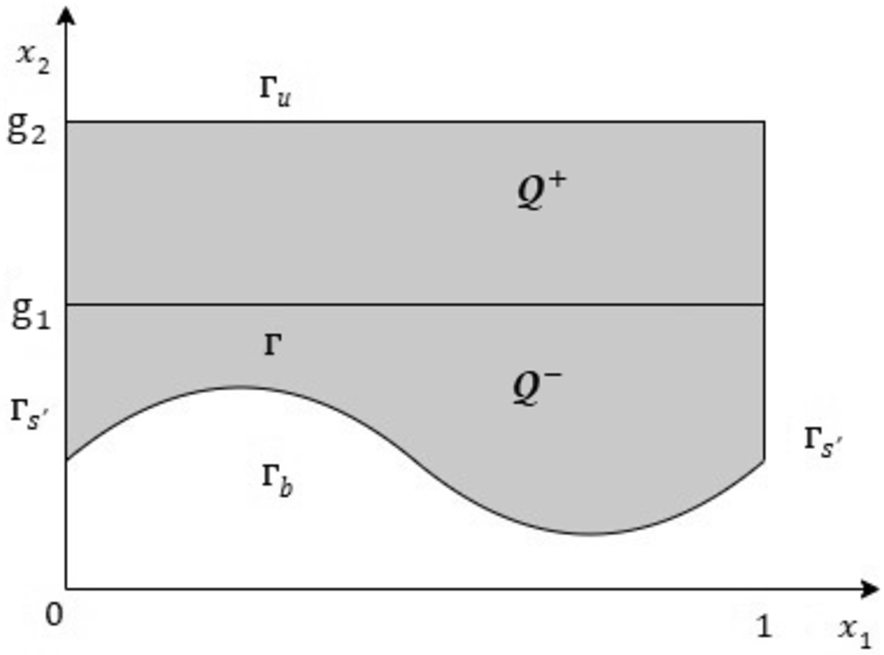
Next, we present the configuration of the limit domain $\mathcal{Q}$ . It is composed of two regions, the upper region ${\mathcal{Q}}^{+}$ , and the bottom region ${\mathcal{Q}}^{-}$ that are adjoined at the interface with Γ (see Fig. 2). Mathematically, we can write $$\begin{array}{c}\mathcal{Q}=\{\mathrm{(}{\mathit{x}}_1\mathrm{,}{\mathit{x}}_2\mathrm{)}\in {\mathbb{R}}^2\mid {\mathit{x}}_1\in \mathrm{(}0\mathrm{,}1\mathrm{)}\mathrm{,}\mathit{h}\mathrm{(}{\mathit{x}}_1\mathrm{)}\mathrm{<}{\mathit{x}}_2\mathrm{<}{\mathit{g}}_2\}.\end{array}$$ The bottom boundary ${\mathrm{\Gamma }}_{\mathit{b}}$ of $\mathcal{Q}$ is same as that of ${\mathcal{Q}}_{\mathit{\epsilon }}$ . The remaining boundaries viz., top ${\mathrm{\Gamma }}_{\mathit{u}}$ , and vertical ${\mathrm{\Gamma }}_{{\mathit{s}}^{\prime }}$ , are respectively defined as $$\begin{array}{rl}& {\mathrm{\Gamma }}_{\mathit{u}}=\{\mathrm{(}{\mathit{x}}_1\mathrm{,}{\mathit{g}}_2\mathrm{)}\mid {\mathit{x}}_1\in [0\mathrm{,}1]\}\mathrm{,}\\ & {\mathrm{\Gamma }}_{{\mathit{s}}^{\prime }}=\{\mathrm{(}0\mathrm{,}{\mathit{x}}_2\mathrm{)}\mid {\mathit{x}}_2\in [\mathit{h}\mathrm{(}0\mathrm{)}\mathrm{,}{\mathit{g}}_2\left]\right\}\cup \{\mathrm{(}1\mathrm{,}{\mathit{x}}_2\mathrm{)}\mid {\mathit{x}}_2\in [\mathit{h}\mathrm{(}1\mathrm{)}\mathrm{,}{\mathit{g}}_2\left]\right\}.\end{array}$$

2.2. Preliminaries

2.2.1. Notations

${\mathit{v}}_{\mathit{\epsilon }}=\mathrm{(}{\mathit{v}}_{\mathit{\epsilon }1}\mathrm{,}{\mathit{v}}_{\mathit{\epsilon }2}\mathrm{)}$ , for any bold symbol vector function ${\mathit{v}}_{\mathit{\epsilon }}$ .

$\mathit{v}=\mathrm{(}{\mathit{v}}_1\mathrm{,}{\mathit{v}}_2\mathrm{)}$ , for any bold symbol vector function $\mathit{v}$ .

$\mathit{\eta }\mathrm{>}0$ is a given regularization parameter.

${\mathit{u}}^{+}\mathrm{/}{\mathit{u}}^{+}$ denote the restriction of $\mathit{u}\mathrm{/}{\mathit{u}}^{+}$ on ${\mathcal{Q}}_{\mathit{\epsilon }}^{+}$ or ${\mathcal{Q}}^{+}$ .

${\mathit{u}}^{-}\mathrm{/}{\mathit{u}}^{+}$ denote the restriction of $\mathit{u}\mathrm{/}{\mathit{u}}^{+}$ on ${\mathcal{Q}}_{\mathit{\epsilon }}^{-}$ or ${\mathcal{Q}}^{-}$ .

$\mathit{u}{|}_{\mathit{D}}$ denotes the restriction of any function u over set D.

${\mathit{\mu }}_{\mathit{\epsilon }}$ denotes the outward normal unit vector to ${\mathit{\gamma }}_{\mathit{\epsilon }}$ .

$\mathit{K}\in {\mathbb{R}}^{+}$ is a generic constant that does not depend upon ε.

${\mathit{M}}^{\mathit{t}}$ denotes the transpose of any matrix M.

$\mathit{R}:\mathit{S}$ denotes the element-wise product followed by summation between any matrices R and S.

$\mathit{v}·\mathit{w}$ denotes the standard dot product between any vector functions $\mathit{v}$ and $\mathit{w}$ .

For $\mathit{i}\in \{1\mathrm{,}2\}$ , ${\partial }_{\mathit{i}}=\frac{\partial }{\partial {\mathit{x}}_{\mathit{i}}}$ and ${\partial }_{\mathit{y}}=\frac{\partial }{\partial \mathit{y}}$ .

$[\mathit{z}]$ and $\{\mathit{z}\}$ respectively denotes the greatest integer and the fractional parts of z, for all $\mathit{z}\in \mathbb{R}$ .

$\tilde{\mathit{\psi }}$ is the zero extension of any function ψ outside ${\mathcal{Q}}_{\mathit{\epsilon }}^{+}$ to the whole of ${\mathcal{Q}}_{\mathit{\epsilon }}$ .

$\tilde{\mathit{\psi }}=\mathrm{(}\widetilde{{\mathit{\psi }}_1}\mathrm{,}\widetilde{{\mathit{\psi }}_2}\mathrm{)}$ , for any vector function $\mathit{\psi }$ .

$|\mathit{F}|$ is the Lebesgue measure of the measurable set F.

The set $\{{\mathit{e}}_1\mathrm{,}{\mathit{e}}_2\}$ is the standard basis of ${\mathbb{R}}^2$ .

${\mathcal{M}}_{{\mathrm{(}0\mathrm{,}1\mathrm{)}}^2}\mathrm{(}\mathit{\varphi }\mathrm{)}$ is the mean value of ϕ on the reference cell ${\mathrm{(}0\mathrm{,}1\mathrm{)}}^2$ .

${\mathcal{M}}_{{\mathrm{(}0\mathrm{,}1\mathrm{)}}^2}\mathrm{(}\mathit{\varphi }\mathrm{)}=\mathrm{(}{\mathcal{M}}_{{\mathrm{(}0\mathrm{,}1\mathrm{)}}^2}\mathrm{(}{\mathit{\varphi }}_1\mathrm{)}\mathrm{,}{\mathcal{M}}_{{\mathrm{(}0\mathrm{,}1\mathrm{)}}^2}\mathrm{(}{\mathit{\varphi }}_2\mathrm{)}\mathrm{)}$ , for vector function $\mathit{\varphi }$ .

$\{\mathit{D}\to \mathbb{R}\}$ , the set of all real valued functions defined on domain D.

2.2.2. Function spaces and inequalities

Let us introduce the function spaces that will be used in the sequel:

${\mathrm{(}{\mathit{H}}_{\partial {\mathcal{Q}}_{\mathit{\epsilon }}\setminus {\mathit{\gamma }}_{\mathit{\epsilon }}}^1\mathrm{(}{\mathcal{Q}}_{\mathit{\epsilon }}\mathrm{)}\mathrm{)}}^2:=\{\mathit{v}\in {\mathrm{(}{\mathit{H}}^1\mathrm{(}{\mathcal{Q}}_{\mathit{\epsilon }}\mathrm{)}\mathrm{)}}^2\mid \mathit{v}{|}_{\partial {\mathcal{Q}}_{\mathit{\epsilon }}\setminus {\mathit{\gamma }}_{\mathit{\epsilon }}}=0\}$ .

${\mathrm{(}{\mathit{U}}_{\partial \mathcal{Q}\setminus {\mathrm{\Gamma }}_{\mathit{u}}}\mathrm{(}\mathcal{Q}\mathrm{)}\mathrm{)}}^2:=\{\mathit{\varphi }\in {\mathrm{(}{\mathit{L}}^2\mathrm{(}\mathcal{Q}\mathrm{)}\mathrm{)}}^2:{\mathit{\varphi }}^{\mathbf{-}}\in {\mathrm{(}{\mathit{H}}^1\mathrm{(}{\mathcal{Q}}^{-}\mathrm{)}\mathrm{)}}^2\mathrm{,}{\partial }_2{\mathit{\varphi }}^{+}\in {\mathrm{(}{\mathit{L}}^2\mathrm{(}{\mathcal{Q}}^{+}\mathrm{)}\mathrm{)}}^2\text{ and }\mathit{\varphi }{|}_{\partial \mathcal{Q}\setminus {\mathrm{\Gamma }}_{\mathit{u}}}=0\}$ .

${\mathrm{(}{\mathit{U}}_{\mathit{\sigma }\mathrm{,}\partial \mathcal{Q}\setminus {\mathrm{\Gamma }}_{\mathit{u}}}\mathrm{(}\mathcal{Q}\mathrm{)}\mathrm{)}}^2:=\{\mathit{\varphi }\in {\mathrm{(}{\mathit{U}}_{\partial \mathcal{Q}\setminus {\mathrm{\Gamma }}_{\mathit{u}}}\mathrm{(}\mathcal{Q}\mathrm{)}\mathrm{)}}^2:div\mathrm{(}{\mathbf{\Phi }}^{\mathbf{-}}\mathrm{)}=0\text{ on }{\mathcal{Q}}^{-}\}$ . This is a Hilbert space with respect to the norm $$\begin{array}{c}\Vert {\mathit{\varphi }\Vert }_{{\mathrm{(}{\mathit{U}}_{\partial \mathcal{Q}\setminus {\mathrm{\Gamma }}_{\mathit{u}}}\mathrm{(}\mathcal{Q}\mathrm{)}\mathrm{)}}^2}^2={\Vert {\mathit{\varphi }}^{\mathbf{-}}\Vert }_{{\mathrm{(}{\mathit{H}}^1\mathrm{(}{\mathcal{Q}}^{-}\mathrm{)}\mathrm{)}}^2}^2+{\Vert {\mathit{\varphi }}^{\mathbf{+}}\Vert }_{{\mathrm{(}{\mathit{L}}^2\mathrm{(}{\mathcal{Q}}^{+}\mathrm{)}\mathrm{)}}^2}^2+{\Vert {\partial }_2{\mathit{\varphi }}^{+}\Vert }_{{\mathrm{(}{\mathit{L}}^2\mathrm{(}{\mathcal{Q}}^{+}\mathrm{)}\mathrm{)}}^2}^2.\end{array}$$ The space ${\mathrm{(}{\mathit{U}}_{\mathit{\sigma }\mathrm{,}\partial \mathcal{Q}\setminus {\mathrm{\Gamma }}_{\mathit{u}}}\mathrm{(}\mathcal{Q}\mathrm{)}\mathrm{)}}^2$ is a closed in ${\mathrm{(}{\mathit{U}}_{\partial \mathcal{Q}\setminus {\mathrm{\Gamma }}_{\mathit{u}}}\mathrm{(}\mathcal{Q}\mathrm{)}\mathrm{)}}^2$ with respect to the norm endowed on the latter. We define ${\mathrm{(}{\mathit{C}}_{\partial \mathcal{Q}\setminus {\mathrm{\Gamma }}_{\mathit{u}}}^{\infty }\mathrm{(}\bar{\mathcal{Q}}\mathrm{)}\mathrm{)}}^2:=\{\mathit{\varphi }\in {\mathrm{(}{\mathit{C}}^{\infty }\mathrm{(}\bar{\mathcal{Q}}\mathrm{)}\mathrm{)}}^2:\mathit{\varphi }{|}_{\partial \mathcal{Q}\setminus {\mathrm{\Gamma }}_{\mathit{u}}}=0\}$ , which is a dense subspace of ${\mathrm{(}{\mathit{U}}_{\partial \mathcal{Q}\setminus {\mathrm{\Gamma }}_{\mathit{u}}}\mathrm{(}\mathcal{Q}\mathrm{)}\mathrm{)}}^2$ , with respect to the norm in ${\mathrm{(}{\mathit{U}}_{\partial \mathcal{Q}\setminus {\mathrm{\Gamma }}_{\mathit{u}}}\mathrm{(}\mathcal{Q}\mathrm{)}\mathrm{)}}^2$ (see [11, Proposition 4.1]).

Next, we will repeatedly make use of the following inequalities. Throughout this article, $\mathit{K}\in {\mathbb{R}}^{+}$ is a generic constant that does not depend upon ε.

• Poincaré inequality, [24, Lemma 2.2]: For each $\mathit{\epsilon }\mathrm{>}0$ , there exists $\mathit{K}\in {\mathbb{R}}^{+}$ , such that $$\begin{array}{}\text{(2.1)}& \Vert \mathit{g}{\Vert }_{{\mathit{L}}^2\mathrm{(}{\mathcal{Q}}_{\mathit{\epsilon }}\mathrm{)}}⩽\mathit{K}\Vert \nabla \mathit{g}{\Vert }_{{\mathrm{(}{\mathit{L}}^2\mathrm{(}{\mathcal{Q}}_{\mathit{\epsilon }}\mathrm{)}\mathrm{)}}^2}\mathrm{,}\forall \mathit{g}\in {\mathit{H}}_{{\mathit{\gamma }}_{\mathit{l}}}^1\mathrm{(}{\mathcal{Q}}_{\mathit{\epsilon }}\mathrm{)}.\end{array}$$

• Bogovski operator theorem, [24, Lemma 2.3]: For each $\mathit{\epsilon }\mathrm{>}0$ and ${\mathit{q}}_{\mathit{\epsilon }}\in {\mathit{L}}^2\mathrm{(}{\mathcal{Q}}_{\mathit{\epsilon }}\mathrm{)}$ , there exists a ${\mathit{g}}_{\mathit{\epsilon }}\in {\mathrm{(}{\mathit{H}}_{\partial {\mathcal{Q}}_{\mathit{\epsilon }}\setminus {\mathit{\gamma }}_{\mathit{\epsilon }}}^1\mathrm{(}{\mathcal{Q}}_{\mathit{\epsilon }}\mathrm{)}\mathrm{)}}^2$ and $\mathit{K}\in {\mathbb{R}}^{+}$ , such that $$\begin{array}{}\text{(2.2)}& div\mathrm{(}{\mathit{g}}_{\mathit{\epsilon }}\mathrm{)}={\mathit{q}}_{\mathit{\epsilon }}\text{and}\Vert \nabla {\mathit{g}}_{\mathit{\epsilon }}{\Vert }_{{\mathrm{(}{\mathit{L}}^2\mathrm{(}{\mathcal{Q}}_{\mathit{\epsilon }}\mathrm{)}\mathrm{)}}^{2\times 2}}⩽\mathit{K}\mathrm{(}\mathcal{Q}\mathrm{)}\Vert {\mathit{q}}_{\mathit{\epsilon }}{\Vert }_{{\mathit{L}}^2\mathrm{(}{\mathcal{Q}}_{\mathit{\epsilon }}\mathrm{)}}.\end{array}$$

Let us impose the following assumptions on the matrices ${\mathit{A}}_{\mathit{\epsilon }}={\mathrm{(}{\mathit{a}}_{\mathit{i}\mathit{j}}\mathrm{(}\mathit{x}\mathrm{,}\frac{{\mathit{x}}_1}{\mathit{\epsilon }}\mathrm{)}\mathrm{)}}_{1⩽\mathit{i}\mathrm{,}\mathit{j}⩽2}$ and ${\mathit{B}}_{\mathit{\epsilon }}={\mathrm{(}{\mathit{b}}_{\mathit{i}\mathit{j}}\mathrm{(}\mathit{x}\mathrm{,}\frac{{\mathit{x}}_1}{\mathit{\epsilon }}\mathrm{)}\mathrm{)}}_{1⩽\mathit{i}\mathrm{,}\mathit{j}⩽2}$ considered in the OCP (1.2):

• ${\mathit{A}}_{\mathit{\epsilon }}$ is elliptic. That is, there exist real constants ${\mathit{\alpha }}_1\mathrm{,}{\mathit{\alpha }}_2\mathrm{>}0$ , such that: $$\begin{array}{c}{\mathit{\alpha }}_1\Vert \mathit{\lambda }{\Vert }^2⩽{\displaystyle \sum }_{\mathit{i}\mathrm{,}\mathit{j}=1}^2{\mathit{a}}_{\mathit{i}\mathit{j}}\mathrm{(}\mathit{x}\mathrm{,}{\displaystyle \frac{{\mathit{x}}_1}{\mathit{\epsilon }}}\mathrm{)}{\mathit{\lambda }}_{\mathit{i}}{\mathit{\lambda }}_{\mathit{j}}⩽{\mathit{\alpha }}_2\Vert \mathit{\lambda }{\Vert }^2\text{for all }\mathit{\lambda }\in {\mathbb{R}}^2\text{ and a.e. on }{\mathbb{R}}^2.\end{array}$$

• ${\mathit{B}}_{\mathit{\epsilon }}$ is symmetric and elliptic. By latter, we mean that there exist real constants ${\mathit{\beta }}_1\mathrm{,}{\mathit{\beta }}_2\mathrm{>}0$ such that: $$\begin{array}{c}{\mathit{\beta }}_1\Vert \mathit{\lambda }{\Vert }^2⩽{\displaystyle \sum }_{\mathit{i}\mathrm{,}\mathit{j}=1}^2{\mathit{b}}_{\mathit{i}\mathit{j}}\mathrm{(}\mathit{x}\mathrm{,}{\displaystyle \frac{{\mathit{x}}_1}{\mathit{\epsilon }}}\mathrm{)}{\mathit{\lambda }}_{\mathit{i}}{\mathit{\lambda }}_{\mathit{j}}⩽{\mathit{\beta }}_2\Vert \mathit{\lambda }{\Vert }^2\text{for all }\mathit{\lambda }\in {\mathbb{R}}^2\text{ and a.e. on }{\mathbb{R}}^2.\end{array}$$

3. Optimality condition and norm-estimates

3.1. Optimality condition

Here, we present the characterization result for the optimal control, which minimizes the OCP (1.2). Let us first write the weak formulation of the problem (1.1).

Definition 3.1.

We call a pair $\mathrm{(}{\mathit{u}}_{\mathit{\epsilon }}\mathrm{,}{\mathit{p}}_{\mathit{\epsilon }}\mathrm{)}\in {\mathrm{(}{\mathit{H}}_{\partial {\mathcal{Q}}_{\mathit{\epsilon }}\setminus {\mathit{\gamma }}_{\mathit{\epsilon }}}^1\mathrm{(}{\mathcal{Q}}_{\mathit{\epsilon }}\mathrm{)}\mathrm{)}}^2\times {\mathit{L}}^2\mathrm{(}{\mathcal{Q}}_{\mathit{\epsilon }}\mathrm{)}$ to be a weak solution to (1.1) if, for all $\mathit{v}\in {\mathrm{(}{\mathit{H}}_{\partial {\mathcal{Q}}_{\mathit{\epsilon }}\setminus {\mathit{\gamma }}_{\mathit{\epsilon }}}^1\mathrm{(}{\mathcal{Q}}_{\mathit{\epsilon }}\mathrm{)}\mathrm{)}}^2$ , $$\begin{array}{}\text{(3.1)}& {{\displaystyle \int }}_{{\mathcal{Q}}_{\mathit{\epsilon }}}{\mathit{A}}_{\mathit{\epsilon }}\nabla {\mathit{u}}_{\mathit{\epsilon }}:\nabla \mathit{v}\mathit{d}\mathit{x}-{{\displaystyle \int }}_{{\mathcal{Q}}_{\mathit{\epsilon }}}{\mathit{p}}_{\mathit{\epsilon }}div\mathrm{(}\mathit{v}\mathrm{)}\mathit{d}\mathit{x}={{\displaystyle \int }}_{{\mathcal{Q}}_{\mathit{\epsilon }}}\mathrm{(}\mathit{f}+{\mathit{\theta }}_{\mathit{\epsilon }}\mathrm{)}·\mathit{v}\mathit{d}\mathit{x}\mathrm{,}\end{array}$$ and, for all $\mathit{w}\in {\mathit{L}}^2\mathrm{(}{\mathcal{Q}}_{\mathit{\epsilon }}\mathrm{)}$ , $$\begin{array}{}\text{(3.2)}& {{\displaystyle \int }}_{{\mathcal{Q}}_{\mathit{\epsilon }}}div\mathrm{(}{\mathit{u}}_{\mathit{\epsilon }}\mathrm{)}\mathit{w}\mathit{d}\mathit{x}=0.\end{array}$$

As mentioned in the Introduction, for each $\mathit{\epsilon }\mathrm{>}0$ , the problem (1.1) admits a unique weak solution $\mathrm{(}{\mathit{u}}_{\mathit{\epsilon }}\mathrm{(}{\mathit{\theta }}_{\mathit{\epsilon }}\mathrm{)}\mathrm{,}{\mathit{p}}_{\mathit{\epsilon }}\mathrm{)}\in {\mathrm{(}{\mathit{H}}_{\partial {\mathcal{Q}}_{\mathit{\epsilon }}\setminus {\mathit{\gamma }}_{\mathit{\epsilon }}}^1\mathrm{(}{\mathcal{Q}}_{\mathit{\epsilon }}\mathrm{)}\mathrm{)}}^2\times {\mathit{L}}^2\mathrm{(}{\mathcal{Q}}_{\mathit{\epsilon }}\mathrm{)}$ , the proof of which is standard one and follows quickly along the lines of [17, Remark 2.1] by employing the ellipticity of matrix ${\mathit{A}}_{\mathit{\epsilon }}$ . Moreover, a unique minimizer to the OCP (1.2) exists. Let us denote it by ${\bar{\mathit{\theta }}}_{\mathit{\epsilon }}\in {\mathrm{(}{\mathit{L}}^2\mathrm{(}{\mathcal{Q}}_{\mathit{\epsilon }}\mathrm{)}\mathrm{)}}^2$ and the associated solution to (1.1) by $\mathrm{(}{\bar{\mathit{u}}}_{\mathit{\epsilon }}\mathrm{,}{\bar{\mathit{p}}}_{\mathit{\epsilon }}\mathrm{)}\in {\mathrm{(}{\mathit{H}}_{\partial {\mathcal{Q}}_{\mathit{\epsilon }}\setminus {\mathit{\gamma }}_{\mathit{\epsilon }}}^1\mathrm{(}{\mathcal{Q}}_{\mathit{\epsilon }}\mathrm{)}\mathrm{)}}^2\times {\mathit{L}}^2\mathrm{(}{\mathcal{Q}}_{\mathit{\epsilon }}\mathrm{)}$ , where the terms ${\bar{\mathit{\theta }}}_{\mathit{\epsilon }}$ , ${\bar{\mathit{u}}}_{\mathit{\epsilon }}$ , and ${\bar{\mathit{p}}}_{\mathit{\epsilon }}$ are respectively the optimal control, state, and pressure. We denote the optimal solution to the OCP (1.2) by a triplet $\mathrm{(}{\bar{\mathit{u}}}_{\mathit{\epsilon }}\mathrm{,}{\bar{\mathit{p}}}_{\mathit{\epsilon }}\mathrm{,}{\bar{\mathit{\theta }}}_{\mathit{\epsilon }}\mathrm{)}$ .

Next, let us consider the associated adjoint problem to (1.1): Find $\mathrm{(}{\bar{\mathit{v}}}_{\mathit{\epsilon }}\mathrm{,}{\bar{\mathit{q}}}_{\mathit{\epsilon }}\mathrm{)}\in {\mathrm{(}{\mathit{H}}_{\partial {\mathcal{Q}}_{\mathit{\epsilon }}\setminus {\mathit{\gamma }}_{\mathit{\epsilon }}}^1\mathrm{(}{\mathcal{Q}}_{\mathit{\epsilon }}\mathrm{)}\mathrm{)}}^2\times {\mathit{L}}^2\mathrm{(}{\mathcal{Q}}_{\mathit{\epsilon }}\mathrm{)}$ that obeys the following system: $$\begin{array}{}\text{(3.3)}& \left\{\begin{array}{ll}-div\mathrm{(}{\mathit{A}}_{\mathit{\epsilon }}^{\mathit{t}}\nabla {\bar{\mathit{v}}}_{\mathit{\epsilon }}\mathrm{)}+\nabla {\bar{\mathit{q}}}_{\mathit{\epsilon }}=-div\mathrm{(}{\mathit{B}}_{\mathit{\epsilon }}\nabla {\bar{\mathit{u}}}_{\mathit{\epsilon }}\mathrm{)}& \text{in }{\mathcal{Q}}_{\mathit{\epsilon }}\mathrm{,}\\ div\mathrm{(}{\bar{\mathit{v}}}_{\mathit{\epsilon }}\mathrm{)}=0& \text{in }{\mathcal{Q}}_{\mathit{\epsilon }}\mathrm{,}\\ {\mathit{\mu }}_{\mathit{\epsilon }}·{\mathit{A}}_{\mathit{\epsilon }}^{\mathit{t}}\nabla {\bar{\mathit{v}}}_{\mathit{\epsilon }}-{\bar{\mathit{q}}}_{\mathit{\epsilon }}{\mathit{\mu }}_{\mathit{\epsilon }}={\mathit{\mu }}_{\mathit{\epsilon }}·{\mathit{B}}_{\mathit{\epsilon }}\nabla {\bar{\mathit{u}}}_{\mathit{\epsilon }}& \text{on }{\mathit{\gamma }}_{\mathit{\epsilon }}\mathrm{,}\\ {\bar{\mathit{v}}}_{\mathit{\epsilon }}=\mathbf{0}& \text{on }\partial {\mathcal{Q}}_{\mathit{\epsilon }}\setminus {\mathit{\gamma }}_{\mathit{\epsilon }}.\end{array}\right.\end{array}$$ A unique weak solution $\mathrm{(}{\bar{\mathit{v}}}_{\mathit{\epsilon }}\mathrm{,}{\bar{\mathit{q}}}_{\mathit{\epsilon }}\mathrm{)}\in {\mathrm{(}{\mathit{H}}_{\partial {\mathcal{Q}}_{\mathit{\epsilon }}\setminus {\mathit{\gamma }}_{\mathit{\epsilon }}}^1\mathrm{(}{\mathcal{Q}}_{\mathit{\epsilon }}\mathrm{)}\mathrm{)}}^2\times {\mathit{L}}^2\mathrm{(}{\mathcal{Q}}_{\mathit{\epsilon }}\mathrm{)}$ to the adjoint problem (3.3) exists, which is easy to establish analogous to the state equation (1.1) by using the ellipticity of the matrices ${\mathit{A}}_{\mathit{\epsilon }}^{\mathit{t}}$ and ${\mathit{B}}_{\mathit{\epsilon }}$ . We denote the terms ${\bar{\mathit{v}}}_{\mathit{\epsilon }}$ , and ${\bar{\mathit{q}}}_{\mathit{\epsilon }}$ respectively by the adjoint state and pressure. In the below-mentioned result, we characterize the optimal control in terms of the adjoint state solving the adjoint system (3.3). The proof of which is a standard argument and follows analogous to [30, Theorem 2.7.1]. Theorem 3.2.

Let $\mathrm{(}{\bar{\mathit{u}}}_{\mathit{\epsilon }}\mathrm{,}{\bar{\mathit{p}}}_{\mathit{\epsilon }}\mathrm{,}{\bar{\mathit{\theta }}}_{\mathit{\epsilon }}\mathrm{)}$ be the optimal solution of the problem ( 1.2 ) and the pair $\mathrm{(}{\bar{\mathit{v}}}_{\mathit{\epsilon }}\mathrm{,}{\bar{\mathit{q}}}_{\mathit{\epsilon }}\mathrm{)}$ satisfies ( 3.3 ), then the optimal control ${\bar{\mathit{\theta }}}_{\mathit{\epsilon }}\in {\mathrm{(}{\mathit{L}}^2\mathrm{(}{\mathcal{Q}}_{\mathit{\epsilon }}\mathrm{)}\mathrm{)}}^2$ is given by $$\begin{array}{}\text{(3.4)}& {\bar{\mathit{\theta }}}_{\mathit{\epsilon }}\mathrm{(}\mathit{x}\mathrm{)}=-{\displaystyle \frac{1}{\mathit{\eta }}}{\bar{\mathit{v}}}_{\mathit{\epsilon }}\mathrm{(}\mathit{x}\mathrm{)}\mathit{\text{a.e. in }}{\mathcal{Q}}_{\mathit{\epsilon }}.\end{array}$$ Conversely, assume that a triplet $\mathrm{(}{\check{\mathit{u}}}_{\mathit{\epsilon }}\mathrm{,}{\check{\mathit{p}}}_{\mathit{\epsilon }}\mathrm{,}-\frac{1}{\mathit{\eta }}{\check{\mathit{v}}}_{\mathit{\epsilon }}\mathrm{)}\in {\mathrm{(}{\mathit{H}}_{\partial {\mathcal{Q}}_{\mathit{\epsilon }}\setminus {\mathit{\gamma }}_{\mathit{\epsilon }}}^1\mathrm{(}{\mathcal{Q}}_{\mathit{\epsilon }}\mathrm{)}\mathrm{)}}^2\times {\mathit{L}}^2\mathrm{(}{\mathcal{Q}}_{\mathit{\epsilon }}\mathrm{)}\times {\mathrm{(}{\mathit{L}}^2\mathrm{(}{\mathcal{Q}}_{\mathit{\epsilon }}\mathrm{)}\mathrm{)}}^2$ and a pair $\mathrm{(}{\check{\mathit{v}}}_{\mathit{\epsilon }}\mathrm{,}{\check{\mathit{q}}}_{\mathit{\epsilon }}\mathrm{)}\in {\mathrm{(}{\mathit{H}}_{\partial {\mathcal{Q}}_{\mathit{\epsilon }}\setminus {\mathit{\gamma }}_{\mathit{\epsilon }}}^1\mathrm{(}{\mathcal{Q}}_{\mathit{\epsilon }}\mathrm{)}\mathrm{)}}^2\times {\mathit{L}}^2\mathrm{(}{\mathcal{Q}}_{\mathit{\epsilon }}\mathrm{)}$ satisfy the following system $$\begin{array}{}\text{(3.5)}& \left\{\begin{array}{ll}-div\mathrm{(}{\mathit{A}}_{\mathit{\epsilon }}\nabla {\check{\mathit{u}}}_{\mathit{\epsilon }}\mathrm{)}+\nabla {\check{\mathit{p}}}_{\mathit{\epsilon }}=\mathit{f}-\frac{1}{\mathit{\eta }}{\check{\mathit{v}}}_{\mathit{\epsilon }}& \mathit{\text{in }}{\mathcal{Q}}_{\mathit{\epsilon }}\mathrm{,}\\ -div\mathrm{(}{\mathit{A}}_{\mathit{\epsilon }}^{\mathit{t}}\nabla {\check{\mathit{v}}}_{\mathit{\epsilon }}\mathrm{)}+\nabla {\check{\mathit{q}}}_{\mathit{\epsilon }}=-div\mathrm{(}{\mathit{B}}_{\mathit{\epsilon }}\nabla {\check{\mathit{u}}}_{\mathit{\epsilon }}\mathrm{)}& \mathit{\text{in }}{\mathcal{Q}}_{\mathit{\epsilon }}\mathrm{,}\\ div\mathrm{(}{\check{\mathit{u}}}_{\mathit{\epsilon }}\mathrm{)}=0\mathrm{,}div\mathrm{(}{\check{\mathit{v}}}_{\mathit{\epsilon }}\mathrm{)}=0& \mathit{\text{in }}{\mathcal{Q}}_{\mathit{\epsilon }}\mathrm{,}\\ {\mathit{\mu }}_{\mathit{\epsilon }}·{\mathit{A}}_{\mathit{\epsilon }}\nabla {\check{\mathit{u}}}_{\mathit{\epsilon }}-{\check{\mathit{p}}}_{\mathit{\epsilon }}{\mathit{\mu }}_{\mathit{\epsilon }}=\mathbf{0}& \mathit{\text{on }}{\mathit{\gamma }}_{\mathit{\epsilon }}\mathrm{,}\\ {\mathit{\mu }}_{\mathit{\epsilon }}·{\mathit{A}}_{\mathit{\epsilon }}^{\mathit{t}}\nabla {\check{\mathit{v}}}_{\mathit{\epsilon }}-{\bar{\mathit{q}}}_{\mathit{\epsilon }}{\mathit{\mu }}_{\mathit{\epsilon }}={\mathit{\mu }}_{\mathit{\epsilon }}·{\mathit{B}}_{\mathit{\epsilon }}\nabla {\check{\mathit{u}}}_{\mathit{\epsilon }}& \mathit{\text{on }}{\mathit{\gamma }}_{\mathit{\epsilon }}\mathrm{,}\\ {\check{\mathit{v}}}_{\mathit{\epsilon }}=\mathbf{0}\mathrm{,}{\check{\mathit{u}}}_{\mathit{\epsilon }}=\mathbf{0}& \mathit{\text{on }}\partial {\mathcal{Q}}_{\mathit{\epsilon }}\setminus {\mathit{\gamma }}_{\mathit{\epsilon }}.\end{array}\right.\end{array}$$ Then the triplet $\mathrm{(}{\check{\mathit{u}}}_{\mathit{\epsilon }}\mathrm{,}{\check{\mathit{p}}}_{\mathit{\epsilon }}\mathrm{,}-\frac{1}{\mathit{\eta }}{\check{\mathit{v}}}_{\mathit{\epsilon }}\mathrm{)}$ is the optimal solution to ( 1.2 ).

3.2. Norm-estimates

We now derive the norm-estimates, uniform in ε, for the triplet $\mathrm{(}{\bar{\mathit{u}}}_{\mathit{\epsilon }}\mathrm{,}{\bar{\mathit{p}}}_{\mathit{\epsilon }}\mathrm{,}{\bar{\mathit{\theta }}}_{\mathit{\epsilon }}\mathrm{)}$ solving the OCP (1.2) and the pair $\mathrm{(}{\bar{\mathit{v}}}_{\mathit{\epsilon }}\mathrm{,}{\bar{\mathit{q}}}_{\mathit{\epsilon }}\mathrm{)}$ the solving (3.3).

Theorem 3.3.

For given $\mathit{\epsilon }\mathrm{>}0$ , let the optimal control to ( 1.2 ) be ${\bar{\mathit{\theta }}}_{\mathit{\epsilon }}\in {\mathrm{(}{\mathit{L}}^2\mathrm{(}{\mathcal{Q}}_{\mathit{\epsilon }}\mathrm{)}\mathrm{)}}^2$ . Then the following sequences are bounded uniformly in ε: $$\begin{array}{}\text{(3.6)}& & \Vert {\bar{\mathit{\theta }}}_{\mathit{\epsilon }}{\Vert }_{{\mathrm{(}{\mathit{L}}^2\mathrm{(}{\mathcal{Q}}_{\mathit{\epsilon }}\mathrm{)}\mathrm{)}}^2}⩽\mathit{K}\mathrm{,}\text{(3.7)}& & \Vert {\bar{\mathit{u}}}_{\mathit{\epsilon }}{\Vert }_{{\mathrm{(}{\mathit{H}}_{\partial {\mathcal{Q}}_{\mathit{\epsilon }}\setminus {\mathit{\gamma }}_{\mathit{\epsilon }}}^1\mathrm{(}{\mathcal{Q}}_{\mathit{\epsilon }}\mathrm{)}\mathrm{)}}^2}⩽\mathit{K}\mathrm{,}\text{(3.8)}& & \Vert {\bar{\mathit{p}}}_{\mathit{\epsilon }}{\Vert }_{{\mathit{L}}^2\mathrm{(}{\mathcal{Q}}_{\mathit{\epsilon }}\mathrm{)}}⩽\mathit{K}\mathrm{,}\text{(3.9)}& & \Vert {\bar{\mathit{v}}}_{\mathit{\epsilon }}{\Vert }_{{\mathrm{(}{\mathit{H}}_{\partial {\mathcal{Q}}_{\mathit{\epsilon }}\setminus {\mathit{\gamma }}_{\mathit{\epsilon }}}^1\mathrm{(}{\mathcal{Q}}_{\mathit{\epsilon }}\mathrm{)}\mathrm{)}}^2}⩽\mathit{K}\mathrm{,}\text{(3.10)}& & \Vert {\bar{\mathit{q}}}_{\mathit{\epsilon }}{\Vert }_{{\mathit{L}}^2\mathrm{(}{\mathcal{Q}}_{\mathit{\epsilon }}\mathrm{)}}⩽\mathit{K}.\end{array}$$

Proof.

Taking zero control in (1.1), we denote the corresponding state function by ${\mathit{u}}_{\mathit{\epsilon }}\mathrm{(}\mathbf{0}\mathrm{)}$ . Taking into account the ellipticity of matrix ${\mathit{B}}_{\mathit{\epsilon }}$ and the optimality condition for the cost functional, i.e., ${\mathit{J}}_{\mathit{\epsilon }}\mathrm{(}{\bar{\mathit{\theta }}}_{\mathit{\epsilon }}\mathrm{)}⩽\mathit{J}\mathrm{(}\mathbf{0}\mathrm{)}$ , we get $$\begin{array}{c}{\mathit{\alpha }}_2{\Vert \nabla {\bar{\mathit{u}}}_{\mathit{\epsilon }}\mathrm{(}\bar{\mathit{\theta }}\mathrm{)}\Vert }_{{\mathrm{(}{\mathit{L}}^2\mathrm{(}{\mathcal{Q}}_{\mathit{\epsilon }}\mathrm{)}\mathrm{)}}^{2\times 2}}^2+\mathit{\eta }\Vert {\bar{\mathit{\theta }}}_{\mathit{\epsilon }}{\Vert }_{{\mathrm{(}{\mathit{L}}^2\mathrm{(}{\mathcal{Q}}_{\mathit{\epsilon }}\mathrm{)}\mathrm{)}}^2}^2⩽{\mathit{\beta }}_2{\Vert \nabla {\mathit{u}}_{\mathit{\epsilon }}\mathrm{(}\mathbf{0}\mathrm{)}\Vert }_{{\mathrm{(}{\mathit{L}}^2\mathrm{(}{\mathcal{Q}}_{\mathit{\epsilon }}\mathrm{)}\mathrm{)}}^{2\times 2}}^2\mathrm{,}\end{array}$$ which implies that $$\begin{array}{}\text{(3.11)}& \Vert {\bar{\mathit{\theta }}}_{\mathit{\epsilon }}{\Vert }_{{\mathrm{(}{\mathit{L}}^2\mathrm{(}{\mathcal{Q}}_{\mathit{\epsilon }}\mathrm{)}\mathrm{)}}^2}⩽{\displaystyle \frac{\sqrt{{\mathit{\beta }}_2}}{\sqrt{\mathit{\eta }}}}{\Vert \nabla {\mathit{u}}_{\mathit{\epsilon }}\mathrm{(}\mathbf{0}\mathrm{)}\Vert }_{{\mathrm{(}{\mathit{L}}^2\mathrm{(}{\mathcal{Q}}_{\mathit{\epsilon }}\mathrm{)}\mathrm{)}}^{2\times 2}}.\end{array}$$ In order to obtain the first estimate (3.6), we need to further simplify the right-hand side of (3.11). To do so, we plug in the data $\mathit{v}={\mathit{u}}_{\mathit{\epsilon }}$ and $\mathit{w}={\mathit{p}}_{\mathit{\epsilon }}$ in (3.1) and (3.2), respectively. Taking into account the ellipticity of matrix ${\mathit{A}}_{\mathit{\epsilon }}$ and (2.1), we obtain $$\begin{array}{c}{\mathit{\alpha }}_1\Vert \nabla {\mathit{u}}_{\mathit{\epsilon }}{\Vert }_{{\mathrm{(}{\mathit{L}}^2\mathrm{(}{\mathcal{Q}}_{\mathit{\epsilon }}\mathrm{)}\mathrm{)}}^{2\times 2}}^2⩽{{\displaystyle \int }}_{{\mathcal{Q}}_{\mathit{\epsilon }}}{\mathit{A}}_{\mathit{\epsilon }}\mathrm{(}\mathit{x}\mathrm{)}\nabla {\mathit{u}}_{\mathit{\epsilon }}:\nabla {\mathit{u}}_{\mathit{\epsilon }}\mathit{d}\mathit{x}⩽\mathrm{(}\Vert \mathit{f}{\Vert }_{{\mathrm{(}{\mathit{L}}^2\mathrm{(}\mathcal{Q}\mathrm{)}\mathrm{)}}^2}+{\mathit{\beta }}_1\Vert {\mathit{\theta }}_{\mathit{\epsilon }}{\Vert }_{{\mathrm{(}{\mathit{L}}^2\mathrm{(}{\mathcal{Q}}_{\mathit{\epsilon }}\mathrm{)}\mathrm{)}}^2}\mathrm{)}\Vert \nabla {\mathit{u}}_{\mathit{\epsilon }}{\Vert }_{{\mathrm{(}{\mathit{L}}^2\mathrm{(}{\mathcal{Q}}_{\mathit{\epsilon }}\mathrm{)}\mathrm{)}}^{2\times 2}}\mathrm{,}\end{array}$$ which upon further simplification, gives $$\begin{array}{}\text{(3.12)}& \Vert \nabla {\mathit{u}}_{\mathit{\epsilon }}{\Vert }_{{\mathrm{(}{\mathit{L}}^2\mathrm{(}{\mathcal{Q}}_{\mathit{\epsilon }}\mathrm{)}\mathrm{)}}^{2\times 2}}⩽\mathit{K}\mathrm{(}\Vert \mathit{f}{\Vert }_{{\mathrm{(}{\mathit{L}}^2\mathrm{(}\mathcal{Q}\mathrm{)}\mathrm{)}}^2}+\Vert {\mathit{\theta }}_{\mathit{\epsilon }}{\Vert }_{{\mathrm{(}{\mathit{L}}^2\mathrm{(}{\mathcal{Q}}_{\mathit{\epsilon }}\mathrm{)}\mathrm{)}}^2}\mathrm{)}.\end{array}$$ From (3.12) corresponding to $\mathit{\theta }=\mathbf{0}$ , we have $\Vert \nabla {\mathit{u}}_{\mathit{\epsilon }}\mathrm{(}\mathbf{0}\mathrm{)}{\Vert }_{{\mathrm{(}{\mathit{L}}^2\mathrm{(}{\mathcal{Q}}_{\mathit{\epsilon }}\mathrm{)}\mathrm{)}}^{2\times 2}}⩽\mathit{K}$ . Employing this together with (2.1) in (3.11) establishes (3.6). Again, from (3.12), we have for ${\mathit{\theta }}_{\mathit{\epsilon }}={\bar{\mathit{\theta }}}_{\mathit{\epsilon }}$ $$\begin{array}{}\text{(3.13)}& \Vert \nabla {\bar{\mathit{u}}}_{\mathit{\epsilon }}{\Vert }_{{\mathrm{(}{\mathit{L}}^2\mathrm{(}{\mathcal{Q}}_{\mathit{\epsilon }}\mathrm{)}\mathrm{)}}^{2\times 2}}⩽\mathit{K}\mathrm{(}\Vert \mathit{f}{\Vert }_{{\mathrm{(}{\mathit{L}}^2\mathrm{(}\mathcal{Q}\mathrm{)}\mathrm{)}}^2}+\Vert {\bar{\mathit{\theta }}}_{\mathit{\epsilon }}{\Vert }_{{\mathrm{(}{\mathit{L}}^2\mathrm{(}{\mathcal{Q}}_{\mathit{\epsilon }}\mathrm{)}\mathrm{)}}^2}\mathrm{)}.\end{array}$$ Thus, employing (3.6) and Poincaré inequality (2.1) in (3.13) establishes (3.7).

Next, we head towards proving the uniform estimate (3.8), i.e., $\Vert {\bar{\mathit{p}}}_{\mathit{\epsilon }}{\Vert }_{{\mathit{L}}^2\mathrm{(}{\mathcal{Q}}_{\mathit{\epsilon }}\mathrm{)}}⩽\mathit{K}$ . From (2.2), there exists ${\mathit{g}}_{\mathit{\epsilon }}\in {\mathrm{(}{\mathit{H}}_{\partial {\mathcal{Q}}_{\mathit{\epsilon }}\setminus {\mathit{\gamma }}_{\mathit{\epsilon }}}^1\mathrm{(}{\mathcal{Q}}_{\mathit{\epsilon }}\mathrm{)}\mathrm{)}}^2$ such that $div\mathrm{(}{\mathit{g}}_{\mathit{\epsilon }}\mathrm{)}={\bar{\mathit{p}}}_{\mathit{\epsilon }}$ . Corresponding to ${\bar{\mathit{\theta }}}_{\mathit{\epsilon }}$ , we get upon substituting $\mathit{v}={\mathit{g}}_{\mathit{\epsilon }}$ in (3.1) $$\begin{array}{}\text{(3.14)}& \Vert {\bar{\mathit{p}}}_{\mathit{\epsilon }}{\Vert }_{{\mathit{L}}^2\mathrm{(}{\mathcal{Q}}_{\mathit{\epsilon }}\mathrm{)}}^2={{\displaystyle \int }}_{{\mathcal{Q}}_{\mathit{\epsilon }}}{\mathit{A}}_{\mathit{\epsilon }}\mathrm{(}\mathit{x}\mathrm{)}\nabla {\bar{\mathit{u}}}_{\mathit{\epsilon }}:\nabla {\mathit{g}}_{\mathit{\epsilon }}\mathit{d}\mathit{x}-{{\displaystyle \int }}_{{\mathcal{Q}}_{\mathit{\epsilon }}}\mathrm{(}\mathit{f}+{\bar{\mathit{\theta }}}_{\mathit{\epsilon }}\mathrm{)}·{\mathit{g}}_{\mathit{\epsilon }}\mathit{d}\mathit{x}.\end{array}$$ Taking into account the ellipticity of matrix ${\mathit{A}}_{\mathit{\epsilon }}$ and (2.1), we get from (3.14) $$\begin{array}{rl}\Vert {\bar{\mathit{p}}}_{\mathit{\epsilon }}{\Vert }_{{\mathit{L}}^2\mathrm{(}{\mathcal{Q}}_{\mathit{\epsilon }}\mathrm{)}}^2& ⩽{\mathit{\beta }}_1\Vert \nabla {\bar{\mathit{u}}}_{\mathit{\epsilon }}{\Vert }_{{\mathrm{(}{\mathit{L}}^2\mathrm{(}{\mathcal{Q}}_{\mathit{\epsilon }}\mathrm{)}\mathrm{)}}^{2\times 2}}\Vert \nabla {\mathit{g}}_{\mathit{\epsilon }}{\Vert }_{{\mathrm{(}{\mathit{L}}^2\mathrm{(}{\mathcal{Q}}_{\mathit{\epsilon }}\mathrm{)}\mathrm{)}}^{2\times 2}}+\mathrm{(}\Vert \mathit{f}{\Vert }_{{\mathrm{(}{\mathit{L}}^2\mathrm{(}\mathcal{Q}\mathrm{)}\mathrm{)}}^2}+\Vert {\bar{\mathit{\theta }}}_{\mathit{\epsilon }}{\Vert }_{{\mathrm{(}{\mathit{L}}^2\mathrm{(}{\mathcal{Q}}_{\mathit{\epsilon }}\mathrm{)}\mathrm{)}}^2}\mathrm{)}\Vert \nabla {\mathit{g}}_{\mathit{\epsilon }}{\Vert }_{{\mathrm{(}{\mathit{L}}^2\mathrm{(}{\mathcal{Q}}_{\mathit{\epsilon }}\mathrm{)}\mathrm{)}}^{2\times 2}}\\ & ⩽\mathit{K}\mathrm{(}\Vert \nabla {\bar{\mathit{u}}}_{\mathit{\epsilon }}{\Vert }_{{\mathrm{(}{\mathit{L}}^2\mathrm{(}{\mathcal{Q}}_{\mathit{\epsilon }}\mathrm{)}\mathrm{)}}^{2\times 2}}+\Vert \mathit{f}{\Vert }_{{\mathrm{(}{\mathit{L}}^2\mathrm{(}\mathcal{Q}\mathrm{)}\mathrm{)}}^2}+\Vert {\bar{\mathit{\theta }}}_{\mathit{\epsilon }}{\Vert }_{{\mathrm{(}{\mathit{L}}^2\mathrm{(}{\mathcal{Q}}_{\mathit{\epsilon }}\mathrm{)}\mathrm{)}}^2}\mathrm{)}\Vert \nabla {\mathit{g}}_{\mathit{\epsilon }}{\Vert }_{{\mathrm{(}{\mathit{L}}^2\mathrm{(}{\mathcal{Q}}_{\mathit{\epsilon }}\mathrm{)}\mathrm{)}}^{2\times 2}}\mathrm{,}\end{array}$$ this in view of (3.6), (3.7) and (2.2), establishes (3.8). Likewise, for the associated adjoint state and pressure sequences, one can easily establish the uniform estimates (3.9) and (3.10). □

4. The periodic unfolding operator

Let us recall the definition and few of the properties of the periodic unfolding operator laid down in detail in [8–10,12]. We will employ this technique in our setting to obtain the homogenized OCP. Firstly, we will define the unfolding operator for the fixed domain ${\mathcal{Q}}^{-}$ and then for the oscillating domain ${\mathcal{Q}}_{\mathit{\epsilon }}^{+}$ .

Let us set ${\mathcal{Z}}_{\mathit{\epsilon }}=\{\mathit{\zeta }\in {\mathcal{Q}}^{-}\mid \mathit{\epsilon }\mathrm{(}\mathit{\zeta }+{\mathrm{(}0\mathrm{,}1\mathrm{)}}^2\mathrm{)}\subset {\mathcal{Q}}^{-}\}$ , and ${\mathrm{\Lambda }}_{\mathit{\epsilon }}={\mathcal{Q}}^{-}\setminus \widehat{{\mathcal{Q}}_{\mathit{\epsilon }}^{-}}$ , where $$\begin{array}{c}\widehat{{\mathcal{Q}}_{\mathit{\epsilon }}^{-}}=interior\left\{{\displaystyle \bigcup }_{\mathit{\zeta }\in {\mathcal{Z}}_{\mathit{\epsilon }}}\mathit{\epsilon }\mathrm{\right(}\mathit{\zeta }+{\mathrm{(}0\mathrm{,}1\mathrm{)}}^2\mathrm{\left)}\right\}.\end{array}$$

Definition 4.1.

The unfolding operator ${\mathit{T}}_{\mathit{\epsilon }}^{\ast }:\{{\mathcal{Q}}^{-}\to \mathbb{R}\}\to \{{\mathcal{Q}}^{-}\times {\mathrm{(}0\mathrm{,}1\mathrm{)}}^2\to \mathbb{R}\}$ is defined as $$\begin{array}{c}{\mathit{T}}_{\mathit{\epsilon }}^{\ast }\mathrm{(}\mathit{u}\mathrm{)}\mathrm{(}\mathit{x}\mathrm{,}\mathit{y}\mathrm{)}=\left\{\begin{array}{ll}\mathit{u}\mathrm{(}\mathit{\epsilon }{[\frac{{\mathit{x}}_1}{\mathit{\epsilon }}]}_{{\mathrm{(}0\mathrm{,}1\mathrm{)}}^2}+\mathit{\epsilon }\mathit{y}\mathrm{)}& \text{a.e. for }\mathrm{(}\mathit{x}\mathrm{,}\mathit{y}\mathrm{)}\in {\widehat{{\mathcal{Q}}^{-}}}_{\mathit{\epsilon }}\times {\mathrm{(}0\mathrm{,}1\mathrm{)}}^2\mathrm{,}\\ 0& \text{a.e. for }\mathrm{(}\mathit{x}\mathrm{,}\mathit{y}\mathrm{)}\in {\mathrm{\Lambda }}_{\mathit{\epsilon }}\times {\mathrm{(}0\mathrm{,}1\mathrm{)}}^2.\end{array}\right.\end{array}$$

Proposition 4.2.

The properties of the unfolding operator for the fixed domain:

${\mathit{T}}_{\mathit{\epsilon }}^{\ast }$ is linear, continuous and multiplicative from ${\mathit{L}}^2\mathrm{(}{\mathcal{Q}}^{-}\mathrm{)}$ to ${\mathit{L}}^2\mathrm{(}{\mathcal{Q}}^{-}\times {\mathrm{(}0\mathrm{,}1\mathrm{)}}^2\mathrm{)}$ .

Let $\mathit{u}\in {\mathit{L}}^2\mathrm{(}{\mathcal{Q}}^{-}\mathrm{)}$ . Then ${\mathit{T}}_{\mathit{\epsilon }}^{\ast }\mathrm{(}\mathit{u}\mathrm{)}\to \mathit{u}$ strongly in ${\mathit{L}}^2\mathrm{(}{\mathcal{Q}}^{-}\times {\mathrm{(}0\mathrm{,}1\mathrm{)}}^2\mathrm{)}$ .

For each $\mathit{\epsilon }\mathrm{>}0$ , let $\{{\mathit{u}}_{\mathit{\epsilon }}\}\in {\mathit{L}}^2\mathrm{(}{\mathcal{Q}}^{-}\mathrm{)}$ and ${\mathit{u}}_{\mathit{\epsilon }}\to \mathit{u}\mathit{\text{strongly in}}{\mathit{L}}^2\mathrm{(}{\mathcal{Q}}^{-}\mathrm{)}$ . Then ${\mathit{T}}_{\mathit{\epsilon }}^{\ast }\mathrm{(}{\mathit{u}}_{\mathit{\epsilon }}\mathrm{)}\to \mathit{u}$ strongly in ${\mathit{L}}^2\mathrm{(}{\mathcal{Q}}^{-}\times {\mathrm{(}0\mathrm{,}1\mathrm{)}}^2\mathrm{)}$ .

Let $\mathit{v}\in {\mathit{L}}^2\mathrm{(}{\mathrm{(}0\mathrm{,}1\mathrm{)}}^2\mathrm{)}$ be a ${\mathrm{(}0\mathrm{,}1\mathrm{)}}^2$ -periodic function and ${\mathit{v}}_{\mathit{\epsilon }}\mathrm{(}\mathit{x}\mathrm{)}=\mathit{v}\mathrm{(}\frac{\mathit{x}}{\mathit{\epsilon }}\mathrm{)}$ . Then, $$\begin{array}{c}{\mathit{T}}_{\mathit{\epsilon }}^{\ast }\mathrm{(}{\mathit{v}}_{\mathit{\epsilon }}\mathrm{)}\mathrm{(}\mathit{x}\mathrm{,}\mathit{y}\mathrm{)}=\left\{\begin{array}{ll}\mathit{v}\mathrm{(}\mathit{y}\mathrm{)}& \mathit{\text{a.e. for }}\mathrm{(}\mathit{x}\mathrm{,}\mathit{y}\mathrm{)}\in {\hat{\mathcal{Q}}}_{\mathit{\epsilon }}^{-}\times {\mathrm{(}0\mathrm{,}1\mathrm{)}}^2\mathrm{,}\\ 0& \mathit{\text{a.e. for }}\mathrm{(}\mathit{x}\mathrm{,}\mathit{y}\mathrm{)}\in {\mathrm{\Lambda }}_{\mathit{\epsilon }}\times {\mathrm{(}0\mathrm{,}1\mathrm{)}}^2.\end{array}\right.\end{array}$$

Let ${\mathit{f}}_{\mathit{\epsilon }}\in {\mathit{L}}^2\mathrm{(}{\mathcal{Q}}^{-}\mathrm{)}$ be uniformly bounded. Then, there exists $\mathit{f}\in {\mathit{L}}^2\mathrm{(}{\mathcal{Q}}^{-}\times {\mathrm{(}0\mathrm{,}1\mathrm{)}}^2\mathrm{)}$ such that ${\mathit{T}}_{\mathit{\epsilon }}^{\ast }\mathrm{(}{\mathit{f}}_{\mathit{\epsilon }}\mathrm{)}\mathrm{\rightharpoonup }\mathit{f}$ weakly in ${\mathit{L}}^2\mathrm{(}{\mathcal{Q}}^{-}\times {\mathrm{(}0\mathrm{,}1\mathrm{)}}^2\mathrm{)}$ , and ${\mathit{f}}_{\mathit{\epsilon }}\mathrm{\rightharpoonup }{\int }_{{\mathrm{(}0\mathrm{,}1\mathrm{)}}^2}\mathit{f}\mathrm{(}·\mathrm{,}\mathit{y}\mathrm{)}\mathit{d}\mathit{y}$ weakly in ${\mathit{L}}^2\mathrm{(}{\mathcal{Q}}^{-}\mathrm{)}$ .

Proposition 4.3 ([9, Theorem 3.5.]).

Let ${\mathit{f}}_{\mathit{\epsilon }}\in {\mathit{H}}^1\mathrm{(}{\mathcal{Q}}^{-}\mathrm{)}$ satisfy $\Vert {\mathit{f}}_{\mathit{\epsilon }}{\Vert }_{{\mathit{H}}^1\mathrm{(}{\mathcal{Q}}^{-}\mathrm{)}}⩽\mathit{K}$ . Then, there exists $\mathit{f}\in {\mathit{H}}^1\mathrm{(}{\mathcal{Q}}^{-}\mathrm{)}$ and $\hat{\mathit{f}}\in {\mathit{L}}^2\mathrm{(}{\mathcal{Q}}^{-};{\mathit{H}}_{\mathit{p}\mathit{e}\mathit{r}}^1\mathrm{(}{\mathrm{(}0\mathrm{,}1\mathrm{)}}^2\mathrm{)}\mathrm{)}$ with ${\mathcal{M}}_{{\mathrm{(}0\mathrm{,}1\mathrm{)}}^2}\mathrm{(}\hat{\mathit{f}}\mathrm{)}=0$ , such that up to a subsequence, $$\begin{array}{c}\left\{\begin{array}{ll}{\mathit{f}}_{\mathit{\epsilon }}\mathrm{\rightharpoonup }\mathit{f}& \mathit{\text{weakly in }}{\mathit{H}}^1\mathrm{(}{\mathcal{Q}}^{-}\mathrm{)}\mathrm{,}\\ {\mathit{T}}_{\mathit{\epsilon }}^{\ast }\mathrm{(}\nabla {\mathit{f}}_{\mathit{\epsilon }}\mathrm{)}\mathrm{\rightharpoonup }\nabla \mathit{f}+{\nabla }_{\mathit{y}}\hat{\mathit{f}}& \mathit{\text{weakly in }}{\mathrm{(}{\mathit{L}}^2\mathrm{(}{\mathcal{Q}}^{-}\times {\mathrm{(}0\mathrm{,}1\mathrm{)}}^2\mathrm{)}\mathrm{)}}^2.\end{array}\right.\end{array}$$

Definition 4.4.

The unfolding operator ${\mathit{T}}^{\mathit{\epsilon }}:\{{\mathcal{Q}}_{\mathit{\epsilon }}^{+}\to \mathbb{R}\}\to \{{\mathcal{Q}}^{+}\times \mathbb{A}\to \mathbb{R}\}$ is defined by $$\begin{array}{c}{\mathit{T}}^{\mathit{\epsilon }}\mathrm{(}\mathit{u}\mathrm{)}\mathrm{(}{\mathit{x}}_1\mathrm{,}{\mathit{x}}_2\mathrm{,}\mathit{y}\mathrm{)}=\mathit{u}\mathrm{\left(}\mathit{\epsilon }\right[{\displaystyle \frac{{\mathit{x}}_1}{\mathit{\epsilon }}}]+\mathit{\epsilon }\mathit{y}\mathrm{,}{\mathit{x}}_2\mathrm{)}.\end{array}$$

Given any domain $\mathcal{D}$ and a vector $\mathit{u}:\mathcal{D}\supseteq {\mathrm{(}{\mathcal{Q}}_{\mathit{\epsilon }}^{+}\mathrm{)}}^2\to {\mathrm{(}\mathbb{R}\mathrm{)}}^2$ , we understand its unfolding as ${\mathit{T}}^{\mathit{\epsilon }}\mathrm{(}\mathit{u}\mathrm{)}=\mathrm{(}{\mathit{T}}^{\mathit{\epsilon }}\mathrm{(}{\mathit{u}}_1{|}_{{\mathcal{Q}}_{\mathit{\epsilon }}^{+}}\mathrm{)}\mathrm{,}{\mathit{T}}^{\mathit{\epsilon }}\mathrm{(}{\mathit{u}}_2{|}_{{\mathcal{Q}}_{\mathit{\epsilon }}^{+}}\mathrm{)}\mathrm{)}$ . Proposition 4.5.

The properties of the unfolding operator for the oscillating domain:

${\mathit{T}}^{\mathit{\epsilon }}$ is linear and continuous from ${\mathit{L}}^2\mathrm{(}{\mathcal{Q}}_{\mathit{\epsilon }}^{+}\mathrm{)}$ to ${\mathit{L}}^2\mathrm{(}{\mathcal{Q}}^{+}\times \mathbb{A}\mathrm{)}$ .

${\mathit{T}}^{\mathit{\epsilon }}$ is multiplicative, i.e., for given $\mathit{u}\mathrm{,}\mathit{v}\in {\mathit{L}}^2\mathrm{(}{\mathcal{Q}}_{\mathit{\epsilon }}^{+}\mathrm{)}$ , we have ${\mathit{T}}^{\mathit{\epsilon }}\mathrm{(}{\mathit{u}}_1{\mathit{u}}_2\mathrm{)}={\mathit{T}}^{\mathit{\epsilon }}\mathrm{(}{\mathit{u}}_1\mathrm{)}{\mathit{T}}^{\mathit{\epsilon }}\mathrm{(}{\mathit{u}}_2\mathrm{)}$ .

Let $\mathit{u}\in {\mathit{L}}^1\mathrm{(}{\mathcal{Q}}_{\mathit{\epsilon }}^{+}\mathrm{)}$ . Then ${\int }_{{\mathcal{Q}}^{+}\times \mathbb{A}}{\mathit{T}}^{\mathit{\epsilon }}\mathrm{(}\mathit{u}\mathrm{)}\mathit{d}\mathit{x}\mathit{d}\mathit{y}={\int }_{{\mathcal{Q}}_{\mathit{\epsilon }}^{+}}\mathit{u}\mathit{d}\mathit{x}.$

Let $\mathit{u}\in {\mathit{H}}^1\mathrm{(}{\mathcal{Q}}_{\mathit{\epsilon }}^{+}\mathrm{)}$ . Then ${\partial }_2{\mathit{T}}^{\mathit{\epsilon }}\mathrm{(}\mathit{u}\mathrm{)}={\mathit{T}}^{\mathit{\epsilon }}\mathrm{(}{\partial }_2\mathit{u}\mathrm{)}$ and ${\partial }_{\mathit{y}}{\mathit{T}}^{\mathit{\epsilon }}\mathrm{(}\mathit{u}\mathrm{)}=\mathit{\epsilon }{\mathit{T}}^{\mathit{\epsilon }}\mathrm{(}{\partial }_1\mathit{u}\mathrm{)}$ .

For a given $\mathit{u}\in {\mathit{L}}^2\mathrm{(}{\mathcal{Q}}_{\mathit{\epsilon }}^{+}\mathrm{)}$ , we have $\Vert {\mathit{T}}^{\mathit{\epsilon }}\mathrm{(}\mathit{u}\mathrm{)}{\Vert }_{{\mathit{L}}^2\mathrm{(}{\mathcal{Q}}_{\mathit{\epsilon }}^{+}\times \mathbb{A}\mathrm{)}}=\Vert \mathit{u}{\Vert }_{{\mathit{L}}^2\mathrm{(}{\mathcal{Q}}_{\mathit{\epsilon }}^{+}\mathrm{)}}$ .

Let $\mathit{u}\in {\mathit{L}}^2\mathrm{(}{\mathcal{Q}}^{+}\mathrm{)}$ . Then ${\mathit{T}}^{\mathit{\epsilon }}\mathrm{(}\mathit{u}\mathrm{)}\to \mathit{u}$ strongly in ${\mathit{L}}^2\mathrm{(}{\mathcal{Q}}^{+}\times \mathbb{A}\mathrm{)}$ .

For every $\mathit{\epsilon }\mathrm{>}0$ , let $\{{\mathit{u}}_{\mathit{\epsilon }}\}\in {\mathit{L}}^2\mathrm{(}{\mathcal{Q}}_{\mathit{\epsilon }}^{+}\mathrm{)}$ be such that ${\mathit{T}}^{\mathit{\epsilon }}\mathrm{(}{\mathit{u}}_{\mathit{\epsilon }}\mathrm{)}\mathrm{\rightharpoonup }\mathit{u}$ weakly in ${\mathit{L}}^2\mathrm{(}{\mathcal{Q}}^{+}\times \mathbb{A}\mathrm{)}$ .

Then ${\tilde{\mathit{u}}}_{\mathit{\epsilon }}\mathrm{\rightharpoonup }{\int }_{\mathbb{A}}\mathit{u}\mathrm{(}{\mathit{x}}_1\mathrm{,}{\mathit{x}}_2\mathrm{,}\mathit{y}\mathrm{)}\mathit{d}\mathit{y}$ weakly in ${\mathit{L}}^2\mathrm{(}{\mathcal{Q}}^{+}\mathrm{)}.$

For every $\mathit{\epsilon }\mathrm{>}0$ , let $\{{\mathit{u}}_{\mathit{\epsilon }}\}\in {\mathit{H}}^1\mathrm{(}{\mathcal{Q}}_{\mathit{\epsilon }}^{+}\mathrm{)}$ be such that ${\mathit{T}}^{\mathit{\epsilon }}\mathrm{(}{\mathit{u}}_{\mathit{\epsilon }}\mathrm{)}\mathrm{\rightharpoonup }\mathit{u}$ weakly in ${\mathit{L}}^2\mathrm{(}\mathrm{(}0\mathrm{,}1\mathrm{)}\times \mathbb{A};{\mathit{H}}^1\mathrm{(}{\mathit{g}}_1\mathrm{,}{\mathit{g}}_2\mathrm{)}\mathrm{)}$ . Then ${\tilde{\mathit{u}}}_{\mathit{\epsilon }}\mathrm{\rightharpoonup }{\int }_{\mathbb{A}}\mathit{u}\mathrm{(}{\mathit{x}}_1\mathrm{,}{\mathit{x}}_2\mathrm{,}\mathit{y}\mathrm{)}\mathit{d}\mathit{y}$ weakly in ${\mathit{L}}^2\mathrm{(}\mathrm{(}0\mathrm{,}1\mathrm{)};{\mathit{H}}^1\mathrm{(}{\mathit{g}}_1\mathrm{,}{\mathit{g}}_2\mathrm{)}\mathrm{)}$ .

5. Limit optimality system

In this section, we present the limit optimal control problem. To do so, we first present the following cell problems.

For $1⩽\mathit{j}$ , $\mathit{\beta }⩽2$ , and ${\mathit{P}}_{\mathit{j}}^{\mathit{\beta }}={\mathit{P}}_{\mathit{j}}^{\mathit{\beta }}\mathrm{(}\mathit{y}\mathrm{)}={\mathit{y}}_{\mathit{j}}{\mathit{e}}_{\mathit{\beta }}$ , let the correctors $\mathrm{(}{\mathit{\chi }}_{\mathit{j}}^{\mathit{\beta }}\mathrm{,}{\mathrm{\Pi }}_{\mathit{j}}^{\mathit{\beta }}\mathrm{)}\in {\mathrm{(}{\mathit{H}}^1\mathrm{(}{\mathrm{(}0\mathrm{,}1\mathrm{)}}^2\mathrm{)}\mathrm{)}}^2\times {\mathit{L}}^2\mathrm{(}{\mathrm{(}0\mathrm{,}1\mathrm{)}}^2\mathrm{)}$ solves the cell problem $$\begin{array}{}\text{(5.1)}& \left\{\begin{array}{ll}-{div}_{\mathit{y}}\mathrm{(}\mathit{A}\mathrm{(}\mathit{x}\mathrm{,}\mathit{y}\mathrm{)}{\nabla }_{\mathit{y}}\mathrm{(}{\mathit{P}}_{\mathit{j}}^{\mathit{\beta }}-{\mathit{\chi }}_{\mathit{j}}^{\mathit{\beta }}\mathrm{)}\mathrm{)}+{\nabla }_{\mathit{y}}{\mathrm{\Pi }}_{\mathit{j}}^{\mathit{\beta }}=\mathbf{0}& \text{in }{\mathrm{(}0\mathrm{,}1\mathrm{)}}^2\mathrm{,}\\ {div}_{\mathit{y}}\mathrm{(}{\mathit{P}}_{\mathit{j}}^{\mathit{\beta }}-{\mathit{\chi }}_{\mathit{j}}^{\mathit{\beta }}\mathrm{)}=0& \text{in }{\mathrm{(}0\mathrm{,}1\mathrm{)}}^2\mathrm{,}\\ \mathrm{(}{\mathit{\chi }}_{\mathit{j}}^{\mathit{\beta }}\mathrm{,}{\mathrm{\Pi }}_{\mathit{j}}^{\mathit{\beta }}\mathrm{)}{\mathrm{(}0\mathrm{,}1\mathrm{)}}^2\text{-periodic}\mathrm{,}\\ {\mathcal{M}}_{{\mathrm{(}0\mathrm{,}1\mathrm{)}}^2}\mathrm{(}{\mathit{\chi }}_{\mathit{j}}^{\mathit{\beta }}\mathrm{)}=\mathbf{0}\mathrm{,}\end{array}\right.\end{array}$$ the correctors $\mathrm{(}{\mathit{H}}_{\mathit{j}}^{\mathit{\beta }}\mathrm{,}{\mathit{Z}}_{\mathit{j}}^{\mathit{\beta }}\mathrm{)}\in {\mathrm{(}{\mathit{H}}^1\mathrm{(}{\mathrm{(}0\mathrm{,}1\mathrm{)}}^2\mathrm{)}\mathrm{)}}^2\times {\mathit{L}}^2\mathrm{(}{\mathrm{(}0\mathrm{,}1\mathrm{)}}^2\mathrm{)}$ solves the cell problem $$\begin{array}{}\text{(5.2)}& \left\{\begin{array}{ll}-{div}_{\mathit{y}}\mathrm{(}{\mathit{A}}^{\mathit{t}}\mathrm{(}\mathit{y}\mathrm{)}{\nabla }_{\mathit{y}}\mathrm{(}{\mathit{P}}_{\mathit{j}}^{\mathit{\beta }}-{\mathit{H}}_{\mathit{j}}^{\mathit{\beta }}\mathrm{)}\mathrm{)}+{\nabla }_{\mathit{y}}{\mathit{Q}}_{\mathit{j}}^{\mathit{\beta }}=\mathbf{0}& \text{in }{\mathrm{(}0\mathrm{,}1\mathrm{)}}^2\mathrm{,}\\ {div}_{\mathit{y}}\mathrm{(}{\mathit{P}}_{\mathit{j}}^{\mathit{\beta }}-{\mathit{H}}_{\mathit{j}}^{\mathit{\beta }}\mathrm{)}=0& \text{in }{\mathrm{(}0\mathrm{,}1\mathrm{)}}^2\mathrm{,}\\ \mathrm{(}{\mathit{H}}_{\mathit{j}}^{\mathit{\beta }}\mathrm{,}{\mathit{Q}}_{\mathit{j}}^{\mathit{\beta }}\mathrm{)}{\mathrm{(}0\mathrm{,}1\mathrm{)}}^2\text{- periodic}\mathrm{,}\\ {\mathcal{M}}_{{\mathrm{(}0\mathrm{,}1\mathrm{)}}^2}\mathrm{(}{\mathit{H}}_{\mathit{j}}^{\mathit{\beta }}\mathrm{)}=\mathbf{0}\mathrm{,}\end{array}\right.\end{array}$$ and the correctors $\mathrm{(}{\mathit{T}}_{\mathit{j}}^{\mathit{\beta }}\mathrm{,}{\mathit{R}}_{\mathit{j}}^{\mathit{\beta }}\mathrm{)}\in {\mathrm{(}{\mathit{H}}^1\mathrm{(}{\mathrm{(}0\mathrm{,}1\mathrm{)}}^2\mathrm{)}\mathrm{)}}^2\times {\mathit{L}}^2\mathrm{(}{\mathrm{(}0\mathrm{,}1\mathrm{)}}^2\mathrm{)}$ solves the cell problem $$\begin{array}{}\text{(5.3)}& \left\{\begin{array}{ll}-{div}_{\mathit{y}}\mathrm{(}\mathit{B}\mathrm{(}\mathit{x}\mathrm{,}\mathit{y}\mathrm{)}{\nabla }_{\mathit{y}}\mathrm{(}{\mathit{P}}_{\mathit{j}}^{\mathit{\beta }}-{\mathit{\chi }}_{\mathit{j}}^{\mathit{\beta }}\mathrm{)}-{\mathit{A}}^{\mathit{t}}\mathrm{(}\mathit{x}\mathrm{,}\mathit{y}\mathrm{)}{\nabla }_{\mathit{y}}{\mathit{T}}_{\mathit{j}}^{\mathit{\beta }}\mathrm{)}+{\nabla }_{\mathit{y}}{\mathit{R}}_{\mathit{j}}^{\mathit{\beta }}=\mathbf{0}& \text{in }{\mathrm{(}0\mathrm{,}1\mathrm{)}}^2\mathrm{,}\\ {div}_{\mathit{y}}\mathrm{(}{\mathit{P}}_{\mathit{j}}^{\mathit{\beta }}-{\mathit{T}}_{\mathit{j}}^{\mathit{\beta }}\mathrm{)}=0& \text{in }{\mathrm{(}0\mathrm{,}1\mathrm{)}}^2\mathrm{,}\\ \mathrm{(}{\mathit{T}}_{\mathit{j}}^{\mathit{\beta }}\mathrm{,}{\mathit{R}}_{\mathit{j}}^{\mathit{\beta }}\mathrm{)}{\mathrm{(}0\mathrm{,}1\mathrm{)}}^2\text{- periodic}\mathrm{,}\\ {\mathcal{M}}_{{\mathrm{(}0\mathrm{,}1\mathrm{)}}^2}\mathrm{(}{\mathit{T}}_{\mathit{j}}^{\mathit{\beta }}\mathrm{)}=\mathbf{0}.\end{array}\right.\end{array}$$ Over ${\mathcal{Q}}^{-}$ , we define the elliptic tensors $\mathit{D}={\mathrm{(}{\mathit{d}}_{\mathit{i}\mathit{j}}^{\mathit{\alpha }\mathit{\beta }}\mathrm{)}}_{1⩽\mathit{i}\mathrm{,}\mathit{j}\mathrm{,}\mathit{\alpha }\mathrm{,}\mathit{\beta }⩽2}$ , its transpose ${\mathit{D}}^{\mathit{t}}={\mathrm{(}{\mathit{d}}_{\mathit{j}\mathit{i}}^{\mathit{\beta }\mathit{\alpha }}\mathrm{)}}_{1⩽\mathit{i}\mathrm{,}\mathit{j}\mathrm{,}\mathit{\alpha }\mathrm{,}\mathit{\beta }⩽2}$ , and the perturbed ${\mathit{B}}^{\mathrm{\#}}={\mathrm{(}{{\mathit{b}}^{\mathrm{\#}}}_{\mathit{i}\mathit{j}}^{\mathit{\alpha }\mathit{\beta }}\mathrm{)}}_{1⩽\mathit{i}\mathrm{,}\mathit{j}\mathrm{,}\mathit{\alpha }\mathrm{,}\mathit{\beta }⩽2}$ as $$\begin{array}{rl}& {\mathit{d}}_{\mathit{i}\mathit{j}}^{\mathit{\alpha }\mathit{\beta }}={\mathit{a}}_{\mathit{i}\mathit{j}}^{\mathit{\alpha }\mathit{\beta }}-{{\displaystyle \int }}_{{\mathrm{(}0\mathrm{,}1\mathrm{)}}^2}\mathit{A}\mathrm{(}\mathit{x}\mathrm{,}\mathit{y}\mathrm{)}{\nabla }_{\mathit{y}}\mathrm{(}{\mathit{P}}_{\mathit{j}}^{\mathit{\beta }}-{\mathit{\chi }}_{\mathit{j}}^{\mathit{\beta }}\mathrm{)}:{\nabla }_{\mathit{y}}{\mathit{\chi }}_{\mathit{i}}^{\mathit{\alpha }}\mathit{d}\mathit{y}\mathrm{,}\\ & {\mathit{d}}_{\mathit{j}\mathit{i}}^{\mathit{\beta }\mathit{\alpha }}={\mathit{a}}_{\mathit{j}\mathit{i}}^{\mathit{\beta }\mathit{\alpha }}-{{\displaystyle \int }}_{{\mathrm{(}0\mathrm{,}1\mathrm{)}}^2}{\mathit{A}}^{\mathit{t}}\mathrm{(}\mathit{x}\mathrm{,}\mathit{y}\mathrm{)}{\nabla }_{\mathit{y}}\mathrm{(}{\mathit{P}}_{\mathit{j}}^{\mathit{\beta }}-{\mathit{H}}_{\mathit{j}}^{\mathit{\beta }}\mathrm{)}:{\nabla }_{\mathit{y}}{\mathit{H}}_{\mathit{i}}^{\mathit{\alpha }}\mathit{d}\mathit{y}\mathrm{,}\\ & {{\mathit{b}}^{\mathrm{\#}}}_{\mathit{i}\mathit{j}}^{\mathit{\alpha }\mathit{\beta }}={{\mathit{b}}_0}_{\mathit{i}\mathit{j}}^{\mathit{\alpha }\mathit{\beta }}-{{\displaystyle \int }}_{{\mathrm{(}0\mathrm{,}1\mathrm{)}}^2}\mathrm{(}\mathit{B}\mathrm{(}\mathit{x}\mathrm{,}\mathit{y}\mathrm{)}{\nabla }_{\mathit{y}}\mathrm{(}{\mathit{P}}_{\mathit{j}}^{\mathit{\beta }}-{\mathit{\chi }}_{\mathit{j}}^{\mathit{\beta }}\mathrm{)}-{\mathit{A}}^{\mathit{t}}\mathrm{(}\mathit{x}\mathrm{,}\mathit{y}\mathrm{)}{\nabla }_{\mathit{y}}{\mathit{T}}_{\mathit{j}}^{\mathit{\beta }}\mathrm{)}:{\nabla }_{\mathit{y}}{\mathit{T}}_{\mathit{j}}^{\mathit{\beta }}\mathit{d}\mathit{y}\mathrm{,}\end{array}$$ with ${\mathit{a}}_{\mathit{i}\mathit{j}}^{\mathit{\alpha }\mathit{\beta }}$ , ${\mathit{a}}_{\mathit{j}\mathit{i}}^{\mathit{\beta }\mathit{\alpha }}$ , and ${{\mathit{b}}_0}_{\mathit{i}\mathit{j}}^{\mathit{\alpha }\mathit{\beta }}$ forms the respective entries of the tensors ${\mathit{A}}_0$ , ${\mathit{A}}_0^{\mathit{t}}$ , and ${\mathit{B}}_0$ as $$\begin{array}{rl}& {\mathit{a}}_{\mathit{i}\mathit{j}}^{\mathit{\alpha }\mathit{\beta }}={{\displaystyle \int }}_{{\mathrm{(}0\mathrm{,}1\mathrm{)}}^2}\mathit{A}\mathrm{(}\mathit{x}\mathrm{,}\mathit{y}\mathrm{)}{\nabla }_{\mathit{y}}\mathrm{(}{\mathit{P}}_{\mathit{j}}^{\mathit{\beta }}-{\mathit{\chi }}_{\mathit{j}}^{\mathit{\beta }}\mathrm{)}:{\nabla }_{\mathit{y}}{\mathit{P}}_{\mathit{i}}^{\mathit{\alpha }}\mathit{d}\mathit{y}\mathrm{,}\\ & {\mathit{a}}_{\mathit{j}\mathit{i}}^{\mathit{\beta }\mathit{\alpha }}={{\displaystyle \int }}_{{\mathrm{(}0\mathrm{,}1\mathrm{)}}^2}{\mathit{A}}^{\mathit{t}}\mathrm{(}\mathit{x}\mathrm{,}\mathit{y}\mathrm{)}{\nabla }_{\mathit{y}}\mathrm{(}{\mathit{P}}_{\mathit{j}}^{\mathit{\beta }}-{\mathit{H}}_{\mathit{j}}^{\mathit{\beta }}\mathrm{)}:{\nabla }_{\mathit{y}}{\mathit{P}}_{\mathit{i}}^{\mathit{\alpha }}\mathit{d}\mathit{y}\mathrm{,}\\ & {{\mathit{b}}_0}_{\mathit{i}\mathit{j}}^{\mathit{\alpha }\mathit{\beta }}={{\displaystyle \int }}_{{\mathrm{(}0\mathrm{,}1\mathrm{)}}^2}\mathrm{(}\mathit{B}\mathrm{(}\mathit{x}\mathrm{,}\mathit{y}\mathrm{)}{\nabla }_{\mathit{y}}\mathrm{(}{\mathit{P}}_{\mathit{j}}^{\mathit{\beta }}-{\mathit{\chi }}_{\mathit{j}}^{\mathit{\beta }}\mathrm{)}-{\mathit{A}}^{\mathit{t}}\mathrm{(}\mathit{x}\mathrm{,}\mathit{y}\mathrm{)}{\nabla }_{\mathit{y}}{\mathit{T}}_{\mathit{j}}^{\mathit{\beta }}\mathrm{)}:{\nabla }_{\mathit{y}}\mathrm{\left(}{\mathit{P}}_{\mathit{i}}^{\mathit{\alpha }}\mathrm{\right)}\mathit{d}\mathit{y}.\end{array}$$ Next, over ${\mathcal{Q}}^{+}$ , we define the elliptic matrices ${\mathit{A}}_{+}={\mathrm{(}{{\mathit{a}}_{+}}_{\mathit{i}\mathit{j}}\mathrm{)}}_{1⩽\mathit{i}\mathrm{,}\mathit{j}⩽2}$ , and ${\mathit{B}}_{+}={\mathrm{(}{{\mathit{b}}_{+}}_{\mathit{i}\mathit{j}}\mathrm{)}}_{1⩽\mathit{i}\mathrm{,}\mathit{j}⩽2}$ as $$\begin{array}{rl}& {\mathit{A}}_{+}={\mathit{A}}_{+}\mathrm{(}\mathit{x}\mathrm{)}={{\displaystyle \int }}_{\mathbb{A}}\left[\begin{array}{cc}{\mathit{a}}_{22}& -{\mathit{a}}_{21}\\ -{\mathit{a}}_{12}& {\mathit{a}}_{11}+{\mathit{a}}_{22}-\frac{{\mathit{a}}_{12}{\mathit{a}}_{21}}{{\mathit{a}}_{11}}\end{array}\right]\mathit{d}\mathit{y}\mathrm{,}\\ & {\mathit{B}}_{+}={\mathit{B}}_{+}\mathrm{(}\mathit{x}\mathrm{)}={{\displaystyle \int }}_{\mathbb{A}}\left[\begin{array}{cc}{\mathit{b}}_{22}& -{\mathit{b}}_{21}\\ -{\mathit{b}}_{12}& {\mathit{b}}_{11}+{\mathit{b}}_{22}+\frac{{\mathit{a}}_{12}}{{\mathit{a}}_{11}}\mathrm{(}\frac{{\mathit{a}}_{12}{\mathit{b}}_{11}}{{\mathit{a}}_{11}}-{\mathit{b}}_{12}\mathrm{)}+\frac{{\mathit{b}}_{21}{\mathit{a}}_{12}}{{\mathit{a}}_{11}}\end{array}\right]\mathit{d}\mathit{y}.\end{array}$$

Now, we present in the following the limit OCP: $$\begin{array}{}\text{(5.4)}& \underset{\mathit{\theta }\in \mathrm{(}{\mathit{L}}^2{\mathrm{(}\mathcal{Q}\mathrm{)}}^2\mathrm{)}}{inf}\{\mathit{J}\mathrm{(}\mathit{\theta }\mathrm{)}={\displaystyle \frac{1}{2}}{{\displaystyle \int }}_{{\mathcal{Q}}^{+}}{\mathit{B}}_{+}{\partial }_2{\mathit{u}}^{+}:{\partial }_2{\mathit{u}}^{+}\mathit{d}\mathit{x}+{\displaystyle \frac{1}{2}}{{\displaystyle \int }}_{{\mathcal{Q}}^{-}}{\mathit{B}}^{\mathrm{\#}}\nabla {\mathit{u}}^{-}:\nabla {\mathit{u}}^{-}\mathit{d}\mathit{x}+{\displaystyle \frac{\mathit{\eta }}{2}}{{\displaystyle \int }}_{\mathcal{Q}}|\mathit{\theta }{|}^2\mathit{d}\mathit{x}\}\end{array}$$ subject to $$\begin{array}{}\text{(5.5)}& \left\{\begin{array}{ll}-{\partial }_2\mathrm{(}{\mathit{A}}_{+}{\partial }_2{\mathit{u}}^{+}\mathrm{)}=|\mathbb{A}|\mathrm{(}\mathit{f}+\mathit{\theta }\mathrm{)}{\mathit{\chi }}_{{\mathcal{Q}}_{\mathit{\epsilon }}^{+}}& \text{in }{\mathcal{Q}}^{+}\mathrm{,}\\ {\mathit{A}}_{+}{\partial }_2{\mathit{u}}^{+}=\mathbf{0}& \text{in }{\mathrm{\Gamma }}_{\mathit{u}}\mathrm{,}\\ -{\sum }_{\mathit{j}\mathrm{,}\mathit{\alpha }\mathrm{,}\mathit{\beta }=1}^2{\partial }_{\mathit{\alpha }}\mathrm{(}{\mathit{d}}_{\mathit{i}\mathit{j}}^{\mathit{\alpha }\mathit{\beta }}{\partial }_{\mathit{\beta }}{\mathit{u}}_{\mathit{j}}^{-}\mathrm{)}+\nabla {\mathit{p}}^{-}=\mathrm{(}\mathit{f}+\mathit{\theta }\mathrm{)}{\mathit{\chi }}_{{\mathcal{Q}}^{-}}& \text{in }{\mathcal{Q}}^{-}\mathrm{,}\\ div\mathrm{(}{\mathit{u}}^{-}\mathrm{)}=0& \text{in }{\mathcal{Q}}^{-}\mathrm{,}\\ {\mathit{u}}^{-}=\mathbf{0}& \text{on }\partial \mathcal{Q}\setminus {\mathrm{\Gamma }}_{\mathit{u}}\mathrm{,}\\ {\mathit{u}}^{+}={\mathit{u}}^{-}& \text{on }\mathrm{\Gamma }\mathrm{,}\\ {\mathit{A}}_{+}{\partial }_2{\mathit{u}}^{+}={\sum }_{\mathit{j}\mathrm{,}\mathit{\beta }=1}^2{\mathit{d}}_{\mathit{i}\mathit{j}}^{2\mathit{\beta }}{\partial }_{\mathit{\beta }}{\mathit{u}}_{\mathit{j}}^{-}-{\mathit{p}}^{-}{\mathit{e}}_2& \text{on }\mathrm{\Gamma }\mathrm{,}\end{array}\right.\end{array}$$ where $\mathit{u}={\mathit{u}}^{\mathbf{+}}{\mathit{\chi }}_{{\mathcal{Q}}^{+}}+{\mathit{u}}^{\mathbf{-}}{\mathit{\chi }}_{{\mathcal{Q}}^{-}}$ belongs to ${\mathrm{(}{\mathit{U}}_{\partial \mathcal{Q}\setminus {\mathrm{\Gamma }}_{\mathit{u}}}\mathrm{(}\mathcal{Q}\mathrm{)}\mathrm{)}}^2$ . We denote the optimal solution of (5.4) by the triplet $\mathrm{(}\bar{\mathit{u}}\mathrm{,}{\bar{\mathit{p}}}^{-}\mathrm{,}\bar{\mathit{\theta }}\mathrm{)}\in {\mathrm{(}{\mathit{U}}_{\partial \mathcal{Q}\setminus {\mathrm{\Gamma }}_{\mathit{u}}}\mathrm{(}\mathcal{Q}\mathrm{)}\mathrm{)}}^2\times {\mathit{L}}^2\mathrm{(}{\mathcal{Q}}^{-}\mathrm{)}\times {\mathrm{(}{\mathit{L}}^2\mathrm{(}\mathcal{Q}\mathrm{)}\mathrm{)}}^2$ . Using the ellipticity of the matrix ${\mathit{A}}_{+}$ and tensor D, it is easy to establish analogous to (1.1), the existence of a unique weak solution $\mathrm{(}\mathit{u}\mathrm{,}{\mathit{p}}^{-}\mathrm{)}\in {\mathrm{(}{\mathit{U}}_{\partial \mathcal{Q}\setminus {\mathrm{\Gamma }}_{\mathit{u}}}\mathrm{(}\mathcal{Q}\mathrm{)}\mathrm{)}}^2\times {\mathit{L}}^2\mathrm{(}{\mathcal{Q}}^{-}\mathrm{)}$ to (5.5). Again, using the ellipticity of the matrix ${\mathit{B}}_{+}$ and tensor ${\mathit{B}}^{\mathrm{\#}}$ , it is easy to establish analogous to (1.2), the existence of optimal solution $\mathrm{(}\bar{\mathit{u}}\mathrm{,}{\bar{\mathit{p}}}^{-}\mathrm{,}\bar{\mathit{\theta }}\mathrm{)}\in {\mathrm{(}{\mathit{U}}_{\partial \mathcal{Q}\setminus {\mathrm{\Gamma }}_{\mathit{u}}}\mathrm{(}\mathcal{Q}\mathrm{)}\mathrm{)}}^2\times {\mathit{L}}^2\mathrm{(}{\mathcal{Q}}^{-}\mathrm{)}\times {\mathrm{(}{\mathit{L}}^2\mathrm{(}\mathcal{Q}\mathrm{)}\mathrm{)}}^2$ to (5.4).

Also, corresponding to (5.5), we consider the limit adjoint problem: Find $\mathrm{(}\bar{\mathit{v}}\mathrm{,}{\bar{\mathit{q}}}^{-}\mathrm{)}\in {\mathrm{(}{\mathit{U}}_{\partial \mathcal{Q}\setminus {\mathrm{\Gamma }}_{\mathit{u}}}\mathrm{(}\mathcal{Q}\mathrm{)}\mathrm{)}}^2\times {\mathit{L}}^2\mathrm{(}{\mathcal{Q}}^{-}\mathrm{)}$ that obeys the following system: $$\begin{array}{}\text{(5.6)}& \left\{\begin{array}{ll}-{\partial }_2\mathrm{(}{\mathit{A}}_{+}^{\mathit{t}}{\partial }_2{\bar{\mathit{v}}}^{+}\mathrm{)}=-{\partial }_2\mathrm{(}{\mathit{B}}_{+}{\partial }_2{\bar{\mathit{u}}}^{+}\mathrm{)}& \text{in }{\mathcal{Q}}^{+}\mathrm{,}\\ {\mathit{A}}_{+}^{\mathit{t}}{\partial }_2{\bar{\mathit{v}}}^{+}={\mathit{B}}_{+}{\partial }_2{\bar{\mathit{u}}}^{+}& \text{in }{\mathrm{\Gamma }}_{\mathit{u}}\mathrm{,}\\ -{\sum }_{\mathit{j}\mathrm{,}\mathit{\alpha }\mathrm{,}\mathit{\beta }=1}^2{\partial }_{\mathit{\alpha }}\mathrm{(}{\mathit{d}}_{\mathit{j}\mathit{i}}^{\mathit{\beta }\mathit{\alpha }}{\partial }_{\mathit{\beta }}{\bar{\mathit{v}}}_{\mathit{j}}^{-}\mathrm{)}+\nabla {\bar{\mathit{q}}}^{-}=-{\sum }_{\mathit{j}\mathrm{,}\mathit{\alpha }\mathrm{,}\mathit{\beta }=1}^2{\partial }_{\mathit{\alpha }}\mathrm{(}{{\mathit{b}}^{\mathrm{\#}}}_{\mathit{i}\mathit{j}}^{\mathit{\alpha }\mathit{\beta }}{\partial }_{\mathit{\beta }}{\bar{\mathit{u}}}_{\mathit{j}}^{-}\mathrm{)}& \text{in }{\mathcal{Q}}^{-}\mathrm{,}\\ div\mathrm{(}{\bar{\mathit{v}}}^{-}\mathrm{)}=0& \text{in }{\mathcal{Q}}^{-}\mathrm{,}\\ {\bar{\mathit{v}}}^{-}=\mathbf{0}& \text{on }\partial \mathcal{Q}\setminus {\mathrm{\Gamma }}_{\mathit{u}}\mathrm{,}\\ {\bar{\mathit{v}}}^{+}={\bar{\mathit{v}}}^{-}& \text{on }\mathrm{\Gamma }\mathrm{,}\\ {\mathit{A}}_{+}^{\mathit{t}}{\partial }_2{\bar{\mathit{v}}}^{+}-{\mathit{B}}_{+}{\partial }_2{\bar{\mathit{u}}}^{+}={\sum }_{\mathit{j}\mathrm{,}\mathit{\beta }=1}^2{\mathit{d}}_{\mathit{j}\mathit{i}}^{\mathit{\beta }2}{\partial }_{\mathit{\beta }}{\bar{\mathit{v}}}_{\mathit{j}}^{-}-{\sum }_{\mathit{j}\mathrm{,}\mathit{\beta }=1}^2{{\mathit{b}}^{\mathrm{\#}}}_{\mathit{i}\mathit{j}}^{2\mathit{\beta }}{\partial }_{\mathit{\beta }}{\bar{\mathit{u}}}_{\mathit{j}}^{-}& \text{on }\mathrm{\Gamma }.\end{array}\right.\end{array}$$ A unique weak solution $\mathrm{(}\mathit{v}\mathrm{,}{\mathit{q}}^{-}\mathrm{)}\in {\mathrm{(}{\mathit{U}}_{\partial \mathcal{Q}\setminus {\mathrm{\Gamma }}_{\mathit{u}}}\mathrm{(}\mathcal{Q}\mathrm{)}\mathrm{)}}^2\times {\mathit{L}}^2\mathrm{(}{\mathcal{Q}}^{-}\mathrm{)}$ to (5.6) exists, which is easy to establish analogous to the limit state equation (5.5) by employing the ellipticity of matrices ${\mathit{A}}_{+}^{\mathit{t}}$ and ${\mathit{B}}_{+}$ ; and tensors ${\mathit{D}}^{\mathit{t}}$ and ${\mathit{B}}^{\mathrm{\#}}$ . Next, in the below mentioned result, we characterize the limit optimal control in terms of the adjoint state solving the limit adjoint system. This can be easily established analogous to Theorem 3.2.

Theorem 5.1.

Let $\mathrm{(}\bar{\mathit{u}}\mathrm{,}{\bar{\mathit{p}}}^{-}\mathrm{,}\bar{\mathit{\theta }}\mathrm{)}$ be the optimal solution to the problem ( 5.4 ) and $\mathrm{(}\bar{\mathit{v}}\mathrm{,}{\bar{\mathit{q}}}^{-}\mathrm{)}$ satisfies (5.6), then the optimal control $\bar{\mathit{\theta }}\in {\mathrm{(}{\mathit{L}}^2\mathrm{(}\mathcal{Q}\mathrm{)}\mathrm{)}}^2$ is given by $$\begin{array}{c}\bar{\mathit{\theta }}\mathrm{(}\mathit{x}\mathrm{)}=-{\displaystyle \frac{1}{\mathit{\eta }}}\bar{\mathit{v}}\mathrm{(}\mathit{x}\mathrm{)}\mathit{\text{a.e. in }}\mathcal{Q}.\end{array}$$ Conversely, suppose that $\mathrm{(}\check{\mathit{u}}\mathrm{,}{\check{\mathit{p}}}^{-}\mathrm{,}-\frac{1}{\mathit{\eta }}\check{\mathit{v}}\mathrm{)}\in {\mathrm{(}{\mathit{U}}_{\partial \mathcal{Q}\setminus {\mathrm{\Gamma }}_{\mathit{u}}}\mathrm{(}\mathcal{Q}\mathrm{)}\mathrm{)}}^2\times {\mathit{L}}^2\mathrm{(}{\mathcal{Q}}^{-}\mathrm{)}\times {\mathrm{(}{\mathit{L}}^2\mathrm{(}\mathcal{Q}\mathrm{)}\mathrm{)}}^2$ and $\mathrm{(}\check{\mathit{v}}\mathrm{,}{\check{\mathit{q}}}^{-}\mathrm{)}\in {\mathrm{(}{\mathit{U}}_{\partial \mathcal{Q}\setminus {\mathrm{\Gamma }}_{\mathit{u}}}\mathrm{(}\mathcal{Q}\mathrm{)}\mathrm{)}}^2\times {\mathit{L}}^2\mathrm{(}{\mathcal{Q}}^{-}\mathrm{)}$ , satisfies the following system $$\begin{array}{c}\left\{\begin{array}{ll}-{\partial }_2\mathrm{(}{\mathit{A}}_{+}{\partial }_2{\check{\mathit{u}}}^{+}\mathrm{)}=|\mathbb{A}|\mathrm{(}\mathit{f}-\frac{1}{\mathit{\eta }}{\check{\mathit{v}}}^{+}\mathrm{)}& \mathit{\text{in }}{\mathcal{Q}}^{+}\mathrm{,}\\ -{\partial }_2\mathrm{(}{\mathit{A}}_{+}^{\mathit{t}}{\partial }_2{\check{\mathit{v}}}^{+}\mathrm{)}=-{\partial }_2\mathrm{(}{\mathit{B}}_{+}{\partial }_2{\check{\mathit{u}}}^{+}\mathrm{)}& \mathit{\text{in }}{\mathcal{Q}}^{+}\mathrm{,}\end{array}\right.\\ \left\{\begin{array}{ll}-{\sum }_{\mathit{j}\mathrm{,}\mathit{\alpha }\mathrm{,}\mathit{\beta }=1}^2{\partial }_{\mathit{\alpha }}\mathrm{(}{\mathit{d}}_{\mathit{i}\mathit{j}}^{\mathit{\alpha }\mathit{\beta }}{\partial }_{\mathit{\beta }}{\check{\mathit{u}}}_{\mathit{j}}^{-}\mathrm{)}+\nabla {\mathit{p}}^{-}=\mathit{f}-\frac{1}{\mathit{\eta }}{\check{\mathit{v}}}^{-}& \mathit{\text{in }}{\mathcal{Q}}^{-}\mathrm{,}\\ -{\sum }_{\mathit{j}\mathrm{,}\mathit{\alpha }\mathrm{,}\mathit{\beta }=1}^2{\partial }_{\mathit{\alpha }}\mathrm{(}{\mathit{d}}_{\mathit{j}\mathit{i}}^{\mathit{\beta }\mathit{\alpha }}{\partial }_{\mathit{\beta }}{\check{\mathit{v}}}_{\mathit{j}}^{-}\mathrm{)}+\nabla {\check{\mathit{q}}}^{-}=-{\sum }_{\mathit{j}\mathrm{,}\mathit{\alpha }\mathrm{,}\mathit{\beta }=1}^2{\partial }_{\mathit{\alpha }}\mathrm{(}{{\mathit{b}}^{\mathrm{\#}}}_{\mathit{i}\mathit{j}}^{\mathit{\alpha }\mathit{\beta }}{\partial }_{\mathit{\beta }}{\check{\mathit{u}}}_{\mathit{j}}^{-}\mathrm{)}& \mathit{\text{in }}{\mathcal{Q}}^{-}\mathrm{,}\\ div\mathrm{(}{\check{\mathit{u}}}^{-}\mathrm{)}=0\mathit{\text{in }}{\mathcal{Q}}^{-}\mathrm{,}div\mathrm{(}{\check{\mathit{v}}}^{-}\mathrm{)}=0\mathit{\text{in }}{\mathcal{Q}}^{-}\mathrm{,}\end{array}\right.\end{array}$$ together with the boundary conditions $$\begin{array}{c}\left\{\begin{array}{ll}{\mathit{A}}_{+}{\partial }_2{\check{\mathit{u}}}^{+}=\mathbf{0}\mathrm{,}{\mathit{A}}_{+}^{\mathit{t}}{\partial }_2{\check{\mathit{v}}}^{+}={\mathit{B}}_{+}{\partial }_2{\check{\mathit{u}}}^{+}& \mathit{\text{in }}{\mathrm{\Gamma }}_{\mathit{u}}\mathrm{,}\\ {\check{\mathit{u}}}^{-}=\mathbf{0}\mathrm{,}{\check{\mathit{v}}}^{-}=\mathbf{0}& \mathit{\text{on }}\partial \mathcal{Q}\setminus {\mathrm{\Gamma }}_{\mathit{u}}\mathrm{,}\end{array}\right.\end{array}$$ and the interface conditions $$\begin{array}{c}\left\{\begin{array}{ll}{\check{\mathit{u}}}^{+}={\check{\mathit{u}}}^{-}\mathrm{,}{\check{\mathit{v}}}^{+}={\check{\mathit{v}}}^{-}& \mathit{\text{on }}\mathrm{\Gamma }\mathrm{,}\\ {\mathit{A}}_{+}{\partial }_2{\check{\mathit{u}}}^{+}={\sum }_{\mathit{j}\mathrm{,}\mathit{\beta }=1}^2{\mathit{d}}_{\mathit{i}\mathit{j}}^{2\mathit{\beta }}{\partial }_{\mathit{\beta }}{\check{\mathit{u}}}_{\mathit{j}}^{-}-{\mathit{p}}^{-}{\mathit{e}}_2& \mathit{\text{on }}\mathrm{\Gamma }\mathrm{,}\\ {\mathit{A}}_{+}^{\mathit{t}}{\partial }_2{\check{\mathit{v}}}^{+}-{\mathit{B}}_{+}{\partial }_2{\check{\mathit{u}}}^{+}={\sum }_{\mathit{j}\mathrm{,}\mathit{\beta }=1}^2{\mathit{d}}_{\mathit{j}\mathit{i}}^{\mathit{\beta }2}{\partial }_{\mathit{\beta }}{\check{\mathit{v}}}_{\mathit{j}}^{-}-{\sum }_{\mathit{j}\mathrm{,}\mathit{\beta }=1}^2{{\mathit{b}}^{\mathrm{\#}}}_{\mathit{i}\mathit{j}}^{2\mathit{\beta }}{\partial }_{\mathit{\beta }}{\check{\mathit{u}}}_{\mathit{j}}^{-}-{\check{\mathit{q}}}^{-}{\mathit{e}}_2& \mathit{\text{on }}\mathrm{\Gamma }.\end{array}\right.\end{array}$$ Then, the triplet $\mathrm{(}\check{\mathit{u}}\mathrm{,}{\check{\mathit{p}}}^{-}\mathrm{,}-\frac{1}{\mathit{\eta }}\check{\mathit{v}}\mathrm{)}$ is the optimal solution to ( 5.4 ).

6. Convergence results

In this section, we present the main result concerning the convergence analysis for the solutions to the problem (1.2) and the corresponding adjoint system (5.6) upon employing the method of unfolding operator detailed in Section 4.

Theorem 6.1.

For given $\mathit{\epsilon }\mathrm{>}0$ , let the triplets $\mathrm{(}{\bar{\mathit{u}}}_{\mathit{\epsilon }}\mathrm{,}{\bar{\mathit{p}}}_{\mathit{\epsilon }}\mathrm{,}{\bar{\mathit{\theta }}}_{\mathit{\epsilon }}\mathrm{)}$ and $\mathrm{(}\bar{\mathit{u}}\mathrm{,}{\bar{\mathit{p}}}^{-}\mathrm{,}\bar{\mathit{\theta }}\mathrm{)}$ , respectively, be the optimal solutions of the problems ( 1.2 ) and ( 5.4 ). Then $$\begin{array}{rl}& \tilde{{\bar{\mathit{u}}}_{\mathit{\epsilon }}^{+}}\mathrm{\rightharpoonup }|\mathbb{A}|{\bar{\mathit{u}}}^{+}\mathit{\text{weakly in }}{\mathit{L}}^2\mathrm{(}0\mathrm{,}1;{\mathrm{(}{\mathit{H}}^1\mathrm{(}{\mathit{g}}_1\mathrm{,}{\mathit{g}}_2\mathrm{)}\mathrm{)}}^2\mathrm{)}\mathrm{,}\\ & \tilde{{\partial }_1{\bar{\mathit{u}}}_{\mathit{\epsilon }}^{+}}\mathrm{\rightharpoonup }-[|\mathbb{A}|{\mathit{e}}_1+\mathrm{(}{{\displaystyle \int }}_{\mathbb{A}}{\displaystyle \frac{{\mathit{a}}_{12}}{{\mathit{a}}_{11}}}\mathit{d}\mathit{y}\mathrm{\left)}{\mathit{e}}_2\right]{\partial }_2{\bar{\mathit{u}}}_2^{+}\mathit{\text{weakly in }}{\mathrm{\left(}{\mathit{L}}^2\mathrm{\right(}{\mathcal{Q}}^{+}\mathrm{\left)}\mathrm{\right)}}^2\mathrm{,}\\ & \tilde{{\partial }_2{\bar{\mathit{u}}}_{\mathit{\epsilon }}^{+}}\mathrm{\rightharpoonup }|\mathbb{A}|{\partial }_2{\bar{\mathit{u}}}^{+}\mathit{\text{weakly in }}{\mathrm{\left(}{\mathit{L}}^2\mathrm{\right(}{\mathcal{Q}}^{+}\mathrm{\left)}\mathrm{\right)}}^2\mathrm{,}\\ & \tilde{{\bar{\mathit{p}}}_{\mathit{\epsilon }}^{+}}\mathrm{\rightharpoonup }\mathrm{\left(}{{\displaystyle \int }}_{\mathbb{A}}{\mathit{a}}_{12}\mathit{d}\mathit{y}\mathrm{\right)}{\partial }_2{\bar{\mathit{u}}}_1^{+}-\mathrm{\left(}{{\displaystyle \int }}_{\mathbb{A}}{\mathit{a}}_{11}\mathit{d}\mathit{y}\mathrm{\right)}{\partial }_2{\bar{\mathit{u}}}_2^{+}\mathit{\text{weakly in }}{\mathit{L}}^2\mathrm{\left(}{\mathcal{Q}}^{+}\mathrm{\right)}\mathrm{,}\\ & {\widetilde{\bar{\mathit{\theta }}}}_{\mathit{\epsilon }}^{+}\mathrm{\rightharpoonup }|\mathbb{A}|{\bar{\mathit{\theta }}}^{+}\mathit{\text{weakly in }}{\mathrm{\left(}{\mathit{L}}^2\mathrm{\right(}{\mathcal{Q}}^{+}\mathrm{\left)}\mathrm{\right)}}^2\mathrm{,}\\ & {\bar{\mathit{\theta }}}_{\mathit{\epsilon }}^{-}\mathrm{\rightharpoonup }{\bar{\mathit{\theta }}}^{-}\mathit{\text{weakly in }}{\mathrm{\left(}{\mathit{L}}^2\mathrm{\right(}{\mathcal{Q}}^{-}\mathrm{\left)}\mathrm{\right)}}^2\mathrm{,}\\ & {\bar{\mathit{u}}}_{\mathit{\epsilon }}^{-}\mathrm{\rightharpoonup }{\bar{\mathit{u}}}^{-}\mathit{\text{weakly in }}{\mathrm{\left(}{\mathit{H}}^1\mathrm{\right(}{\mathcal{Q}}^{-}\mathrm{\left)}\mathrm{\right)}}^2\mathrm{,}\\ & {\bar{\mathit{p}}}_{\mathit{\epsilon }}^{-}\mathrm{\rightharpoonup }{\displaystyle \frac{1}{2}}{\mathit{A}}_0\nabla {\mathit{u}}^{-}:\mathit{I}+{\mathit{p}}^{-}\mathit{\text{weakly in }}{\mathit{L}}^2\mathrm{\left(}{\mathcal{Q}}^{-}\mathrm{\right)}\mathrm{,}\end{array}$$ where $\bar{\mathit{\theta }}\mathrm{(}\mathit{x}\mathrm{)}=-\frac{1}{\mathit{\eta }}\bar{\mathit{v}}\mathrm{(}\mathit{x}\mathrm{)}$ and the pair $\mathrm{(}\bar{\mathit{v}}\mathrm{,}{\bar{\mathit{q}}}^{-}\mathrm{)}$ solves the adjoint system ( 5.6 ).

Proof.

We will proceed with the proof in multiple steps. Firstly, we will obtain the homogenized system for the OCP (5.4) over ${\mathcal{Q}}^{+}$ . This will follow along the same lines as we did in [17, Theorem 6.1.]. Next, we will prove the limit system over ${\mathcal{Q}}^{-}$ .

Due to the optimality of the solution $\mathrm{(}{\bar{\mathit{u}}}_{\mathit{\epsilon }}\mathrm{,}{\bar{\mathit{p}}}_{\mathit{\epsilon }}\mathrm{,}{\bar{\mathit{\theta }}}_{\mathit{\epsilon }}\mathrm{)}$ to problem (1.2), one has in view of Theorem 3.3, the uniform estimates for the sequences $\{{\bar{\mathit{\theta }}}_{\mathit{\epsilon }}\}$ , $\{{\bar{\mathit{u}}}_{\mathit{\epsilon }}\}$ , $\{{\bar{\mathit{p}}}_{\mathit{\epsilon }}\}$ , $\{{\bar{\mathit{v}}}_{\mathit{\epsilon }}\}$ , and $\{{\bar{\mathit{q}}}_{\mathit{\epsilon }}\}$ in the spaces ${\mathrm{(}{\mathit{L}}^2\mathrm{(}{\mathcal{Q}}_{\mathit{\epsilon }}\mathrm{)}\mathrm{)}}^2$ , ${\mathrm{(}{\mathit{H}}_{\partial {\mathcal{Q}}_{\mathit{\epsilon }}\setminus {\mathit{\gamma }}_{\mathit{\epsilon }}}^1\mathrm{(}{\mathcal{Q}}_{\mathit{\epsilon }}\mathrm{)}\mathrm{)}}^2$ , ${\mathit{L}}^2\mathrm{(}{\mathcal{Q}}_{\mathit{\epsilon }}\mathrm{)}$ , ${\mathrm{(}{\mathit{H}}_{\partial {\mathcal{Q}}_{\mathit{\epsilon }}\setminus {\mathit{\gamma }}_{\mathit{\epsilon }}}^1\mathrm{(}{\mathcal{Q}}_{\mathit{\epsilon }}\mathrm{)}\mathrm{)}}^2$ , and ${\mathit{L}}^2\mathrm{(}{\mathcal{Q}}_{\mathit{\epsilon }}\mathrm{)}$ , respectively.

From the uniform bound of $\{{\bar{\mathit{\theta }}}_{\mathit{\epsilon }}\}$ , we have the uniform bound for the sequences $\{{\mathit{T}}^{\mathit{\epsilon }}\mathrm{(}{\bar{\mathit{\theta }}}_{\mathit{\epsilon }}^{+}\mathrm{)}\}$ and $\{{\bar{\mathit{\theta }}}_{\mathit{\epsilon }}^{-}\}$ , respectively, in the spaces ${\mathrm{(}{\mathit{L}}^2\mathrm{(}{\mathcal{Q}}^{+}\times \mathbb{A}\mathrm{)}\mathrm{)}}^2$ and ${\mathrm{(}{\mathit{L}}^2\mathrm{(}{\mathcal{Q}}^{-}\mathrm{)}\mathrm{)}}^2$ . Therefore, from the weak compactness results and the Proposition 4.5 $\mathrm{(}\mathrm{vii}\mathrm{)}$ , there exist subsequences not relabeled and functions ${\mathit{\theta }}_{\ast }^{+}\in {\mathrm{(}{\mathit{L}}^2\mathrm{(}{\mathcal{Q}}^{+}\times \mathbb{A}\mathrm{)}\mathrm{)}}^2$ and ${\mathit{\theta }}_{\ast }^{-}\in {\mathrm{(}{\mathit{L}}^2\mathrm{(}{\mathcal{Q}}^{-}\mathrm{)}\mathrm{)}}^2$ , such that $$\begin{array}{}\text{(6.1)}& & {\mathit{T}}^{\mathit{\epsilon }}\mathrm{\left(}{\bar{\mathit{\theta }}}_{\mathit{\epsilon }}^{+}\mathrm{\right)}\mathrm{\rightharpoonup }{\mathit{\theta }}_{\ast }^{+}\text{weakly in }{\mathrm{\left(}{\mathit{L}}^2\mathrm{\right(}{\mathcal{Q}}^{+}\times \mathbb{A}\mathrm{\left)}\mathrm{\right)}}^2\mathrm{,}\text{(6.2)}& & {\widetilde{\bar{\mathit{\theta }}}}_{\mathit{\epsilon }}^{+}\mathrm{\rightharpoonup }{{\displaystyle \int }}_{\mathbb{A}}{\mathit{\theta }}_{\ast }^{+}\mathit{d}\mathit{y}\text{weakly in }{\mathrm{\left(}{\mathit{L}}^2\mathrm{\right(}{\mathcal{Q}}^{+}\times \mathbb{A}\mathrm{\left)}\mathrm{\right)}}^2\mathrm{,}\text{(6.3)}& & {\bar{\mathit{\theta }}}_{\mathit{\epsilon }}^{-}\mathrm{\rightharpoonup }{\mathit{\theta }}_{\ast }^{-}\text{weakly in }\mathrm{\left(}{\mathit{L}}^2\mathrm{\right(}{\mathcal{Q}}^{-}\mathrm{\left)}\mathrm{\right)}.\end{array}$$ Step 1: Here, over ${\mathcal{Q}}^{+}$ , we obtain the homogenized state equation following along the lines of [17, Theorem 6.1].

Claim 1(a): The sequences $\{{\mathit{T}}^{\mathit{\epsilon }}\mathrm{(}{\bar{\mathit{u}}}_{\mathit{\epsilon }}^{+}\mathrm{)}\}\in {\mathit{L}}^2\mathrm{(}0\mathrm{,}1;{\mathrm{(}{\mathit{H}}^1\mathrm{(}\mathrm{(}{\mathit{g}}_1\mathrm{,}{\mathit{g}}_2\mathrm{)}\times \mathbb{A}\mathrm{)}\mathrm{)}}^2\mathrm{)}$ , $\{{\mathit{T}}^{\mathit{\epsilon }}\mathrm{(}\nabla {\bar{\mathit{u}}}_{\mathit{\epsilon }}^{+}\mathrm{)}\}\in {\mathrm{(}{\mathit{L}}^2\mathrm{(}{\mathcal{Q}}^{+}\times \mathbb{A}\mathrm{)}\mathrm{)}}^{2\times 2}$ , and $\{{\mathit{T}}^{\mathit{\epsilon }}\mathrm{(}{\bar{\mathit{p}}}_{\mathit{\epsilon }}^{+}\mathrm{)}\}\in {\mathit{L}}^2\mathrm{(}{\mathcal{Q}}^{+}\times \mathbb{A}\mathrm{)}$ are uniformly bounded. Further, there exists subsequence not relabeled and function ${\mathit{u}}_{\ast }^{+}$ such that the following convergences hold: $$\begin{array}{}\text{(6.4)}& & {\mathit{T}}^{\mathit{\epsilon }}\mathrm{\left(}{\bar{\mathit{u}}}_{\mathit{\epsilon }}^{+}\mathrm{\right)}\mathrm{\rightharpoonup }{\mathit{u}}_{\ast }^{+}\text{weakly in }{\mathit{L}}^2\mathrm{(}0\mathrm{,}1;{\mathrm{\left(}{\mathit{H}}^1\mathrm{\right(}\mathrm{(}{\mathit{g}}_1\mathrm{,}{\mathit{g}}_2\mathrm{)}\times \mathbb{A}\mathrm{\left)}\mathrm{\right)}}^2\mathrm{)}\mathrm{,}\text{(6.5)}& & \tilde{{\bar{\mathit{u}}}_{\mathit{\epsilon }}^{+}}\mathrm{\rightharpoonup }|\mathbb{A}|{\mathit{u}}_{\ast }^{+}\text{weakly in }{\mathit{L}}^2\mathrm{(}0\mathrm{,}1;{\mathrm{(}{\mathit{H}}^1\mathrm{(}{\mathit{g}}_1\mathrm{,}{\mathit{g}}_2\mathrm{)}\mathrm{)}}^2\mathrm{)}\mathrm{,}\text{(6.6)}& & \tilde{{\partial }_1{\bar{\mathit{u}}}_{\mathit{\epsilon }}^{+}}\mathrm{\rightharpoonup }-[|\mathbb{A}|{\mathit{e}}_1+\mathrm{(}{{\displaystyle \int }}_{\mathbb{A}}{\displaystyle \frac{{\mathit{a}}_{12}}{{\mathit{a}}_{11}}}\mathit{d}\mathit{y}\mathrm{\left)}{\mathit{e}}_2\right]{\partial }_2{\bar{\mathit{u}}}_{\ast 2}^{+}\text{weakly in }{\mathrm{\left(}{\mathit{L}}^2\mathrm{\right(}{\mathcal{Q}}^{+}\mathrm{\left)}\mathrm{\right)}}^2\mathrm{,}\text{(6.7)}& & \tilde{{\partial }_2{\bar{\mathit{u}}}_{\mathit{\epsilon }}^{+}}\mathrm{\rightharpoonup }|\mathbb{A}|{\partial }_2{\bar{\mathit{u}}}_{\ast }^{+}\text{weakly in }{\mathrm{\left(}{\mathit{L}}^2\mathrm{\right(}{\mathcal{Q}}^{+}\mathrm{\left)}\mathrm{\right)}}^2\mathrm{,}\text{(6.8)}& & \tilde{{\bar{\mathit{p}}}_{\mathit{\epsilon }}^{+}}\mathrm{\rightharpoonup }\mathrm{\left(}{{\displaystyle \int }}_{\mathbb{A}}{\mathit{a}}_{12}\mathit{d}\mathit{y}\mathrm{\right)}{\partial }_2{\bar{\mathit{u}}}_{\ast 1}^{+}-\mathrm{\left(}{{\displaystyle \int }}_{\mathbb{A}}{\mathit{a}}_{11}\mathit{d}\mathit{y}\mathrm{\right)}{\partial }_2{\bar{\mathit{u}}}_{\ast 2}^{+}\text{weakly in }{\mathit{L}}^2\mathrm{\left(}{\mathcal{Q}}^{+}\mathrm{\right)}.\end{array}$$ Proof of Claim 1(a): Since the sequence $\{{\bar{\mathit{u}}}_{\mathit{\epsilon }}^{+}\}$ is uniformly bounded in ${\mathrm{(}{\mathit{H}}^1\mathrm{(}{\mathcal{Q}}_{\mathit{\epsilon }}^{+}\mathrm{)}\mathrm{)}}^2$ , employing Proposition 4.5 $\mathrm{(}\mathit{v}\mathrm{)}$ , we have the sequence $\{{\mathit{T}}^{\mathit{\epsilon }}\mathrm{(}{\bar{\mathit{u}}}_{\mathit{\epsilon }}^{+}\mathrm{)}\}$ is uniformly bounded in ${\mathit{L}}^2\mathrm{(}0\mathrm{,}1;{\mathrm{(}{\mathit{H}}^1\mathrm{(}\mathrm{(}{\mathit{g}}_1\mathrm{,}{\mathit{g}}_2\mathrm{)}\times \mathbb{A}\mathrm{)}\mathrm{)}}^2\mathrm{)}$ . Thus, we establish (6.4) and have the following convergences $$\begin{array}{}\text{(6.9)}& & {\partial }_2{\mathit{T}}^{\mathit{\epsilon }}\mathrm{\left(}{\bar{\mathit{u}}}_{\mathit{\epsilon }}^{+}\mathrm{\right)}\mathrm{\rightharpoonup }{\partial }_2{\mathit{u}}_{\ast }^{+}\text{weakly in }{\mathrm{\left(}{\mathit{L}}^2\mathrm{\right(}{\mathcal{Q}}^{+}\times \mathbb{A}\mathrm{\left)}\mathrm{\right)}}^2\mathrm{,}\text{(6.10)}& & {\partial }_{\mathit{y}}{\mathit{T}}^{\mathit{\epsilon }}\mathrm{\left(}{\bar{\mathit{u}}}_{\mathit{\epsilon }}^{+}\mathrm{\right)}\mathrm{\rightharpoonup }{\partial }_{\mathit{y}}{\mathit{u}}_{\ast }^{+}\text{weakly in }{\mathrm{\left(}{\mathit{L}}^2\mathrm{\right(}{\mathcal{Q}}^{+}\times \mathbb{A}\mathrm{\left)}\mathrm{\right)}}^2.\end{array}$$ Employing Proposition 4.5 $\mathrm{(}\mathrm{iv}\mathrm{)}$ in (6.10), we obtain ${\partial }_{\mathit{y}}{\mathit{u}}_{\ast }^{+}=0$ . This gives the independence of ${\mathit{u}}_{\ast }^{+}$ on the variable y and therefore it belongs to the space ${\mathit{L}}^2\mathrm{(}0\mathrm{,}1;{\mathrm{(}{\mathit{H}}^1\mathrm{(}{\mathit{g}}_1\mathrm{,}{\mathit{g}}_2\mathrm{)}\mathrm{)}}^2\mathrm{)}$ . Also, in view of Proposition 4.5 $\mathrm{(}\mathrm{viii}\mathrm{)}$ and (6.4), we get (6.5). Again, employing Proposition 4.5 $\mathrm{(}\mathrm{iv}\mathrm{)}$ , $\mathrm{(}\mathrm{vii}\mathrm{)}$ in (6.9), we obtain $$\begin{array}{}\text{(6.11)}& \tilde{{\partial }_2{\bar{\mathit{u}}}_{\mathit{\epsilon }}^{+}}& \mathrm{\rightharpoonup }{{\displaystyle \int }}_{\mathbb{A}}{\partial }_2{\mathit{u}}_{\ast }^{+}\mathit{d}\mathit{y}\text{weakly in }{\mathrm{\left(}{\mathit{L}}^2\mathrm{\right(}{\mathcal{Q}}^{+}\mathrm{\left)}\mathrm{\right)}}^2\mathrm{,}\end{array}$$ which gives (6.7) upon using the independence of ${\mathit{u}}_{\ast }^{+}$ on the variable y.

Next, from the uniform bounds of the sequences $\{\nabla {\bar{\mathit{u}}}_{\mathit{\epsilon }}^{+}\}$ and $\{{\bar{\mathit{p}}}_{\mathit{\epsilon }}^{+}\}$ , we obtain the uniform bounds for corresponding unfolded sequences $\{{\mathit{T}}^{\mathit{\epsilon }}\mathrm{(}\nabla {\bar{\mathit{u}}}_{\mathit{\epsilon }}^{+}\mathrm{)}\}$ and $\{{\mathit{T}}^{\mathit{\epsilon }}\mathrm{(}{\bar{\mathit{p}}}_{\mathit{\epsilon }}^{+}\mathrm{)}\}$ in the respective spaces ${\mathrm{(}{\mathit{L}}^2\mathrm{(}{\mathcal{Q}}^{+}\times \mathbb{A}\mathrm{)}\mathrm{)}}^{2\times 2}$ and ${\mathit{L}}^2\mathrm{(}{\mathcal{Q}}^{+}\times \mathbb{A}\mathrm{)}$ . Therefore, up to a subsequence not relabeled, there exists $\bar{\mathit{G}}:={[{\bar{\mathit{G}}}_1\mathrm{,}{\bar{\mathit{G}}}_2]}^{\mathit{t}}$ and ${\bar{\mathit{g}}}^{+}$ respectively in ${\mathrm{(}{\mathit{L}}^2\mathrm{(}{\mathcal{Q}}^{+}\times \mathbb{A}\mathrm{)}\mathrm{)}}^{2\times 2}$ and ${\mathit{L}}^2\mathrm{(}{\mathcal{Q}}^{+}\times \mathbb{A}\mathrm{)}$ , such that we have the following convergences $$\begin{array}{}\text{(6.12)}& & {\mathit{T}}^{\mathit{\epsilon }}\mathrm{(}\nabla {\bar{\mathit{u}}}_{\mathit{\epsilon }}^{+}\mathrm{)}\mathrm{\rightharpoonup }\bar{\mathit{G}}\text{weakly in }{\mathrm{\left(}{\mathit{L}}^2\mathrm{\right(}{\mathcal{Q}}^{+}\times \mathbb{A}\mathrm{\left)}\mathrm{\right)}}^{2\times 2}\mathrm{,}\text{(6.13)}& & {\mathit{T}}^{\mathit{\epsilon }}\mathrm{\left(}{\bar{\mathit{p}}}_{\mathit{\epsilon }}^{+}\mathrm{\right)}\mathrm{\rightharpoonup }{\bar{\mathit{g}}}^{+}\text{weakly in }{\mathit{L}}^2\mathrm{(}{\mathcal{Q}}^{+}\times \mathbb{A}\mathrm{)}\mathrm{,}\end{array}$$ where, ${\bar{\mathit{G}}}_1$ and ${\bar{\mathit{G}}}_2$ are the row vectors of the matrix $\bar{\mathit{G}}$ and are given as $\mathrm{(}{\bar{\mathit{G}}}_1^1{\bar{\mathit{G}}}_1^2\mathrm{)}$ and $\mathrm{(}{\bar{\mathit{G}}}_2^1{\bar{\mathit{G}}}_2^2\mathrm{)}$ , respectively. Also, in view of Proposition 4.5 $\mathrm{(}\mathrm{vii}\mathrm{)}$ , and on (6.12) and (6.13), we obtain the following convergences $$\begin{array}{}\text{(6.14)}& & \tilde{{\partial }_1{\bar{\mathit{u}}}_{\mathit{\epsilon }}^{+}}\mathrm{\rightharpoonup }{{\displaystyle \int }}_{\mathbb{A}}{\bar{\mathit{G}}}_1\mathit{d}\mathit{y}\text{weakly in }{\mathrm{\left(}{\mathit{L}}^2\mathrm{\right(}{\mathcal{Q}}^{+}\mathrm{\left)}\mathrm{\right)}}^2\mathrm{,}\text{(6.15)}& & \tilde{{\bar{\mathit{p}}}_{\mathit{\epsilon }}^{+}}\mathrm{\rightharpoonup }{{\displaystyle \int }}_{\mathbb{A}}{\bar{\mathit{g}}}^{+}\mathit{d}\mathit{y}\text{weakly in }{\mathit{L}}^2\mathrm{\left(}{\mathcal{Q}}^{+}\mathrm{\right)}.\end{array}$$ Identification of ${\bar{\mathit{G}}}_1$ , ${\bar{\mathit{G}}}_2$ and ${\bar{\mathit{g}}}^{+}$ : In view of Proposition 4.5 $\mathrm{(}\mathrm{iv}\mathrm{)}$ , we get the following identification for ${\bar{\mathit{G}}}_2$ upon comparing (6.9) with (6.12) $$\begin{array}{}\text{(6.16)}& {\bar{\mathit{G}}}_2={\partial }_2{\mathit{u}}_{\ast }^{+}\text{a.e. in }{\mathcal{Q}}^{+}\times \mathbb{A}.\end{array}$$ Next, we will identify ${\bar{\mathit{G}}}_1$ and after that ${\bar{\mathit{g}}}^{+}$ . Let us define ${\mathit{\varphi }}^{\mathit{\epsilon }}\mathrm{(}\mathit{x}\mathrm{)}=\mathit{\epsilon }\mathit{\varphi }\mathrm{(}{\mathit{x}}_1\mathrm{,}{\mathit{x}}_2\mathrm{)}\mathit{\psi }\{\frac{{\mathit{x}}_1}{\mathit{\epsilon }}\}$ , where $\mathit{\varphi }\in {\mathit{C}}_{\mathit{c}}^{\infty }\mathrm{(}{\mathcal{Q}}^{+}\mathrm{)}$ and $\mathit{\psi }\in {\mathit{C}}_{\mathrm{per}}^{\infty }\mathrm{(}\mathrm{(}0\mathrm{,}1\mathrm{)}\mathrm{)}$ . Then, we obtain ${\mathit{T}}^{\mathit{\epsilon }}\mathrm{(}{\mathit{\varphi }}^{\mathit{\epsilon }}\mathrm{)}=\mathit{\epsilon }{\mathit{T}}^{\mathit{\epsilon }}\mathrm{(}\mathit{\varphi }\mathrm{)}\mathit{\psi }\mathrm{(}\mathit{y}\mathrm{)}$ and have the following convergences $$\begin{array}{}\text{(6.17a)}& & {\mathit{T}}^{\mathit{\epsilon }}\mathrm{\left(}{\mathit{\varphi }}^{\mathit{\epsilon }}\mathrm{\right)}\to 0\text{strongly in }{\mathit{L}}^2\mathrm{(}{\mathcal{Q}}^{+}\times \mathbb{A}\mathrm{)}\mathrm{,}\text{(6.17b)}& & {\mathit{T}}^{\mathit{\epsilon }}\mathrm{\left(}{\partial }_{\mathit{i}}{\mathit{\varphi }}^{\mathit{\epsilon }}\mathrm{\right)}\to \mathit{\varphi }{\partial }_{\mathit{y}}\mathit{\psi }{\mathit{e}}_1\text{strongly in }{\mathit{L}}^2\mathrm{(}{\mathcal{Q}}^{+}\times \mathbb{A}\mathrm{)}\mathrm{,}1⩽\mathit{i}⩽2.\end{array}$$ Fixing $\mathit{l}\in \{1\mathrm{,}2\}$ and using $\mathit{v}={\mathit{\varphi }}^{\mathit{\epsilon }}{\mathit{e}}_{\mathit{l}}$ as a test function in (3.1) obeyed by the state ${\bar{\mathit{u}}}_{\mathit{\epsilon }}$ , we get $$\begin{array}{}\text{(6.18)}& {\displaystyle \sum }_{\mathit{i}\mathrm{,}\mathit{j}\mathrm{,}\mathit{l}=1}^2{{\displaystyle \int }}_{{\mathcal{Q}}_{\mathit{\epsilon }}^{+}}{\mathit{a}}_{\mathit{i}\mathit{j}}\mathrm{(}\mathit{x}\mathrm{,}{\displaystyle \frac{{\mathit{x}}_1}{\mathit{\epsilon }}}\mathrm{)}{\partial }_{\mathit{j}}{\bar{\mathit{u}}}_{\mathit{\epsilon }\mathit{l}}^{+}{\partial }_{\mathit{l}}{\mathit{\varphi }}^{\mathit{\epsilon }}\mathit{d}\mathit{x}-{{\displaystyle \int }}_{{\mathcal{Q}}_{\mathit{\epsilon }}^{+}}{\bar{\mathit{p}}}_{\mathit{\epsilon }}^{+}{\partial }_{\mathit{l}}{\mathit{\varphi }}^{\mathit{\epsilon }}\mathit{d}\mathit{x}={{\displaystyle \int }}_{{\mathcal{Q}}_{\mathit{\epsilon }}^{+}}{\bar{\mathit{\theta }}}_{\mathit{\epsilon }\mathit{l}}^{+}{\mathit{\varphi }}^{\mathit{\epsilon }}\mathit{d}\mathit{x}.\end{array}$$ In view of Proposition 4.5 $\mathrm{(}\mathrm{iii}\mathrm{)}$ , $\mathrm{(}\mathrm{ii}\mathrm{)}$ , $\mathrm{(}\mathrm{iv}\mathrm{)}$ and the definition of unfolding operator, we get from (6.18) $$\begin{array}{}\text{(6.19)}& \begin{array}{rl}& {\displaystyle \sum }_{\mathit{i}\mathrm{,}\mathit{j}\mathrm{,}\mathit{l}=1}^2{{\displaystyle \int }}_{{\mathcal{Q}}^{+}\times \mathbb{A}}{\mathit{a}}_{\mathit{i}\mathit{j}}\mathrm{(}\mathit{x}\mathrm{,}\mathit{y}\mathrm{)}{\partial }_{\mathit{j}}{\mathit{T}}^{\mathit{\epsilon }}\mathrm{\left(}{\bar{\mathit{u}}}_{\mathit{\epsilon }\mathit{l}}^{+}\mathrm{\right)}{\partial }_{\mathit{l}}{\mathit{T}}^{\mathit{\epsilon }}\mathrm{\left(}{\mathit{\varphi }}^{\mathit{\epsilon }}\mathrm{\right)}\mathit{d}\mathit{x}\mathit{d}\mathit{y}-{{\displaystyle \int }}_{{\mathcal{Q}}^{+}\times \mathbb{A}}{\mathit{T}}^{\mathit{\epsilon }}\mathrm{\left(}{\bar{\mathit{p}}}_{\mathit{\epsilon }}^{+}\mathrm{\right)}{\partial }_{\mathit{l}}{\mathit{T}}^{\mathit{\epsilon }}\mathrm{\left(}{\mathit{\varphi }}^{\mathit{\epsilon }}\mathrm{\right)}\mathit{d}\mathit{x}\mathit{d}\mathit{y}\\ & ={{\displaystyle \int }}_{{\mathcal{Q}}^{+}\times \mathbb{A}}{\mathit{T}}^{\mathit{\epsilon }}\mathrm{\left(}{\bar{\mathit{\theta }}}_{\mathit{\epsilon }\mathit{l}}^{+}\mathrm{\right)}{\mathit{T}}^{\mathit{\epsilon }}\mathrm{\left(}{\mathit{\varphi }}^{\mathit{\epsilon }}\mathrm{\right)}\mathit{d}{\mathit{x}}_1\mathit{d}{\mathit{x}}_2\mathit{d}\mathit{y}.\end{array}\end{array}$$ Again, given the convergences (6.12), (6.13), (6.17), and (6.1), we derive for all $\mathit{\varphi }\in {\mathit{C}}_{\mathit{c}}^{\infty }\mathrm{(}{\mathcal{Q}}^{+}\mathrm{)}$ and $\mathit{\psi }\in {\mathit{C}}_{\mathrm{per}}^{\infty }\mathrm{(}\mathrm{(}0\mathrm{,}1\mathrm{)}\mathrm{)}$ under the passage of limit $\mathit{\epsilon }\to 0$ in (6.19): $$\begin{array}{}\text{(6.20)}& {\displaystyle \sum }_{\mathit{j}=1}^2{{\displaystyle \int }}_{{\mathcal{Q}}^{+}\times \mathbb{A}}{\mathit{a}}_{1\mathit{j}}\mathrm{(}\mathit{x}\mathrm{,}\mathit{y}\mathrm{)}{\bar{\mathit{G}}}_{\mathit{j}}^{\mathit{l}}\mathit{\varphi }{\partial }_{\mathit{y}}\mathit{\psi }\mathit{d}\mathit{x}\mathit{d}\mathit{y}=\left\{\begin{array}{ll}0\mathrm{,}& \mathit{l}=2\mathrm{,}\\ {\int }_{{\mathcal{Q}}^{+}\times \mathbb{A}}{\bar{\mathit{g}}}^{+}\mathit{\varphi }{\partial }_{\mathit{y}}\mathit{\psi }\mathit{d}\mathit{x}\mathit{d}\mathit{y}\mathrm{,}& \mathit{l}=1.\end{array}\right.\end{array}$$ This implies that for almost every $\mathrm{(}\mathit{x}\mathrm{,}\mathit{y}\mathrm{)}\in {\mathcal{Q}}^{+}\times \mathbb{A}$ , we have $$\begin{array}{}\text{(6.21)}& {\displaystyle \sum }_{\mathit{j}=1}^2{\mathit{a}}_{1\mathit{j}}\mathrm{(}\mathit{x}\mathrm{,}\mathit{y}\mathrm{)}{\bar{\mathit{G}}}_{\mathit{j}}^{\mathit{l}}=\left\{\begin{array}{ll}0\mathrm{,}& \mathit{k}=2\mathrm{,}\\ {\bar{\mathit{g}}}^{+}\mathrm{,}& \mathit{l}=1.\end{array}\right.\end{array}$$ Taking $\mathit{\varphi }\in {\mathit{C}}_{\mathit{c}}^{\infty }\mathrm{(}{\mathcal{Q}}^{+}\mathrm{)}$ as a test function in (3.2) obeyed by state ${\bar{\mathit{u}}}_{\mathit{\epsilon }}$ , and using Proposition 4.5 $\mathrm{(}\mathrm{ii}\mathrm{)}$ , $\mathrm{(}\mathrm{iii}\mathrm{)}$ , (6.12), and (6.16), we derive under the passage of limit $\mathit{\epsilon }\to 0$ $$\begin{array}{c}{{\displaystyle \int }}_{\mathbb{A}}[{\bar{\mathit{G}}}_1^1+{\partial }_2{\mathit{u}}_{\ast 2}^{+}]\mathit{d}\mathit{y}=0\mathrm{,}\text{for a.e. }\mathit{x}\in {\mathcal{Q}}^{+}.\end{array}$$ This gives the following upon using the y-independence of ${\mathit{u}}_{\ast }$ $$\begin{array}{}\text{(6.22)}& {{\displaystyle \int }}_{\mathbb{A}}{\bar{\mathit{G}}}_1^1\mathit{d}\mathit{y}=-|\mathbb{A}|{\partial }_2{\mathit{u}}_{\ast 2}^{+}\mathrm{,}\text{for a.e. }\mathit{x}\in {\mathcal{Q}}^{+}.\end{array}$$ Next, in view of (6.22) and the first equation of (6.21), we get $$\begin{array}{}\text{(6.23)}& {\bar{\mathit{G}}}_1^2=-{\displaystyle \frac{{\mathit{a}}_{12}\mathrm{(}\mathit{x}\mathrm{,}\mathit{y}\mathrm{)}}{{\mathit{a}}_{11}\mathrm{(}\mathit{x}\mathrm{,}\mathit{y}\mathrm{)}}}{\partial }_2{\mathit{u}}_{\ast 2}^{+}\text{a.e. in }{\mathcal{Q}}^{+}\times \mathbb{A}.\end{array}$$ This gives the following upon using the y-independence of ${\mathit{u}}_{\ast }$ $$\begin{array}{}\text{(6.24)}& {{\displaystyle \int }}_{\mathbb{A}}{\bar{\mathit{G}}}_1^2\mathit{d}\mathit{y}=-\mathrm{\left(}{{\displaystyle \int }}_{\mathbb{A}}{\displaystyle \frac{{\mathit{a}}_{12}\mathrm{(}\mathit{x}\mathrm{,}\mathit{y}\mathrm{)}}{{\mathit{a}}_{11}\mathrm{(}\mathit{x}\mathrm{,}\mathit{y}\mathrm{)}}}\mathit{d}\mathit{y}\mathrm{\right)}{\partial }_2{\mathit{u}}_{\ast 2}^{+}.\end{array}$$ Further, in view of (6.16), (6.22), and the last equation of (6.21), we get $$\begin{array}{}\text{(6.25)}& {{\displaystyle \int }}_{\mathbb{A}}{\bar{\mathit{g}}}^{+}\mathit{d}\mathit{y}=\mathrm{(}{{\displaystyle \int }}_{\mathbb{A}}{\mathit{a}}_{12}\mathrm{(}\mathit{x}\mathrm{,}\mathit{y}\mathrm{)}\mathit{d}\mathit{y}\mathrm{)}{\partial }_2{\mathit{u}}_{\ast 1}^{+}-\mathrm{(}{{\displaystyle \int }}_{\mathbb{A}}{\mathit{a}}_{11}\mathrm{(}\mathit{x}\mathrm{,}\mathit{y}\mathrm{)}\mathit{d}\mathit{y}\mathrm{)}{\partial }_2{\mathit{u}}_{\ast 2}^{+}\mathrm{,}\text{a.e. in }{\mathcal{Q}}^{+}.\end{array}$$ Thus, comparing (6.14) with (6.22), and (6.24) establishes (6.6). Also, comparing (6.15) with (6.25) establishes (6.8). The proof of Claim 1(a) is complete.

Claim 1(b): The pair $\mathrm{(}{\mathit{u}}_{\ast }^{+}\mathrm{,}{\mathit{\theta }}_{\ast }^{+}\mathrm{)}$ obeys the weak formulation of the system (5.5) over ${\mathcal{Q}}^{+}$ .

Proof of Claim 1(b): Taking $\mathbf{\Phi }\in {\mathrm{(}{\mathit{C}}_{\mathit{c}}^{\infty }\mathrm{(}{\mathcal{Q}}^{+}\mathrm{)}\mathrm{)}}^2$ as a test function in the variational formulation (3.1) obeyed by $\mathrm{(}{\bar{\mathit{u}}}_{\mathit{\epsilon }}\mathrm{,}{\bar{\mathit{p}}}_{\mathit{\epsilon }}\mathrm{,}{\bar{\mathit{\theta }}}_{\mathit{\epsilon }}\mathrm{)}$ and employing Proposition 4.5 $\mathrm{(}\mathrm{iii}\mathrm{)}$ , $\mathrm{(}\mathrm{ii}\mathrm{)}$ , yields $$\begin{array}{c}{\displaystyle \sum }_{\mathit{i}\mathrm{,}\mathit{j}=1}^2{{\displaystyle \int }}_{{\mathcal{Q}}^{+}\times \mathbb{A}}{\mathit{T}}^{\mathit{\epsilon }}\mathrm{\left(}{\mathit{a}}_{\mathit{i}\mathit{j}}\mathrm{\right(}\mathit{x}\mathrm{,}{\displaystyle \frac{{\mathit{x}}_1}{\mathit{\epsilon }}}\mathrm{\left)}\mathrm{\right)}{\mathit{T}}^{\mathit{\epsilon }}\mathrm{\left(}{\partial }_{\mathit{j}}{\bar{\mathit{u}}}_{\mathit{\epsilon }}^{+}\mathrm{\right)}·{\mathit{T}}^{\mathit{\epsilon }}\mathrm{(}{\partial }_{\mathit{i}}\mathbf{\Phi }\mathrm{)}\mathit{d}\mathit{x}\mathit{d}\mathit{y}\\ -{{\displaystyle \int }}_{{\mathcal{Q}}^{+}\times \mathbb{A}}{\mathit{T}}^{\mathit{\epsilon }}\mathrm{\left(}{\bar{\mathit{p}}}_{\mathit{\epsilon }}^{+}\mathrm{\right)}{\mathit{T}}^{\mathit{\epsilon }}\mathrm{(}{\partial }_1{\mathrm{\Phi }}_1+{\partial }_2{\mathrm{\Phi }}_2\mathrm{)}\mathit{d}\mathit{x}\mathit{d}\mathit{y}={{\displaystyle \int }}_{{\mathcal{Q}}^{+}\times \mathbb{A}}\mathrm{(}{\mathit{T}}^{\mathit{\epsilon }}\mathrm{(}\mathit{f}\mathrm{)}+{\mathit{T}}^{\mathit{\epsilon }}\mathrm{(}{\bar{\mathit{\theta }}}_{\mathit{\epsilon }}^{+}\mathrm{\left)}\mathrm{\right)}·{\mathit{T}}^{\mathit{\epsilon }}\mathrm{(}\mathbf{\Phi }\mathrm{)}\mathit{d}\mathit{x}\mathit{d}\mathit{y}.\end{array}$$ In view of Proposition 4.5 $\mathrm{(}\mathrm{vi}\mathrm{)}$ and convergences (6.1), (6.12), and (6.13), we obtain under the passage of limit $\mathit{\epsilon }\to 0$ $$\begin{array}{c}{\displaystyle \sum }_{\mathit{i}\mathrm{,}\mathit{j}=1}^2{{\displaystyle \int }}_{{\mathcal{Q}}^{+}\times \mathbb{A}}{\mathit{a}}_{\mathit{i}\mathit{j}}\mathrm{(}\mathit{x}\mathrm{,}\mathit{y}\mathrm{)}{\bar{\mathit{G}}}_{\mathit{j}}·{\partial }_{\mathit{i}}\mathbf{\Phi }\mathit{d}\mathit{x}\mathit{d}\mathit{y}-{{\displaystyle \int }}_{{\mathcal{Q}}^{+}\times \mathbb{A}}{\bar{\mathit{g}}}^{+}\mathrm{(}{\partial }_1{\mathrm{\Phi }}_1+{\partial }_2{\mathrm{\Phi }}_2\mathrm{)}\mathit{d}\mathit{x}\mathit{d}\mathit{y}\\ \text{(6.26)}& ={{\displaystyle \int }}_{{\mathcal{Q}}^{+}\times \mathbb{A}}\mathrm{(}\mathit{f}+{\mathit{\theta }}_{\ast }^{+}\mathrm{)}·\mathbf{\Phi }\mathit{d}\mathit{x}\mathit{d}\mathit{y}.\end{array}$$ Substituting the expression of ${\bar{\mathit{g}}}^{+}$ from (6.25) in (6.26), we get in view of first part of equation (6.20), the following simplification: $$\begin{array}{rl}& {\displaystyle \sum }_{\mathit{j}=1}^2{{\displaystyle \int }}_{{\mathcal{Q}}^{+}}[{{\displaystyle \int }}_{\mathbb{A}}{\mathit{a}}_{2\mathit{j}}\mathrm{(}\mathit{x}\mathrm{,}\mathit{y}\mathrm{)}{\bar{\mathit{G}}}_{\mathit{j}}^1\mathit{d}\mathit{y}]{\partial }_2{\mathrm{\Phi }}_1\mathit{d}\mathit{x}+{\displaystyle \sum }_{\mathit{j}=1}^2{{\displaystyle \int }}_{{\mathcal{Q}}^{+}}[{{\displaystyle \int }}_{\mathbb{A}}{\mathit{a}}_{2\mathit{j}}\mathrm{(}\mathit{x}\mathrm{,}\mathit{y}\mathrm{)}{\bar{\mathit{G}}}_{\mathit{j}}^2\mathit{d}\mathit{y}]{\partial }_2{\mathrm{\Phi }}_2\mathit{d}\mathit{x}\\ & -{\displaystyle \sum }_{\mathit{j}=1}^2{{\displaystyle \int }}_{{\mathcal{Q}}^{+}}[{{\displaystyle \int }}_{\mathbb{A}}{\mathit{a}}_{1\mathit{j}}\mathrm{(}\mathit{x}\mathrm{,}\mathit{y}\mathrm{)}{\bar{\mathit{G}}}_{\mathit{j}}^1\mathit{d}\mathit{y}]{\partial }_2{\mathrm{\Phi }}_2\mathit{d}\mathit{x}={{\displaystyle \int }}_{{\mathcal{Q}}^{+}\times \mathbb{A}}\mathrm{(}\mathit{f}+{\mathit{\theta }}_{\ast }^{+}\mathrm{)}·\mathbf{\Phi }\mathit{d}\mathit{x}\mathit{d}\mathit{y}.\end{array}$$ Further, employing (6.16), (6.22), and (6.24) in the above equation, we get $$\begin{array}{rl}& {{\displaystyle \int }}_{{\mathcal{Q}}^{+}}\left[\mathrm{\right(}{{\displaystyle \int }}_{\mathbb{A}}{\mathit{a}}_{22}\mathrm{(}\mathit{x}\mathrm{,}\mathit{y}\mathrm{)}\mathit{d}\mathit{y}\mathrm{)}{\partial }_2{\mathit{u}}_{\ast 1}^{+}-\mathrm{(}{{\displaystyle \int }}_{\mathbb{A}}{\mathit{a}}_{21}\mathrm{(}\mathit{x}\mathrm{,}\mathit{y}\mathrm{)}\mathit{d}\mathit{y}\mathrm{\left)}{\partial }_2{\mathit{u}}_{\ast 2}^{+}\right]{\partial }_2{\mathrm{\Phi }}_1\mathit{d}\mathit{x}\\ & +{{\displaystyle \int }}_{{\mathcal{Q}}^{+}}[-\mathrm{(}{{\displaystyle \int }}_{\mathbb{A}}{\mathit{a}}_{12}\mathrm{(}\mathit{x}\mathrm{,}\mathit{y}\mathrm{)}\mathit{d}\mathit{y}\mathrm{)}{\partial }_2{\mathit{u}}_{\ast 1}^{+}+\mathrm{(}{{\displaystyle \int }}_{\mathbb{A}}\mathrm{(}{\mathit{a}}_{11}+{\mathit{a}}_{22}-{\displaystyle \frac{{\mathit{a}}_{12}{\mathit{a}}_{21}}{{\mathit{a}}_{11}}}\mathrm{)}\mathit{d}\mathit{y}\mathrm{\left)}{\partial }_2{\mathit{u}}_{\ast 2}^{+}\right]{\partial }_2{\mathrm{\Phi }}_2\mathit{d}\mathit{x}\\ & ={{\displaystyle \int }}_{{\mathcal{Q}}^{+}\times \mathbb{A}}\mathrm{(}\mathit{f}+{\mathit{\theta }}_{\ast }^{+}\mathrm{)}·\mathbf{\Phi }\mathit{d}\mathit{x}\mathit{d}\mathit{y}.\end{array}$$ Finally, using the definition of ${\mathit{A}}_{+}$ from Section 5, we get for all $\mathbf{\Phi }\in {\mathrm{(}{\mathit{C}}_{\mathit{c}}^{\infty }\mathrm{(}{\mathcal{Q}}^{+}\mathrm{)}\mathrm{)}}^2$ $$\begin{array}{}\text{(6.27)}& \begin{array}{r}{{\displaystyle \int }}_{{\mathcal{Q}}^{+}}{\mathit{A}}_{+}{\partial }_2{\mathit{u}}_{\ast }^{+}:{\partial }_2\mathbf{\Phi }\mathit{d}\mathit{x}={{\displaystyle \int }}_{{\mathcal{Q}}^{+}\times \mathbb{A}}\mathrm{(}\mathit{f}+{\mathit{\theta }}_{\ast }^{+}\mathrm{)}·\mathbf{\Phi }\mathit{d}\mathit{x}\mathit{d}\mathit{y}.\end{array}\end{array}$$ We will simplify further the second integral on the right-hand side of equation (6.27). Before doing so, we first state that it is an easy computation, omitted here, to obtain the weak convergences for pair $\mathrm{(}{\bar{\mathit{v}}}_{\mathit{\epsilon }}\mathrm{,}{\bar{\mathit{q}}}_{\mathit{\epsilon }}\mathrm{)}$ satisfying (3.3) using the arguments similar to those followed for pair $\mathrm{(}{\bar{\mathit{u}}}_{\mathit{\epsilon }}\mathrm{,}{\bar{\mathit{p}}}_{\mathit{\epsilon }}\mathrm{)}$ . That is, we obtain the following weak convergences $$\begin{array}{rl}& {\mathit{T}}^{\mathit{\epsilon }}\mathrm{\left(}{\bar{\mathit{v}}}_{\mathit{\epsilon }}^{+}\mathrm{\right)}\mathrm{\rightharpoonup }{\mathit{v}}_{\ast }^{+}\text{weakly in }{\mathit{L}}^2\mathrm{(}0\mathrm{,}1;{\mathrm{\left(}{\mathit{H}}^1\mathrm{\right(}\mathrm{(}{\mathit{g}}_1\mathrm{,}{\mathit{g}}_2\mathrm{)}\times \mathbb{A}\mathrm{\left)}\mathrm{\right)}}^2\mathrm{)}\mathrm{,}\\ & \tilde{{\bar{\mathit{v}}}_{\mathit{\epsilon }}^{+}}\mathrm{\rightharpoonup }|\mathbb{A}|{\bar{\mathit{v}}}_{\ast }^{+}\text{weakly in }{\mathit{L}}^2\mathrm{(}0\mathrm{,}1;{\mathrm{(}{\mathit{H}}^1\mathrm{(}{\mathit{g}}_1\mathrm{,}{\mathit{g}}_2\mathrm{)}\mathrm{)}}^2\mathrm{)}\mathrm{,}\\ & \begin{array}{rl}\tilde{{\partial }_1{\bar{\mathit{v}}}_{\mathit{\epsilon }}^{+}}& \mathrm{\rightharpoonup }-[|\mathbb{A}|{\mathit{e}}_1+\mathrm{(}{{\displaystyle \int }}_{\mathbb{A}}{\displaystyle \frac{{\mathit{a}}_{21}}{{\mathit{a}}_{11}}}\mathit{d}\mathit{y}\mathrm{\left)}{\mathit{e}}_2\right]{\partial }_2{\bar{\mathit{v}}}_{\ast 2}^{+}\\ & +\left[\mathrm{\right(}{{\displaystyle \int }}_{\mathbb{A}}{\displaystyle \frac{{\mathit{b}}_{12}{\mathit{a}}_{11}-{\mathit{b}}_{12}{\mathit{a}}_{12}}{{\mathit{a}}_{11}^2}}\mathit{d}\mathit{y}\mathrm{\left)}{\mathit{e}}_2\right]{\partial }_2{\bar{\mathit{u}}}_{\ast 2}^{+}\text{weakly in }{\mathrm{\left(}{\mathit{L}}^2\mathrm{\right(}{\mathcal{Q}}^{+}\mathrm{\left)}\mathrm{\right)}}^2\mathrm{,}\end{array}\\ & \tilde{{\partial }_2{\bar{\mathit{v}}}_{\mathit{\epsilon }}^{+}}\mathrm{\rightharpoonup }|\mathbb{A}|{\partial }_2{\bar{\mathit{v}}}_{\ast }^{+}\text{weakly in }{\mathrm{\left(}{\mathit{L}}^2\mathrm{\right(}{\mathcal{Q}}^{+}\mathrm{\left)}\mathrm{\right)}}^2\mathrm{,}\\ & \begin{array}{rl}\tilde{{\bar{\mathit{q}}}_{\mathit{\epsilon }}^{+}}& \mathrm{\rightharpoonup }\mathrm{\left(}{{\displaystyle \int }}_{\mathbb{A}}{\mathit{a}}_{21}\mathit{d}\mathit{y}\mathrm{\right)}{\partial }_2{\bar{\mathit{v}}}_{\ast 1}^{+}-\mathrm{\left(}{{\displaystyle \int }}_{\mathbb{A}}{\mathit{a}}_{11}\mathit{d}\mathit{y}\mathrm{\right)}{\partial }_2{\bar{\mathit{v}}}_{\ast 2}^{+}-\mathrm{\left(}{{\displaystyle \int }}_{\mathbb{A}}{\mathit{b}}_{12}\mathit{d}\mathit{y}\mathrm{\right)}{\partial }_2{\bar{\mathit{u}}}_{\ast 1}^{+}\\ & -\mathrm{\left(}{{\displaystyle \int }}_{\mathbb{A}}{\mathit{b}}_{11}\mathit{d}\mathit{y}\mathrm{\right)}{\partial }_2{\bar{\mathit{u}}}_{\ast 2}^{+}\text{weakly in }{\mathit{L}}^2\mathrm{\left(}{\mathcal{Q}}^{+}\mathrm{\right)}\mathrm{,}\end{array}\end{array}$$ where ${\mathit{v}}_{\ast }^{+}$ is y-independent. Therefore, taking into account the characterization (3.4), and the convergences (6.1) and the first one in (6.28), we derive under the passage of limit $\mathit{\epsilon }\to 0$ $$\begin{array}{c}{\mathit{\theta }}_{\ast }^{+}\mathrm{(}\mathit{x}\mathrm{,}\mathit{y}\mathrm{)}=-{\displaystyle \frac{1}{\mathit{\eta }}}{\mathit{v}}_{\ast }^{+}\mathrm{(}\mathit{x}\mathrm{)}\text{a.e. }\mathrm{(}\mathit{x}\mathrm{,}\mathit{y}\mathrm{)}\in {\mathrm{\left(}{\mathit{L}}^2\mathrm{\right(}{\mathcal{Q}}^{+}\times \mathbb{A}\mathrm{\left)}\mathrm{\right)}}^2.\end{array}$$ This implies that ${\mathit{\theta }}_{\ast }^{+}\in {\mathrm{(}{\mathit{L}}^2\mathrm{(}{\mathcal{Q}}^{+}\mathrm{)}\mathrm{)}}^2$ , and is y-independent. Thus, for all $\mathbf{\Phi }\in {\mathrm{(}{\mathit{C}}_{\mathit{c}}^{\infty }\mathrm{(}{\mathcal{Q}}^{+}\mathrm{)}\mathrm{)}}^2$ , we simplify the equation (6.27) as $$\begin{array}{}\text{(6.29)}& \begin{array}{r}{{\displaystyle \int }}_{{\mathcal{Q}}^{+}}{\mathit{A}}^{+}{\partial }_2{\mathit{u}}_{\ast }^{+}:{\partial }_2\mathbf{\Phi }\mathit{d}\mathit{x}=|\mathbb{A}|{{\displaystyle \int }}_{{\mathcal{Q}}^{+}}\mathrm{(}\mathit{f}+{\mathit{\theta }}_{\ast }^{+}\mathrm{)}·\mathbf{\Phi }\mathit{d}\mathit{x}\mathrm{,}\end{array}\end{array}$$ which establishes Claim 1(b).

Step 2: In this step, we will obtain the homogenized OCP over ${\mathcal{Q}}^{-}$ .

Claim 2(a): For all $\mathit{\phi }\in {\mathrm{(}{\mathit{H}}_0^1\mathrm{(}{\mathcal{Q}}^{-}\mathrm{)}\mathrm{)}}^2$ , $\mathit{\psi }\in {\mathrm{(}{\mathit{L}}^2\mathrm{(}{\mathcal{Q}}^{-};{\mathit{H}}_{\mathit{p}\mathit{e}\mathit{r}}^1\mathrm{(}{\mathrm{(}0\mathrm{,}1\mathrm{)}}^2\mathrm{)}\mathrm{)}\mathrm{)}}^2$ , and $\mathit{w}\in {\mathit{L}}^2\mathrm{(}{\mathcal{Q}}^{-}\mathrm{)}$ , there exists a unique ordered quadruplet $\mathrm{(}{\mathit{u}}_{\ast }^{-}\mathrm{,}{\hat{\mathit{u}}}^{-}\mathrm{,}{\hat{\mathit{p}}}^{-}\mathrm{,}{\mathit{\theta }}_{\ast }^{-}\mathrm{)}\in {\mathrm{(}{\mathit{H}}_0^1\mathrm{(}{\mathcal{Q}}^{-}\mathrm{)}\mathrm{)}}^2\times {\mathrm{(}{\mathit{L}}^2\mathrm{(}{\mathcal{Q}}^{-};{\mathit{H}}_{\mathrm{per}}^1\mathrm{(}{\mathrm{(}0\mathrm{,}1\mathrm{)}}^2\mathrm{)}\mathrm{)}\mathrm{)}}^2\times {\mathit{L}}^2\mathrm{(}{\mathcal{Q}}^{-}\times {\mathrm{(}0\mathrm{,}1\mathrm{)}}^2\mathrm{)}\times {\mathrm{(}{\mathit{L}}^2\mathrm{(}{\mathcal{Q}}^{-}\mathrm{)}\mathrm{)}}^2$ that solves the following limit system: $$\begin{array}{}\text{(6.30)}& \left\{\begin{array}{l}{\int }_{{\mathcal{Q}}^{-}\times {\mathrm{(}0\mathrm{,}1\mathrm{)}}^2}\mathit{A}\mathrm{(}\mathit{x}\mathrm{,}\mathit{y}\mathrm{)}\mathrm{(}\nabla {\mathit{u}}_{\ast }^{-}+{\nabla }_{\mathit{y}}{\hat{\mathit{u}}}^{-}\mathrm{(}\mathit{x}\mathrm{,}\mathit{y}\mathrm{)}\mathrm{)}:\mathrm{(}\nabla \mathit{\phi }+{\nabla }_{\mathit{y}}\mathit{\psi }\mathrm{)}\mathit{d}\mathit{x}\mathit{d}\mathit{y}\\ -{\int }_{{\mathcal{Q}}^{-}\times {\mathrm{(}0\mathrm{,}1\mathrm{)}}^2}{\hat{\mathit{p}}}^{-}\mathrm{(}\mathit{x}\mathrm{,}\mathit{y}\mathrm{)}\mathrm{(}div\mathrm{(}\mathit{\phi }\mathrm{)}+{div}_{\mathit{y}}\mathrm{(}\mathit{\psi }\mathrm{)}\mathrm{)}\mathit{d}\mathit{x}\mathit{d}\mathit{y}={\int }_{{\mathcal{Q}}^{-}}\mathrm{(}\mathit{f}+{\mathit{\theta }}_{\ast }^{-}\mathrm{)}·\mathit{\phi }\mathit{d}\mathit{x}\mathrm{,}\text{and}\mathrm{,}\\ {\int }_{{\mathcal{Q}}^{-}}div\mathrm{(}{\mathit{u}}_{\ast }^{-}\mathrm{)}\mathit{w}\mathit{d}\mathit{x}=0\mathrm{,}\end{array}\right.\end{array}$$ and a unique ordered triplet $\mathrm{(}{\mathit{v}}_{\ast }^{-}\mathrm{,}{\hat{\mathit{v}}}^{-}\mathrm{,}{\hat{\mathit{q}}}^{-}\mathrm{)}\in {\mathrm{(}{\mathit{H}}_0^1\mathrm{(}{\mathcal{Q}}^{-}\mathrm{)}\mathrm{)}}^2\times {\mathrm{(}{\mathit{L}}^2\mathrm{(}{\mathcal{Q}}^{-};{\mathit{H}}_{\mathrm{per}}^1\mathrm{(}{\mathrm{(}0\mathrm{,}1\mathrm{)}}^2\mathrm{)}\mathrm{)}\mathrm{)}}^2\times {\mathit{L}}^2\mathrm{(}{\mathcal{Q}}^{-}\times {\mathrm{(}0\mathrm{,}1\mathrm{)}}^2\mathrm{)}$ that solves the following limit adjoint system: $$\begin{array}{}\text{(6.31)}& \left\{\begin{array}{l}{\int }_{{\mathcal{Q}}^{-}\times {\mathrm{(}0\mathrm{,}1\mathrm{)}}^2}{\mathit{A}}^{\mathit{t}}\mathrm{(}\mathit{x}\mathrm{,}\mathit{y}\mathrm{)}\mathrm{(}\nabla {\mathit{v}}_{\ast }^{-}+{\nabla }_{\mathit{y}}{\hat{\mathit{v}}}^{-}\mathrm{(}\mathit{x}\mathrm{,}\mathit{y}\mathrm{)}\mathrm{)}:\mathrm{(}\nabla \mathit{\phi }+{\nabla }_{\mathit{y}}\mathit{\psi }\mathrm{)}\mathit{d}\mathit{x}\mathit{d}\mathit{y}\\ -{\int }_{{\mathcal{Q}}^{-}\times {\mathrm{(}0\mathrm{,}1\mathrm{)}}^2}{\hat{\mathit{q}}}^{-}\mathrm{(}\mathit{x}\mathrm{,}\mathit{y}\mathrm{)}\mathrm{(}div\mathrm{(}\mathit{\phi }\mathrm{)}+{div}_{\mathit{y}}\mathrm{(}\mathit{\psi }\mathrm{)}\mathrm{)}\mathit{d}\mathit{x}\mathit{d}\mathit{y}\\ ={\int }_{{\mathcal{Q}}^{-}\times {\mathrm{(}0\mathrm{,}1\mathrm{)}}^2}\mathit{B}\mathrm{(}\mathit{x}\mathrm{,}\mathit{y}\mathrm{)}\mathrm{(}\nabla {\mathit{u}}_{\ast }^{-}+{\nabla }_{\mathit{y}}{\hat{\mathit{u}}}^{-}\mathrm{(}\mathit{x}\mathrm{,}\mathit{y}\mathrm{)}\mathrm{)}:\mathrm{(}\nabla \mathit{\phi }+{\nabla }_{\mathit{y}}\mathit{\psi }\mathrm{)}\mathit{d}\mathit{x}\mathit{d}\mathit{y}\text{and}\mathrm{,}\\ {\int }_{{\mathcal{Q}}^{-}}div\mathrm{(}{\mathit{v}}_{\ast }^{-}\mathrm{)}\mathit{w}\mathit{d}\mathit{x}=0.\end{array}\right.\end{array}$$ Proof of Claim 2(a): Here, we will furnish the proof (6.30). Analogously, one can easily establish (6.31). Towards the proof of (6.30), we will employ the unfolding operator technique for the fixed domain. Since the sequences $\{{\bar{\mathit{u}}}_{\mathit{\epsilon }}^{-}\}$ and $\{{\bar{\mathit{p}}}_{\mathit{\epsilon }}^{-}\}$ are respectively uniformly bounded in ${\mathrm{(}{\mathit{H}}^1\mathrm{(}{\mathcal{Q}}^{-}\mathrm{)}\mathrm{)}}^2$ and ${\mathit{L}}^2\mathrm{(}{\mathcal{Q}}^{-}\mathrm{)}$ , we employ Proposition 4.2 $\mathrm{(}\mathit{i}\mathrm{)}$ to have the uniform boundedness of the sequences $\{{\mathit{T}}_{\mathit{\epsilon }}^{\ast }\mathrm{(}\nabla {\bar{\mathit{u}}}_{\mathit{\epsilon }}^{-}\mathrm{)}\}$ , and $\{{\mathit{T}}_{\mathit{\epsilon }}^{\ast }\mathrm{(}{\bar{\mathit{p}}}_{\mathit{\epsilon }}^{-}\mathrm{)}\}$ in the respective spaces ${\mathrm{(}{\mathit{L}}^2\mathrm{(}{\mathcal{Q}}^{-}\times {\mathrm{(}0\mathrm{,}1\mathrm{)}}^2\mathrm{)}\mathrm{)}}^{2\times 2}$ , and ${\mathit{L}}^2\mathrm{(}{\mathcal{Q}}^{-}\times {\mathrm{(}0\mathrm{,}1\mathrm{)}}^2\mathrm{)}$ . Further, upon employing Proposition 4.3 and Proposition 4.2 $\mathrm{(}\mathit{v}\mathrm{)}$ , there exist subsequences not relabelled and functions ${\hat{\mathit{u}}}^{-}$ with ${\mathcal{M}}_{{\mathrm{(}0\mathrm{,}1\mathrm{)}}^2}\mathrm{(}{\hat{\mathit{u}}}^{-}\mathrm{)}=\mathbf{0}$ , ${\mathit{u}}_{\ast }^{-}$ , and ${\hat{\mathit{p}}}^{-}$ in spaces ${\mathrm{(}{\mathit{L}}^2\mathrm{(}{\mathcal{Q}}^{-};{\mathit{H}}_{\mathrm{per}}^1{\mathrm{(}0\mathrm{,}1\mathrm{)}}^2\mathrm{)}\mathrm{)}}^2$ , ${\mathrm{(}{\mathit{H}}^1\mathrm{(}{\mathcal{Q}}^{-}\mathrm{)}\mathrm{)}}^2$ , and ${\mathit{L}}^2\mathrm{(}{\mathcal{Q}}^{-}\times {\mathrm{(}0\mathrm{,}1\mathrm{)}}^2\mathrm{)}$ , respectively, such that $$\begin{array}{}\text{(6.32a)}& & {\bar{\mathit{u}}}_{\mathit{\epsilon }}^{-}\mathrm{\rightharpoonup }{\mathit{u}}_{\ast }^{-}\text{weakly in }{\mathrm{\left(}{\mathit{H}}^1\mathrm{\right(}{\mathcal{Q}}^{-}\mathrm{\left)}\mathrm{\right)}}^2\mathrm{,}\text{(6.32b)}& & {\mathit{T}}_{\mathit{\epsilon }}^{\ast }\mathrm{(}\nabla {\bar{\mathit{u}}}_{\mathit{\epsilon }}^{-}\mathrm{)}\mathrm{\rightharpoonup }\nabla {\mathit{u}}_{\ast }^{-}+{\nabla }_{\mathit{y}}{\hat{\mathit{u}}}^{-}\text{weakly in }{\mathrm{\left(}{\mathit{L}}^2\mathrm{\right(}{\mathcal{Q}}^{-}\times {\mathrm{(}0\mathrm{,}1\mathrm{)}}^2\mathrm{\left)}\mathrm{\right)}}^{2\times 2}\mathrm{,}\text{(6.32c)}& & {\mathit{T}}_{\mathit{\epsilon }}^{\ast }\mathrm{\left(}{\bar{\mathit{p}}}_{\mathit{\epsilon }}^{-}\mathrm{\right)}\mathrm{\rightharpoonup }{\hat{\mathit{p}}}^{-}\text{weakly in }{\mathit{L}}^2\mathrm{(}{\mathcal{Q}}^{-}\times {\mathrm{(}0\mathrm{,}1\mathrm{)}}^2\mathrm{)}\mathrm{,}\text{(6.32d)}& & {\bar{\mathit{p}}}_{\mathit{\epsilon }}^{-}\mathrm{\rightharpoonup }{\mathcal{M}}_{{\mathrm{(}0\mathrm{,}1\mathrm{)}}^2}\mathrm{\left(}{\hat{\mathit{p}}}^{-}\mathrm{\right)}\text{weakly in }{\mathit{L}}^2\mathrm{\left(}{\mathcal{Q}}^{-}\mathrm{\right)}.\end{array}$$ Choose the function ${\mathit{\varphi }}_{\mathit{\epsilon }}=\mathit{\phi }\mathrm{(}\mathit{x}\mathrm{)}+\mathit{\epsilon }\mathit{\varphi }\mathrm{(}\mathit{x}\mathrm{)}\mathit{\xi }\mathrm{(}\frac{\mathit{x}}{\mathit{\epsilon }}\mathrm{)}$ , where, $\mathit{\phi }\mathrm{(}\mathit{x}\mathrm{)}\in \mathit{D}{\mathrm{(}{\mathcal{Q}}^{-}\mathrm{)}}^2$ , $\mathit{\varphi }\mathrm{(}\mathit{x}\mathrm{)}\in \mathit{D}\mathrm{(}{\mathcal{Q}}^{-}\mathrm{)}$ , and $\mathit{\xi }\mathrm{(}\frac{\mathit{x}}{\mathit{\epsilon }}\mathrm{)}\in {\mathrm{(}{\mathit{H}}_{\mathrm{per}}^1{\mathrm{(}0\mathrm{,}1\mathrm{)}}^2\mathrm{)}}^2$ . Applying the unfolding operator for fixed domain, we have ${\mathit{T}}_{\mathit{\epsilon }}^{\ast }\mathrm{(}{\mathit{\varphi }}_{\mathit{\epsilon }}\mathrm{)}={\mathit{T}}_{\mathit{\epsilon }}^{\ast }\mathrm{(}\mathit{\phi }\mathrm{(}\mathit{x}\mathrm{)}\mathrm{)}+\mathit{\epsilon }{\mathit{T}}_{\mathit{\epsilon }}^{\ast }\mathrm{(}\mathit{\varphi }\mathrm{(}\mathit{x}\mathrm{)}\mathrm{)}{\mathit{T}}_{\mathit{\epsilon }}^{\ast }\mathrm{(}\mathit{\xi }\mathrm{(}\mathit{y}\mathrm{)}\mathrm{)}$ , which under the passage of limit gives: $$\begin{array}{}\text{(6.33a)}& & {\mathit{T}}_{\mathit{\epsilon }}^{\ast }\mathrm{(}{\mathit{\varphi }}_{\mathit{\epsilon }}\mathrm{)}\to \mathit{\phi }\mathrm{(}\mathit{x}\mathrm{)}\text{strongly in }{\mathrm{\left(}{\mathit{L}}^2\mathrm{\right(}{\mathcal{Q}}^{+}\times {\mathrm{(}0\mathrm{,}1\mathrm{)}}^2\mathrm{\left)}\mathrm{\right)}}^2\mathrm{,}\text{(6.33b)}& & {\mathit{T}}_{\mathit{\epsilon }}^{\ast }\mathrm{(}\nabla {\mathit{\varphi }}_{\mathit{\epsilon }}\mathrm{)}\to \nabla \mathit{\phi }\mathrm{(}\mathit{x}\mathrm{)}+\mathit{\varphi }\mathrm{(}\mathit{x}\mathrm{)}{\nabla }_{\mathit{y}}\mathit{\xi }\mathrm{(}\mathit{y}\mathrm{)}\text{strongly in }{\mathrm{\left(}{\mathit{L}}^2\mathrm{\right(}{\mathcal{Q}}^{+}\times {\mathrm{(}0\mathrm{,}1\mathrm{)}}^2\mathrm{\left)}\mathrm{\right)}}^{2\times 2}.\end{array}$$ Taking ${\mathit{\varphi }}_{\mathit{\epsilon }}$ as a test function in the weak formulation (3.1), employing unfolding operator with Proposition 4.2 $\mathrm{(}\mathrm{i}\mathrm{)}$ , (ii) and the convergences (6.32), and (6.33), we get the first equation of (6.30) under the passage of limit, which remains valid for every $\mathit{\phi }\in {\mathrm{(}{\mathit{H}}_{\partial \mathcal{Q}\setminus {\mathrm{\Gamma }}_{\mathit{u}}}^1\mathrm{(}{\mathcal{Q}}^{-}\mathrm{)}\mathrm{)}}^2$ and $\mathit{\varphi }\mathit{\xi }=\mathit{\psi }\in {\mathrm{(}{\mathit{L}}^2\mathrm{(}{\mathcal{Q}}^{-};{\mathit{H}}_{\mathrm{per}}^1{\mathrm{(}0\mathrm{,}1\mathrm{)}}^2\mathrm{)}\mathrm{)}}^2$ , by density. Further, for all $\mathit{w}\in {\mathit{L}}^2\mathrm{(}{\mathcal{Q}}^{-}\mathrm{)}$ , we have ${\int }_{{\mathcal{Q}}^{-}}div\mathrm{(}{\bar{\mathit{u}}}_{\mathit{\epsilon }}^{-}\mathrm{)}\mathit{w}\mathit{d}\mathit{x}=0$ . Now, upon applying unfolding on it and using Proposition 4.2 $\mathrm{(}\mathrm{i}\mathrm{)}$ , (ii) along with convergence (6.32b), we get under the passage of limit $\mathit{\epsilon }\to 0$ , ${\int }_{{\mathcal{Q}}^{-}\times {\mathrm{(}0\mathrm{,}1\mathrm{)}}^2}\mathrm{(}div\mathrm{(}{\mathit{u}}_{\ast }^{-}\mathrm{)}+{div}_{\mathit{y}}\mathrm{(}{\hat{\mathit{u}}}^{-}\mathrm{)}\mathrm{)}\mathit{w}\mathit{d}\mathit{x}\mathit{d}\mathit{y}=0$ , which eventually gives upon using the fact that ${\hat{\mathit{u}}}^{-}$ is ${\mathrm{(}0\mathrm{,}1\mathrm{)}}^2$ -periodic, for all $\mathit{w}\in {\mathit{L}}^2\mathrm{(}{\mathcal{Q}}^{-}\mathrm{)}$ , the second equation of (6.30). Thus, the proof of Claim 2(a) is settled.

Next, we are going to identify the limit functions ${\hat{\mathit{u}}}^{-}$ and ${\hat{\mathit{p}}}^{-}$ . The identification for the adjoint counterparts, viz., ${\hat{\mathit{v}}}^{-}$ and ${\hat{\mathit{q}}}^{-}$ , follows analogously.

Identification of ${\hat{\mathit{u}}}^{-}$ , ${\hat{\mathit{v}}}^{-}$ , ${\hat{\mathit{p}}}^{-}$ , ${\hat{\mathit{q}}}^{-}$ : Taking sucessively $\mathit{\phi }\equiv 0$ and $\mathit{\psi }\equiv 0$ in (6.30), yields $$\begin{array}{}\text{(6.34)}& \left\{\begin{array}{ll}-{div}_{\mathit{y}}\mathrm{(}\mathit{A}\mathrm{(}\mathit{x}\mathrm{,}\mathit{y}\mathrm{)}{\nabla }_{\mathit{y}}{\hat{\mathit{u}}}^{-}\mathrm{(}\mathit{x}\mathrm{,}\mathit{y}\mathrm{)}\mathrm{)}+{\nabla }_{\mathit{y}}{\hat{\mathit{p}}}^{-}\mathrm{(}\mathit{x}\mathrm{,}\mathit{y}\mathrm{)}={div}_{\mathit{y}}\mathrm{(}\mathit{A}\mathrm{(}\mathit{x}\mathrm{,}\mathit{y}\mathrm{)}\mathrm{)}\nabla {\mathit{u}}_{\ast }^{-}\mathrm{(}\mathit{x}\mathrm{)}& \text{in }{\mathcal{Q}}^{-}\times {\mathrm{(}0\mathrm{,}1\mathrm{)}}^2\mathrm{,}\\ -{div}_{\mathit{x}}\mathrm{(}{\int }_{{\mathrm{(}0\mathrm{,}1\mathrm{)}}^2}\mathit{A}\mathrm{(}\mathit{x}\mathrm{,}\mathit{y}\mathrm{)}\mathrm{(}\nabla {\mathit{u}}_{\ast }^{-}\mathrm{(}\mathit{x}\mathrm{)}+{\nabla }_{\mathit{y}}{\hat{\mathit{u}}}^{-}\mathrm{(}\mathit{x}\mathrm{,}\mathit{y}\mathrm{)}\mathrm{)}\mathit{d}\mathit{y}\mathrm{)}+\nabla {\hat{\mathit{p}}}^{-}\mathrm{(}\mathit{x}\mathrm{,}\mathit{y}\mathrm{)}\\ =\mathit{f}+{\mathit{\theta }}_{\ast }^{-}& \text{in }{\mathcal{Q}}^{-}\mathrm{,}\\ div\mathrm{(}{\mathit{u}}_{\ast }^{-}\mathrm{)}=0& \text{in }{\mathcal{Q}}^{-}\mathrm{,}\\ {\hat{\mathit{u}}}^{-}\mathrm{(}\mathit{x}\mathrm{,}·\mathrm{)}\text{ is }{\mathrm{(}0\mathrm{,}1\mathrm{)}}^2\text{-periodic}.\end{array}\right.\end{array}$$ In the first line of (6.34), we have the y-independence of $\nabla {\mathit{u}}_{\ast }^{-}\mathrm{(}\mathit{x}\mathrm{)}$ and the linearity of operators, viz., divergence and gradient, which suggests ${\hat{\mathit{u}}}^{-}\mathrm{(}\mathit{x}\mathrm{,}\mathit{y}\mathrm{)}$ and ${\hat{\mathit{p}}}^{-}\mathrm{(}\mathit{x}\mathrm{,}\mathit{y}\mathrm{)}$ to be of the following form (see, for e.g., [18, Page 15]): $$\begin{array}{}\text{(6.35)}& \left\{\begin{array}{l}{\hat{\mathit{u}}}^{-}\mathrm{(}\mathit{x}\mathrm{,}\mathit{y}\mathrm{)}=-{\sum }_{\mathit{j}\mathrm{,}\mathit{\beta }=1}^2{\mathit{\chi }}_{\mathit{j}}^{\mathit{\beta }}\mathrm{(}\mathit{y}\mathrm{)}{\partial }_{\mathit{\beta }}{\mathit{u}}_{\ast \mathit{j}}^{-}+{\mathit{u}}_{\mathbf{1}}\mathrm{(}\mathit{x}\mathrm{)}\mathrm{,}\\ {\hat{\mathit{p}}}^{-}\mathrm{(}\mathit{x}\mathrm{,}\mathit{y}\mathrm{)}={\sum }_{\mathit{j}\mathrm{,}\mathit{\beta }=1}^2{\mathrm{\Pi }}_{\mathit{j}}^{\mathit{\beta }}\mathrm{(}\mathit{y}\mathrm{)}{\partial }_{\mathit{\beta }}{\mathit{u}}_{\ast \mathit{j}}^{-}+{\mathit{p}}_{\ast }^{-}\mathrm{(}\mathit{x}\mathrm{)}.\end{array}\right.\end{array}$$ where the ordered pair $\mathrm{(}{\mathit{u}}_{\mathbf{1}}\mathrm{,}{\mathit{p}}_{\ast }^{-}\mathrm{)}\in {\mathrm{(}{\mathit{H}}^1\mathrm{(}{\mathcal{Q}}^{-}\mathrm{)}\mathrm{)}}^2\times {\mathit{L}}^2\mathrm{(}{\mathcal{Q}}^{-}\mathrm{)}$ , and for $1⩽\mathit{j}$ , $\mathit{\beta }⩽2$ , the pair $\mathrm{(}{\mathit{\chi }}_{\mathit{j}}^{\mathit{\beta }}\mathrm{,}{\mathrm{\Pi }}_{\mathit{j}}^{\mathit{\beta }}\mathrm{)}$ satisfy the cell problem (5.1). Likewise, we obtain for the corresponding adjoint weak formulation (6.31): $$\begin{array}{}\text{(6.36)}& \left\{\begin{array}{l}-{div}_{\mathit{y}}\mathrm{(}{\mathit{A}}^{\mathit{t}}\mathrm{(}\mathit{x}\mathrm{,}\mathit{y}\mathrm{)}{\nabla }_{\mathit{y}}{\hat{\mathit{v}}}^{-}\mathrm{(}\mathit{x}\mathrm{,}\mathit{y}\mathrm{)}\mathrm{)}+{\nabla }_{\mathit{y}}{\hat{\mathit{q}}}^{-}\mathrm{(}\mathit{x}\mathrm{,}\mathit{y}\mathrm{)}={div}_{\mathit{y}}\mathrm{(}{\mathit{A}}^{\mathit{t}}\mathrm{(}\mathit{x}\mathrm{,}\mathit{y}\mathrm{)}\mathrm{)}\nabla {\mathit{v}}_{\ast }^{-}\mathrm{(}\mathit{x}\mathrm{)}\\ -{div}_{\mathit{y}}\mathrm{(}\mathit{B}\mathrm{(}\mathit{x}\mathrm{,}\mathit{y}\mathrm{)}\mathrm{(}\nabla {\mathit{u}}_{\ast }^{-}\mathrm{(}\mathit{x}\mathrm{)}+{\nabla }_{\mathit{y}}{\hat{\mathit{u}}}^{-}\mathrm{(}\mathit{x}\mathrm{,}\mathit{y}\mathrm{)}\mathrm{)}\mathrm{)}\text{in }{\mathcal{Q}}^{-}\times {\mathrm{(}0\mathrm{,}1\mathrm{)}}^2\mathrm{,}\\ -{div}_{\mathit{x}}\mathrm{(}{\int }_{{\mathrm{(}0\mathrm{,}1\mathrm{)}}^2}{\mathit{A}}^{\mathit{t}}\mathrm{(}\mathit{x}\mathrm{,}\mathit{y}\mathrm{)}\mathrm{(}\nabla {\mathit{v}}_{\ast }^{-}\mathrm{(}\mathit{x}\mathrm{)}+{\nabla }_{\mathit{y}}{\hat{\mathit{v}}}^{-}\mathrm{(}\mathit{x}\mathrm{,}\mathit{y}\mathrm{)}\mathrm{)}\mathit{d}\mathit{y}\mathrm{)}+\nabla \mathrm{(}{\int }_{{\mathrm{(}0\mathrm{,}1\mathrm{)}}^2}{\hat{\mathit{q}}}^{-}\mathrm{(}\mathit{x}\mathrm{,}\mathit{y}\mathrm{)}\mathit{d}\mathit{y}\mathrm{)}\\ =-{div}_{\mathit{x}}\mathrm{(}{\int }_{{\mathrm{(}0\mathrm{,}1\mathrm{)}}^2}\mathit{B}\mathrm{(}\mathit{x}\mathrm{,}\mathit{y}\mathrm{)}\mathrm{(}\nabla {\mathit{u}}_{\ast }^{-}\mathrm{(}\mathit{x}\mathrm{)}+{\nabla }_{\mathit{y}}{\hat{\mathit{u}}}^{-}\mathrm{(}\mathit{x}\mathrm{,}\mathit{y}\mathrm{)}\mathrm{)}\mathit{d}\mathit{y}\mathrm{)}\text{in }{\mathcal{Q}}^{-}\mathrm{,}\\ div\mathrm{(}{\mathit{v}}_{\ast }^{-}\mathrm{)}=0\text{in }{\mathcal{Q}}^{-}\mathrm{,}\\ {\hat{\mathit{v}}}^{-}\mathrm{(}\mathit{x}\mathrm{,}·\mathrm{)}\text{ is }{\mathrm{(}0\mathrm{,}1\mathrm{)}}^2\text{-periodic}\mathrm{,}\end{array}\right.\end{array}$$ and, $$\begin{array}{}\text{(6.37)}& \left\{\begin{array}{l}{\hat{\mathit{v}}}^{-}\mathrm{(}\mathit{x}\mathrm{,}\mathit{y}\mathrm{)}=-{\sum }_{\mathit{j}\mathrm{,}\mathit{\beta }=1}^2{\mathit{H}}_{\mathit{j}}^{\mathit{\beta }}\mathrm{(}\mathit{y}\mathrm{)}{\partial }_{\mathit{\beta }}{\mathit{v}}_{\ast \mathit{j}}^{-}+{\sum }_{\mathit{j}\mathrm{,}\mathit{\beta }=1}^2{\mathit{T}}_{\mathit{j}}^{\mathit{\beta }}\mathrm{(}\mathit{y}\mathrm{)}{\partial }_{\mathit{\beta }}{\mathit{u}}_{\ast \mathit{j}}^{-}+{\mathit{v}}_{\mathbf{1}}\mathrm{(}\mathit{x}\mathrm{)}\mathrm{,}\\ {\hat{\mathit{q}}}^{-}\mathrm{(}\mathit{x}\mathrm{,}\mathit{y}\mathrm{)}={\sum }_{\mathit{j}\mathrm{,}\mathit{\beta }=1}^2{\mathit{Q}}_{\mathit{j}}^{\mathit{\beta }}\mathrm{(}\mathit{y}\mathrm{)}{\partial }_{\mathit{\beta }}{\mathit{v}}_{\ast \mathit{j}}^{-}-{\sum }_{\mathit{j}\mathrm{,}\mathit{\beta }=1}^2{\mathit{R}}_{\mathit{j}}^{\mathit{\beta }}\mathrm{(}\mathit{y}\mathrm{)}{\partial }_{\mathit{\beta }}{\mathit{u}}_{\ast \mathit{j}}^{-}+{\mathit{q}}_{\ast }^{-}\mathrm{(}\mathit{x}\mathrm{)}\mathrm{,}\end{array}\right.\end{array}$$ where the ordered pair $\mathrm{(}{\mathit{v}}_{\mathbf{1}}\mathrm{,}{\mathit{q}}_{\ast }^{-}\mathrm{)}\in {\mathrm{(}{\mathit{H}}^1\mathrm{(}{\mathcal{Q}}^{-}\mathrm{)}\mathrm{)}}^2\times {\mathit{L}}^2\mathrm{(}{\mathcal{Q}}^{-}\mathrm{)}$ , and for $1⩽\mathit{j}$ , $\mathit{\beta }⩽2$ , the pair $\mathrm{(}{\mathit{H}}_{\mathit{j}}^{\mathit{\beta }}\mathrm{,}{\mathit{Q}}_{\mathit{j}}^{\mathit{\beta }}\mathrm{)}$ satisfy the cell problem (5.2).

Identification of ${\mathcal{M}}_{{\mathrm{(}0\mathrm{,}1\mathrm{)}}^2}\mathrm{(}{\hat{\mathit{p}}}^{-}\mathrm{)}$ and ${\mathcal{M}}_{{\mathrm{(}0\mathrm{,}1\mathrm{)}}^2}\mathrm{(}{\hat{\mathit{q}}}^{-}\mathrm{)}$ : Choosing the test function $\mathit{y}=\mathrm{(}{\mathit{y}}_1\mathrm{,}{\mathit{y}}_2\mathrm{)}$ in the weak formulation of (5.1), we get $$\begin{array}{}\text{(6.38)}& {\displaystyle \sum }_{\mathit{i}\mathrm{,}\mathit{l}\mathrm{,}\mathit{m}\mathrm{,}\mathit{\alpha }=1}^2{{\displaystyle \int }}_{{\mathrm{(}0\mathrm{,}1\mathrm{)}}^2}{\mathit{a}}_{\mathit{l}\mathit{m}}{\displaystyle \frac{\partial }{\partial {\mathit{y}}_{\mathit{m}}}}\mathrm{(}{\mathit{P}}_{\mathit{j}}^{\mathit{\beta }}-{\mathit{\chi }}_{\mathit{j}}^{\mathit{\beta }}\mathrm{)}·{\displaystyle \frac{\partial {\mathit{P}}_{\mathit{i}}^{\mathit{\alpha }}}{\partial {\mathit{y}}_{\mathit{l}}}}{\displaystyle \frac{\partial {\mathit{y}}_{\mathit{i}}}{\partial {\mathit{y}}_{\mathit{\alpha }}}}\mathit{d}\mathit{y}=2{{\displaystyle \int }}_{{\mathrm{(}0\mathrm{,}1\mathrm{)}}^2}{\mathrm{\Pi }}_{\mathit{j}}^{\mathit{\beta }}\mathit{d}\mathit{y}.\end{array}$$ In view of (6.32d), (6.35), and (6.38), we observe that $$\begin{array}{c}{\mathcal{M}}_{{\mathrm{(}0\mathrm{,}1\mathrm{)}}^2}\mathrm{\left(}{\hat{\mathit{p}}}^{-}\mathrm{\right)}={\displaystyle \frac{1}{2}}{\displaystyle \sum }_{\mathit{i}\mathrm{,}\mathit{j}\mathrm{,}\mathit{l}\mathrm{,}\mathit{m}\mathrm{,}\mathit{\alpha }\mathrm{,}\mathit{\beta }=1}^2{{\displaystyle \int }}_{{\mathrm{(}0\mathrm{,}1\mathrm{)}}^2}{\mathit{a}}_{\mathit{l}\mathit{m}}{\displaystyle \frac{\partial }{\partial {\mathit{y}}_{\mathit{m}}}}\mathrm{(}{\mathit{P}}_{\mathit{j}}^{\mathit{\beta }}-{\mathit{\chi }}_{\mathit{j}}^{\mathit{\beta }}\mathrm{)}·{\displaystyle \frac{\partial {\mathit{P}}_{\mathit{i}}^{\mathit{\alpha }}}{\partial {\mathit{y}}_{\mathit{l}}}}{\displaystyle \frac{\partial {\mathit{y}}_{\mathit{i}}}{\partial {\mathit{y}}_{\mathit{\alpha }}}}{\partial }_{\mathit{\beta }}{\mathit{u}}_{\ast \mathit{j}}^{-}\mathit{d}\mathit{y}+{\mathit{p}}_{\ast }^{-}\mathrm{,}\end{array}$$ which upon using the definition of ${\mathit{a}}_{\mathit{i}\mathit{j}}^{\mathit{\alpha }\mathit{\beta }}$ , gives $$\begin{array}{}\text{(6.39)}& {\mathcal{M}}_{{\mathrm{(}0\mathrm{,}1\mathrm{)}}^2}\mathrm{\left(}{\hat{\mathit{p}}}^{-}\mathrm{\right)}={\displaystyle \frac{1}{2}}{\displaystyle \sum }_{\mathit{i}\mathrm{,}\mathit{j}\mathrm{,}\mathit{\alpha }\mathrm{,}\mathit{\beta }=1}^2{\mathit{a}}_{\mathit{i}\mathit{j}}^{\mathit{\alpha }\mathit{\beta }}{\partial }_{\mathit{\beta }}{\mathit{u}}_{\ast \mathit{j}}^{-}{\displaystyle \frac{\partial {\mathit{y}}_{\mathit{i}}}{\partial {\mathit{y}}_{\mathit{\alpha }}}}+{\mathit{p}}_{\ast }^{-}.\end{array}$$ Also, we re-write the equation (6.39) to get the identification of ${\mathcal{M}}_{{\mathrm{(}0\mathrm{,}1\mathrm{)}}^2}\mathrm{(}{\hat{\mathit{p}}}^{-}\mathrm{)}$ as $$\begin{array}{}\text{(6.40)}& {\mathcal{M}}_{{\mathrm{(}0\mathrm{,}1\mathrm{)}}^2}\mathrm{\left(}{\hat{\mathit{p}}}^{-}\mathrm{\right)}={\displaystyle \frac{1}{2}}{\mathit{A}}_0\nabla {\mathit{u}}_{\ast }^{-}:\mathit{I}+{\mathit{p}}_{\ast }^{-}.\end{array}$$ Likewise, one can obtain the identification of ${\mathcal{M}}_{{\mathrm{(}0\mathrm{,}1\mathrm{)}}^2}\mathrm{(}{\hat{\mathit{q}}}^{-}\mathrm{)}$ as $$\begin{array}{}\text{(6.41)}& {\mathcal{M}}_{{\mathrm{(}0\mathrm{,}1\mathrm{)}}^2}\mathrm{\left(}{\hat{\mathit{q}}}^{-}\mathrm{\right)}={\displaystyle \frac{1}{2}}\mathrm{(}{\mathit{A}}_0^{\mathit{t}}\nabla {\mathit{v}}_{\ast }^{-}:\mathit{I}-{\mathit{B}}_0^{\mathit{t}}\nabla {\mathit{u}}_{\ast }^{-}:\mathit{I}\mathrm{)}+{\mathit{q}}_{\ast }^{-}.\end{array}$$ Thus, from (6.32d) and (6.40), we have identified in the following the weak limit for ${\bar{\mathit{p}}}_{\mathit{\epsilon }}$ , and likewise for its associated adjoint counterpart ${\bar{\mathit{q}}}_{\mathit{\epsilon }}$ : $$\begin{array}{}\text{(6.42a)}& {\bar{\mathit{p}}}_{\mathit{\epsilon }}& \mathrm{\rightharpoonup }{\displaystyle \frac{1}{2}}{\mathit{A}}_0\nabla {\mathit{u}}_{\ast }^{-}:\mathit{I}+{\mathit{p}}_{\ast }^{-}\text{weakly in }{\mathit{L}}^2\mathrm{\left(}{\mathcal{Q}}^{-}\mathrm{\right)}\mathrm{,}\text{(6.42b)}& {\bar{\mathit{q}}}_{\mathit{\epsilon }}& \mathrm{\rightharpoonup }{\displaystyle \frac{1}{2}}\mathrm{(}{\mathit{A}}_0^{\mathit{t}}\nabla {\mathit{v}}_{\ast }^{-}:\mathit{I}-{\mathit{B}}_0^{\mathit{t}}\nabla {\mathit{u}}_{\ast }^{-}:\mathit{I}\mathrm{)}+{\mathit{q}}_{\ast }^{-}\text{weakly in }{\mathit{L}}^2\mathrm{\left(}{\mathcal{Q}}^{-}\mathrm{\right)}.\end{array}$$ Claim 2(b): The pairs $\mathrm{(}{\mathit{u}}_{\ast }^{-}\mathrm{,}{\mathit{p}}_{\ast }^{-}\mathrm{)}$ and $\mathrm{(}{\mathit{v}}_{\ast }^{-}\mathrm{,}{\mathit{q}}_{\ast }^{-}\mathrm{)}$ respectively obey the weak formulation of systems (5.5) and (5.6) over ${\mathcal{Q}}^{-}$ .

Proof of Claim 2(b): Substituting the values of ${\hat{\mathit{u}}}^{-}\mathrm{(}\mathit{x}\mathrm{,}\mathit{y}\mathrm{)}$ , ${\hat{\mathit{p}}}^{-}\mathrm{(}\mathit{x}\mathrm{,}\mathit{y}\mathrm{)}$ , ${\hat{\mathit{v}}}^{-}\mathrm{(}\mathit{x}\mathrm{,}\mathit{y}\mathrm{)}$ and ${\hat{\mathit{q}}}^{-}\mathrm{(}\mathit{x}\mathrm{,}\mathit{y}\mathrm{)}$ from expressions (6.35) and (6.37) with $\mathit{\psi }\equiv \mathbf{0}$ into equation (6.30), and (6.31), we get, respectively, $$\begin{array}{rl}& {{\displaystyle \int }}_{{\mathcal{Q}}^{-}\times {\mathrm{(}0\mathrm{,}1\mathrm{)}}^2}\mathit{A}\mathrm{(}\mathit{x}\mathrm{,}\mathit{y}\mathrm{)}\mathrm{(}\nabla {\mathit{u}}_{\ast }^{-}-{\displaystyle \sum }_{\mathit{j}\mathrm{,}\mathit{\beta }=1}^2{\nabla }_{\mathit{y}}{\mathit{\chi }}_{\mathit{j}}^{\mathit{\beta }}\mathrm{(}\mathit{y}\mathrm{)}{\partial }_{\mathit{\beta }}{\mathit{u}}_{\ast \mathit{j}}^{-}\mathrm{)}:\nabla \mathit{\phi }\mathit{d}\mathit{x}\mathit{d}\mathit{y}\\ & -{\displaystyle \sum }_{\mathit{j}\mathrm{,}\mathit{\beta }=1}^2{{\displaystyle \int }}_{{\mathcal{Q}}^{-}\times {\mathrm{(}0\mathrm{,}1\mathrm{)}}^2}{\mathrm{\Pi }}_{\mathit{j}}^{\mathit{\beta }}\mathrm{(}\mathit{y}\mathrm{)}{\partial }_{\mathit{\beta }}{\mathit{u}}_{\ast \mathit{j}}^{-}div\mathrm{(}\mathit{\phi }\mathrm{)}\mathit{d}\mathit{x}\mathit{d}\mathit{y}-{{\displaystyle \int }}_{{\mathcal{Q}}^{-}}{\mathit{p}}_{\ast }^{-}\mathrm{(}\mathit{x}\mathrm{)}div\mathrm{(}\mathit{\phi }\mathrm{)}\mathit{d}\mathit{x}\\ \text{(6.43)}& & ={{\displaystyle \int }}_{{\mathcal{Q}}^{-}}\mathrm{(}\mathit{f}+{\mathit{\theta }}_{\ast }^{-}\mathrm{)}·\mathit{\phi }\mathit{d}\mathit{x}\mathrm{,}\end{array}$$ and $$\begin{array}{rl}& {{\displaystyle \int }}_{{\mathcal{Q}}^{-}\times {\mathrm{(}0\mathrm{,}1\mathrm{)}}^2}{\mathit{A}}^{\mathit{t}}\mathrm{(}\mathit{x}\mathrm{,}\mathit{y}\mathrm{)}\mathrm{(}\nabla {\mathit{v}}_{\ast }^{-}-{\displaystyle \sum }_{\mathit{j}\mathrm{,}\mathit{\beta }=1}^2{\nabla }_{\mathit{y}}{\mathit{H}}_{\mathit{j}}^{\mathit{\beta }}\mathrm{(}\mathit{y}\mathrm{)}{\partial }_{\mathit{\beta }}{\mathit{v}}_{\ast \mathit{j}}^{-}+{\displaystyle \sum }_{\mathit{j}\mathrm{,}\mathit{\beta }=1}^2{\nabla }_{\mathit{y}}{\mathit{T}}_{\mathit{j}}^{\mathit{\beta }}\mathrm{(}\mathit{y}\mathrm{)}{\partial }_{\mathit{\beta }}{\mathit{u}}_{\ast \mathit{j}}^{-}\mathrm{)}:\nabla \mathit{\phi }\mathit{d}\mathit{x}\mathit{d}\mathit{y}\\ & -{\displaystyle \sum }_{\mathit{j}\mathrm{,}\mathit{\beta }=1}^2{{\displaystyle \int }}_{{\mathcal{Q}}^{-}\times {\mathrm{(}0\mathrm{,}1\mathrm{)}}^2}[{\mathit{Q}}_{\mathit{j}}^{\mathit{\beta }}\mathrm{(}\mathit{y}\mathrm{)}{\partial }_{\mathit{\beta }}{\mathit{v}}_{\ast \mathit{j}}^{-}-{\mathit{R}}_{\mathit{j}}^{\mathit{\beta }}\mathrm{(}\mathit{y}\mathrm{)}{\partial }_{\mathit{\beta }}{\mathit{u}}_{\ast \mathit{j}}^{-}]div\mathrm{(}\mathit{\phi }\mathrm{)}\mathit{d}\mathit{x}\mathit{d}\mathit{y}-{{\displaystyle \int }}_{{\mathcal{Q}}^{-}}{\mathit{q}}_{\ast }^{-}\mathrm{(}\mathit{x}\mathrm{)}div\mathrm{(}\mathit{\phi }\mathrm{)}\mathit{d}\mathit{x}\\ \text{(6.44)}& & ={{\displaystyle \int }}_{{\mathcal{Q}}^{-}\times {\mathrm{(}0\mathrm{,}1\mathrm{)}}^2}\mathit{B}\mathrm{(}\mathit{x}\mathrm{,}\mathit{y}\mathrm{)}\mathrm{(}\nabla {\mathit{u}}_{\ast }^{-}-{\displaystyle \sum }_{\mathit{j}\mathrm{,}\mathit{\beta }=1}^2{\nabla }_{\mathit{y}}{\mathit{\chi }}_{\mathit{j}}^{\mathit{\beta }}\mathrm{(}\mathit{y}\mathrm{)}{\partial }_{\mathit{\beta }}{\mathit{u}}_{\ast \mathit{j}}^{-}\mathrm{)}:\nabla \mathit{\phi }\mathit{d}\mathit{x}\mathit{d}\mathit{y}.\end{array}$$ With ${\mathit{P}}_{\mathit{j}}^{\mathit{\beta }}={\mathit{y}}_{\mathit{j}}{\mathit{e}}_{\mathit{\beta }}$ , we can express the terms $\nabla {\mathit{u}}_{\ast }^{-}$ , $\nabla {\mathit{u}}_{\ast }^{-}$ , $\nabla \mathit{\phi }$ , and $div\mathrm{(}\mathit{\phi }\mathrm{)}$ as $$\begin{array}{rl}& \nabla {\mathit{u}}_{\ast }^{-}={\displaystyle \sum }_{\mathit{j}\mathrm{,}\mathit{\beta }=1}^2{\nabla }_{\mathit{y}}{\mathit{P}}_{\mathit{j}}^{\mathit{\beta }}{\partial }_{\mathit{\beta }}{\mathit{u}}_{\ast \mathit{j}}^{-}\mathrm{,}\nabla {\mathit{v}}_{\ast }^{-}={\displaystyle \sum }_{\mathit{j}\mathrm{,}\mathit{\beta }=1}^2{\nabla }_{\mathit{y}}{\mathit{P}}_{\mathit{j}}^{\mathit{\beta }}{\partial }_{\mathit{\beta }}{\mathit{v}}_{\ast \mathit{j}}^{-}\mathrm{,}\\ & \nabla \mathit{\phi }={\displaystyle \sum }_{\mathit{i}\mathrm{,}\mathit{\alpha }=1}^2{\nabla }_{\mathit{y}}{\mathit{P}}_{\mathit{i}}^{\mathit{\alpha }}{\partial }_{\mathit{\alpha }}{\mathit{\phi }}_{\mathit{i}}\mathrm{,}div\mathrm{(}\mathit{\phi }\mathrm{)}={\displaystyle \sum }_{\mathit{i}\mathrm{,}\mathit{\alpha }=1}^2{div}_{\mathit{y}}\mathrm{\left(}{\mathit{P}}_{\mathit{i}}^{\mathit{\alpha }}\mathrm{\right)}{\partial }_{\mathit{\alpha }}{\mathit{\phi }}_{\mathit{i}}.\end{array}$$ Substituting these expressions in (6.43) and (6.44), we obtain, respectively $$\begin{array}{rl}& {\displaystyle \sum }_{\mathit{i}\mathrm{,}\mathit{j}\mathrm{,}\mathit{\alpha }\mathrm{,}\mathit{\beta }=1}^2{{\displaystyle \int }}_{{\mathcal{Q}}^{-}}\mathrm{(}{{\displaystyle \int }}_{{\mathrm{(}0\mathrm{,}1\mathrm{)}}^2}\mathit{A}\mathrm{(}\mathit{x}\mathrm{,}\mathit{y}\mathrm{)}{\nabla }_{\mathit{y}}\mathrm{(}{\mathit{P}}_{\mathit{j}}^{\mathit{\beta }}-{\mathit{\chi }}_{\mathit{j}}^{\mathit{\beta }}\mathrm{)}:{\nabla }_{\mathit{y}}{\mathit{P}}_{\mathit{i}}^{\mathit{\alpha }}\mathit{d}\mathit{y}\mathrm{)}{\partial }_{\mathit{\beta }}{\mathit{v}}_{\ast \mathit{j}}^{-}{\partial }_{\mathit{\alpha }}{\mathit{\phi }}_{\mathit{i}}\mathit{d}\mathit{x}\\ & -{\displaystyle \sum }_{\mathit{i}\mathrm{,}\mathit{j}\mathrm{,}\mathit{\alpha }\mathrm{,}\mathit{\beta }=1}^2{{\displaystyle \int }}_{{\mathcal{Q}}^{-}}\mathrm{\left(}{{\displaystyle \int }}_{{\mathrm{(}0\mathrm{,}1\mathrm{)}}^2}{\mathrm{\Pi }}_{\mathit{j}}^{\mathit{\beta }}{div}_{\mathit{y}}\mathrm{\right(}{\mathit{P}}_{\mathit{i}}^{\mathit{\alpha }}\mathrm{\left)}\mathit{d}\mathit{y}\mathrm{\right)}{\partial }_{\mathit{\beta }}{\mathit{u}}_{\ast \mathit{j}}^{-}{\partial }_{\mathit{\alpha }}{\mathit{\phi }}_{\mathit{i}}\mathit{d}\mathit{x}-{{\displaystyle \int }}_{{\mathcal{Q}}^{-}}{\mathit{p}}_{\ast }^{-}div\mathrm{(}\mathit{\phi }\mathrm{)}\mathit{d}\mathit{x}\\ \text{(6.45)}& & ={{\displaystyle \int }}_{{\mathcal{Q}}^{-}}\mathrm{(}\mathit{f}+{\mathit{\theta }}_{\ast }^{-}\mathrm{)}·\mathit{\phi }\mathit{d}\mathit{x}\mathrm{,}\end{array}$$ and, $$\begin{array}{c}{\displaystyle \sum }_{\mathit{i}\mathrm{,}\mathit{j}\mathrm{,}\mathit{\alpha }\mathrm{,}\mathit{\beta }=1}^2{{\displaystyle \int }}_{{\mathcal{Q}}^{-}}\mathrm{(}{{\displaystyle \int }}_{{\mathrm{(}0\mathrm{,}1\mathrm{)}}^2}{\mathit{A}}^{\mathit{t}}\mathrm{(}\mathit{x}\mathrm{,}\mathit{y}\mathrm{)}{\nabla }_{\mathit{y}}\mathrm{(}{\mathit{P}}_{\mathit{j}}^{\mathit{\beta }}-{\mathit{H}}_{\mathit{j}}^{\mathit{\beta }}\mathrm{)}:{\nabla }_{\mathit{y}}{\mathit{P}}_{\mathit{i}}^{\mathit{\alpha }}\mathit{d}\mathit{y}\mathrm{)}{\partial }_{\mathit{\beta }}{\mathit{v}}_{\ast \mathit{j}}^{-}{\partial }_{\mathit{\alpha }}{\mathit{\phi }}_{\mathit{i}}\mathit{d}\mathit{x}\\ +{\displaystyle \sum }_{\mathit{i}\mathrm{,}\mathit{j}\mathrm{,}\mathit{\alpha }\mathrm{,}\mathit{\beta }=1}^2{{\displaystyle \int }}_{{\mathcal{Q}}^{-}}\mathrm{(}{{\displaystyle \int }}_{{\mathrm{(}0\mathrm{,}1\mathrm{)}}^2}{\mathit{A}}^{\mathit{t}}\mathrm{(}\mathit{x}\mathrm{,}\mathit{y}\mathrm{)}{\nabla }_{\mathit{y}}{\mathit{T}}_{\mathit{j}}^{\mathit{\beta }}:{\nabla }_{\mathit{y}}{\mathit{P}}_{\mathit{i}}^{\mathit{\alpha }}\mathit{d}\mathit{y}\mathrm{)}{\partial }_{\mathit{\beta }}{\mathit{u}}_{\ast \mathit{j}}^{-}{\partial }_{\mathit{\alpha }}{\mathit{\phi }}_{\mathit{i}}\mathit{d}\mathit{x}\\ -{\displaystyle \sum }_{\mathit{i}\mathrm{,}\mathit{j}\mathrm{,}\mathit{\alpha }\mathrm{,}\mathit{\beta }=1}^2\left[{{\displaystyle \int }}_{{\mathcal{Q}}^{-}}\mathrm{\right(}{{\displaystyle \int }}_{{\mathrm{(}0\mathrm{,}1\mathrm{)}}^2}{\mathit{Q}}_{\mathit{j}}^{\mathit{\beta }}{div}_{\mathit{y}}\mathrm{\left(}{\mathit{P}}_{\mathit{i}}^{\mathit{\alpha }}\mathrm{\right)}\mathit{d}\mathit{y}\mathrm{)}{\partial }_{\mathit{\beta }}{\mathit{v}}_{\ast \mathit{j}}^{-}\\ -{{\displaystyle \int }}_{{\mathcal{Q}}^{-}}\mathrm{\left(}{{\displaystyle \int }}_{{\mathrm{(}0\mathrm{,}1\mathrm{)}}^2}{\mathit{R}}_{\mathit{j}}^{\mathit{\beta }}{div}_{\mathit{y}}\mathrm{\right(}{\mathit{P}}_{\mathit{i}}^{\mathit{\alpha }}\mathrm{\left)}\mathit{d}\mathit{y}\mathrm{\right)}{\partial }_{\mathit{\beta }}{\mathit{u}}_{\ast \mathit{j}}^{-}]{\partial }_{\mathit{\alpha }}{\mathit{\phi }}_{\mathit{i}}\mathit{d}\mathit{x}-{{\displaystyle \int }}_{{\mathcal{Q}}^{-}}{\mathit{p}}_{\ast }^{-}div\mathrm{(}\mathit{\phi }\mathrm{)}\mathit{d}\mathit{x}\\ \text{(6.46)}& ={\displaystyle \sum }_{\mathit{i}\mathrm{,}\mathit{j}\mathrm{,}\mathit{\alpha }\mathrm{,}\mathit{\beta }=1}^2{{\displaystyle \int }}_{{\mathcal{Q}}^{-}}\mathrm{(}{{\displaystyle \int }}_{{\mathrm{(}0\mathrm{,}1\mathrm{)}}^2}\mathit{B}\mathrm{(}\mathit{x}\mathrm{,}\mathit{y}\mathrm{)}{\nabla }_{\mathit{y}}\mathrm{(}{\mathit{P}}_{\mathit{j}}^{\mathit{\beta }}-{\mathit{\chi }}_{\mathit{j}}^{\mathit{\beta }}\mathrm{)}:{\nabla }_{\mathit{y}}{\mathit{P}}_{\mathit{i}}^{\mathit{\alpha }}\mathit{d}\mathit{y}\mathrm{)}{\partial }_{\mathit{\beta }}{\mathit{u}}_{\ast \mathit{j}}^{-}{\partial }_{\mathit{\alpha }}{\mathit{\phi }}_{\mathit{i}}\mathit{d}\mathit{x}.\end{array}$$ Now, choosing the test functions ${\mathit{\chi }}_{\mathit{i}}^{\mathit{\alpha }}$ , ${\mathit{H}}_{\mathit{i}}^{\mathit{\alpha }}$ , and ${\mathit{T}}_{\mathit{i}}^{\mathit{\alpha }}$ in the weak formulation of (5.1), (5.2), and (5.3), respectively, we get upon using the fact that ${div}_{\mathit{y}}\mathrm{(}{\mathit{\chi }}_{\mathit{i}}^{\mathit{\alpha }}\mathrm{)}={div}_{\mathit{y}}\mathrm{(}{\mathit{H}}_{\mathit{i}}^{\mathit{\alpha }}\mathrm{)}={div}_{\mathit{y}}\mathrm{(}{\mathit{T}}_{\mathit{i}}^{\mathit{\alpha }}\mathrm{)}={div}_{\mathit{y}}\mathrm{(}{\mathit{P}}_{\mathit{i}}^{\mathit{\alpha }}\mathrm{)}={\mathit{\delta }}_{\mathit{i}\mathit{\alpha }}$ , where δ denotes the Kronecker delta function, the following: $$\begin{array}{}\text{(6.47)}& {{\displaystyle \int }}_{{\mathrm{(}0\mathrm{,}1\mathrm{)}}^2}\mathit{A}\mathrm{(}\mathit{x}\mathrm{,}\mathit{y}\mathrm{)}{\nabla }_{\mathit{y}}\mathrm{(}{\mathit{P}}_{\mathit{j}}^{\mathit{\beta }}-{\mathit{\chi }}_{\mathit{j}}^{\mathit{\beta }}\mathrm{)}:{\nabla }_{\mathit{y}}{\mathit{\chi }}_{\mathit{i}}^{\mathit{\alpha }}\mathit{d}\mathit{y}={{\displaystyle \int }}_{{\mathrm{(}0\mathrm{,}1\mathrm{)}}^2}{\mathrm{\Pi }}_{\mathit{j}}^{\mathit{\beta }}{\mathit{\delta }}_{\mathit{i}\mathit{\alpha }}\mathit{d}\mathit{y}\mathrm{,}\text{(6.48)}& {{\displaystyle \int }}_{{\mathrm{(}0\mathrm{,}1\mathrm{)}}^2}{\mathit{A}}^{\mathit{t}}\mathrm{(}\mathit{x}\mathrm{,}\mathit{y}\mathrm{)}{\nabla }_{\mathit{y}}\mathrm{(}{\mathit{P}}_{\mathit{j}}^{\mathit{\beta }}-{\mathit{H}}_{\mathit{j}}^{\mathit{\beta }}\mathrm{)}:{\nabla }_{\mathit{y}}{\mathit{H}}_{\mathit{i}}^{\mathit{\alpha }}\mathit{d}\mathit{y}={{\displaystyle \int }}_{{\mathrm{(}0\mathrm{,}1\mathrm{)}}^2}{\mathit{Q}}_{\mathit{j}}^{\mathit{\beta }}{\mathit{\delta }}_{\mathit{i}\mathit{\alpha }}\mathit{d}\mathit{y}\mathrm{,}\text{(6.49)}& {{\displaystyle \int }}_{{\mathrm{(}0\mathrm{,}1\mathrm{)}}^2}\mathrm{(}\mathit{B}\mathrm{(}\mathit{x}\mathrm{,}\mathit{y}\mathrm{)}{\nabla }_{\mathit{y}}\mathrm{(}{\mathit{P}}_{\mathit{j}}^{\mathit{\beta }}-{\mathit{\chi }}_{\mathit{j}}^{\mathit{\beta }}-{\mathit{A}}^{\mathit{t}}\mathrm{(}\mathit{x}\mathrm{,}\mathit{y}\mathrm{)}{\nabla }_{\mathit{y}}{\mathit{T}}_{\mathit{j}}^{\mathit{\beta }}\mathrm{)}:{\nabla }_{\mathit{y}}{\mathit{T}}_{\mathit{i}}^{\mathit{\alpha }}\mathit{d}\mathit{y}={{\displaystyle \int }}_{{\mathrm{(}0\mathrm{,}1\mathrm{)}}^2}{\mathit{R}}_{\mathit{j}}^{\mathit{\beta }}{\mathit{\delta }}_{\mathit{i}\mathit{\alpha }}\mathit{d}\mathit{y}.\end{array}$$ Further, substituting (6.47) in (6.45), and (6.48) and (6.49) in (6.46), we obtain $$\begin{array}{rl}& {\displaystyle \sum }_{\mathit{i}\mathrm{,}\mathit{j}\mathrm{,}\mathit{\alpha }\mathrm{,}\mathit{\beta }=1}^2{{\displaystyle \int }}_{{\mathcal{Q}}^{-}}\mathrm{(}{{\displaystyle \int }}_{{\mathrm{(}0\mathrm{,}1\mathrm{)}}^2}\mathit{A}\mathrm{(}\mathit{x}\mathrm{,}\mathit{y}\mathrm{)}{\nabla }_{\mathit{y}}\mathrm{(}{\mathit{P}}_{\mathit{j}}^{\mathit{\beta }}-{\mathit{\chi }}_{\mathit{j}}^{\mathit{\beta }}\mathrm{)}:{\nabla }_{\mathit{y}}\mathrm{(}{\mathit{P}}_{\mathit{i}}^{\mathit{\alpha }}-{\mathit{\chi }}_{\mathit{i}}^{\mathit{\alpha }}\mathrm{\left)}\mathit{d}\mathit{y}\mathrm{\right)}{\partial }_{\mathit{\beta }}{\mathit{u}}_{\ast \mathit{j}}^{-}{\partial }_{\mathit{\alpha }}{\mathit{\phi }}_{\mathit{i}}\mathit{d}\mathit{x}\\ \text{(6.50)}& & -{{\displaystyle \int }}_{{\mathcal{Q}}^{-}}{\mathit{p}}_{\ast }^{-}div\mathrm{(}\mathit{\phi }\mathrm{)}\mathit{d}\mathit{x}={{\displaystyle \int }}_{{\mathcal{Q}}^{-}}\mathrm{(}\mathit{f}+{\mathit{\theta }}_{\ast }^{-}\mathrm{)}·\mathit{\phi }\mathit{d}\mathit{x}\mathrm{,}\end{array}$$ and $$\begin{array}{rl}& {\displaystyle \sum }_{\mathit{i}\mathrm{,}\mathit{j}\mathrm{,}\mathit{\alpha }\mathrm{,}\mathit{\beta }=1}^2{{\displaystyle \int }}_{{\mathcal{Q}}^{-}}\mathrm{(}{{\displaystyle \int }}_{{\mathrm{(}0\mathrm{,}1\mathrm{)}}^2}{\mathit{A}}^{\mathit{t}}\mathrm{(}\mathit{x}\mathrm{,}\mathit{y}\mathrm{)}{\nabla }_{\mathit{y}}\mathrm{(}{\mathit{P}}_{\mathit{j}}^{\mathit{\beta }}-{\mathit{H}}_{\mathit{j}}^{\mathit{\beta }}\mathrm{)}:{\nabla }_{\mathit{y}}\mathrm{(}{\mathit{P}}_{\mathit{i}}^{\mathit{\alpha }}-{\mathit{H}}_{\mathit{i}}^{\mathit{\alpha }}\mathrm{\left)}\mathit{d}\mathit{y}\mathrm{\right)}{\partial }_{\mathit{\beta }}{\mathit{v}}_{\ast \mathit{j}}^{-}{\partial }_{\mathit{\alpha }}{\mathit{\phi }}_{\mathit{i}}\mathit{d}\mathit{x}\\ & -{\displaystyle \sum }_{\mathit{i}\mathrm{,}\mathit{j}\mathrm{,}\mathit{\alpha }\mathrm{,}\mathit{\beta }=1}^2{{\displaystyle \int }}_{{\mathcal{Q}}^{-}}\mathrm{\left(}{{\displaystyle \int }}_{{\mathrm{(}0\mathrm{,}1\mathrm{)}}^2}\mathrm{\right(}\mathit{B}\mathrm{(}\mathit{x}\mathrm{,}\mathit{y}\mathrm{)}{\nabla }_{\mathit{y}}\mathrm{(}{\mathit{P}}_{\mathit{j}}^{\mathit{\beta }}-{\mathit{\chi }}_{\mathit{j}}^{\mathit{\beta }}\mathrm{)}-{\mathit{A}}^{\mathit{t}}\mathrm{(}\mathit{x}\mathrm{,}\mathit{y}\mathrm{)}{\nabla }_{\mathit{y}}{\mathit{T}}_{\mathit{j}}^{\mathit{\beta }}\mathrm{)}:\\ & {\nabla }_{\mathit{y}}\mathrm{(}{\mathit{P}}_{\mathit{i}}^{\mathit{\alpha }}-{\mathit{T}}_{\mathit{j}}^{\mathit{\beta }}\mathrm{)}\mathit{d}\mathit{y}\mathrm{)}{\partial }_{\mathit{\beta }}{\mathit{u}}_{\ast \mathit{j}}^{-}{\partial }_{\mathit{\alpha }}{\mathit{\phi }}_{\mathit{i}}\mathit{d}\mathit{x}\\ \text{(6.51)}& & -{{\displaystyle \int }}_{{\mathcal{Q}}^{-}}{\mathit{q}}_{\ast }^{-}div\mathrm{(}\mathit{\phi }\mathrm{)}\mathit{d}\mathit{x}=0.\end{array}$$ Also, we can write equation (6.50) and (6.51) as $$\begin{array}{}\text{(6.52)}& & {\displaystyle \sum }_{\mathit{i}\mathrm{,}\mathit{j}\mathrm{,}\mathit{\alpha }\mathrm{,}\mathit{\beta }=1}^2{{\displaystyle \int }}_{{\mathcal{Q}}^{-}}{\mathit{d}}_{\mathit{i}\mathit{j}}^{\mathit{\alpha }\mathit{\beta }}{\partial }_{\mathit{\beta }}{\mathit{u}}_{\ast \mathit{j}}^{-}{\partial }_{\mathit{\alpha }}{\mathit{\phi }}_{\mathit{i}}\mathit{d}\mathit{x}-{{\displaystyle \int }}_{{\mathcal{Q}}^{-}}{\mathit{p}}_{\ast }^{-}div\mathrm{(}\mathit{\phi }\mathrm{)}\mathit{d}\mathit{x}={{\displaystyle \int }}_{{\mathcal{Q}}^{-}}\mathrm{(}\mathit{f}+{\mathit{\theta }}_{\ast }^{-}\mathrm{)}·\mathit{\phi }\mathit{d}\mathit{x}\mathrm{,}\text{and}\text{(6.53)}& & {\displaystyle \sum }_{\mathit{i}\mathrm{,}\mathit{j}\mathrm{,}\mathit{\alpha }\mathrm{,}\mathit{\beta }=1}^2{{\displaystyle \int }}_{{\mathcal{Q}}^{-}}{\mathit{d}}_{\mathit{j}\mathit{i}}^{\mathit{\beta }\mathit{\alpha }}{\partial }_{\mathit{\beta }}{\mathit{v}}_{\ast \mathit{j}}^{-}{\partial }_{\mathit{\alpha }}{\mathit{\phi }}_{\mathit{i}}\mathit{d}\mathit{x}-{{\displaystyle \int }}_{{\mathcal{Q}}^{-}}{\mathit{q}}_{\ast }^{-}div\mathrm{(}\mathit{\phi }\mathrm{)}\mathit{d}\mathit{x}={\displaystyle \sum }_{\mathit{i}\mathrm{,}\mathit{j}\mathrm{,}\mathit{\alpha }\mathrm{,}\mathit{\beta }=1}^2{{\displaystyle \int }}_{{\mathcal{Q}}^{-}}{{\mathit{b}}_{-}^{\mathrm{\#}}}_{\mathit{i}\mathit{j}}^{\mathit{\alpha }\mathit{\beta }}{\partial }_{\mathit{\beta }}{\mathit{u}}_{\ast \mathit{j}}^{-}{\partial }_{\mathit{\alpha }}{\mathit{\phi }}_{\mathit{i}}\mathit{d}\mathit{x}\mathrm{,}\end{array}$$ which holds true for all $\mathit{\phi }\in {\mathrm{(}{\mathit{H}}_0^1\mathrm{(}{\mathcal{Q}}^{-}\mathrm{)}\mathrm{)}}^2$ . Also, from (6.30)–(6.31), we have ${\int }_{{\mathcal{Q}}^{-}}div\mathrm{(}{\mathit{u}}_{\ast }^{-}\mathrm{)}\mathit{w}\mathit{d}\mathit{x}={\int }_{{\mathcal{Q}}^{-}}div\mathrm{(}{\mathit{v}}_{\ast }^{-}\mathrm{)}\mathit{w}\mathit{d}\mathit{x}=0$ , for every $\mathit{w}\in {\mathit{L}}^2\mathrm{(}{\mathcal{Q}}^{-}\mathrm{)}$ . This together with equations (6.52) and (6.53) imply that, for ${\mathit{\theta }}^{-}={\mathit{\theta }}_{\ast }^{-}$ , the pairs $\mathrm{(}{\mathit{u}}_{\ast }^{-}\mathrm{,}{\mathit{p}}_{\ast }^{-}\mathrm{)}$ and $\mathrm{(}{\mathit{v}}_{\mathbf{\ast }}^{\mathbf{-}}\mathrm{,}{\mathit{q}}_{\ast }^{-}\mathrm{)}$ in space ${\mathrm{(}{\mathit{H}}_0^1\mathrm{(}{\mathcal{Q}}^{-}\mathrm{)}\mathrm{)}}^2\times {\mathit{L}}^2\mathrm{(}{\mathcal{Q}}^{-}\mathrm{)}$ respectively satisfy the variational formulation of the systems (5.5) and (5.6) over ${\mathcal{Q}}^{-}$ . This establishes Claim 2(b).

Step 3: Taking $\mathbf{\Psi }\in {\mathrm{(}{\mathit{C}}_{\partial \mathcal{Q}\setminus {\mathrm{\Gamma }}_{\mathit{u}}}^{\infty }\mathrm{(}\bar{\mathcal{Q}}\mathrm{)}\mathrm{)}}^2$ as a test function in (3.1), we obtain $$\begin{array}{rl}& {{\displaystyle \int }}_{{\mathcal{Q}}_{\mathit{\epsilon }}^{+}}{\mathit{A}}_{\mathit{\epsilon }}\nabla {\mathit{u}}_{\mathit{\epsilon }}^{+}:\nabla \mathbf{\Psi }\mathit{d}\mathit{x}+{{\displaystyle \int }}_{{\mathcal{Q}}^{-}}{\mathit{A}}_{\mathit{\epsilon }}\nabla {\mathit{u}}_{\mathit{\epsilon }}^{-}:\nabla \mathbf{\Psi }\mathit{d}\mathit{x}-{{\displaystyle \int }}_{{\mathcal{Q}}_{\mathit{\epsilon }}^{+}}{\mathit{p}}_{\mathit{\epsilon }}^{+}div\mathrm{(}\mathbf{\Psi }\mathrm{)}\mathit{d}\mathit{x}-{{\displaystyle \int }}_{{\mathcal{Q}}^{-}}{\mathit{p}}_{\mathit{\epsilon }}^{-}div\mathrm{(}\mathbf{\Psi }\mathrm{)}\mathit{d}\mathit{x}\\ \text{(6.54)}& & ={{\displaystyle \int }}_{{\mathcal{Q}}_{\mathit{\epsilon }}^{+}}\mathrm{(}\mathit{f}+{\mathit{\theta }}_{\mathit{\epsilon }}^{+}\mathrm{)}·\mathbf{\Psi }\mathit{d}\mathit{x}+{{\displaystyle \int }}_{{\mathcal{Q}}^{-}}\mathrm{(}\mathit{f}+{\mathit{\theta }}_{\mathit{\epsilon }}^{-}\mathrm{)}·\mathbf{\Psi }\mathit{d}\mathit{x}.\end{array}$$ In view of the preceding Steps, we have, $$\begin{array}{rl}& \underset{\mathit{\epsilon }\to 0}{lim}[{{\displaystyle \int }}_{{\mathcal{Q}}_{\mathit{\epsilon }}^{+}}{\mathit{A}}_{\mathit{\epsilon }}\nabla {\mathit{u}}_{\mathit{\epsilon }}^{+}:\nabla \mathbf{\Psi }\mathit{d}\mathit{x}-{{\displaystyle \int }}_{{\mathcal{Q}}_{\mathit{\epsilon }}^{+}}{\mathit{p}}_{\mathit{\epsilon }}^{+}div\mathrm{(}\mathbf{\Psi }\mathrm{)}\mathit{d}\mathit{x}-{{\displaystyle \int }}_{{\mathcal{Q}}_{\mathit{\epsilon }}^{+}}\mathrm{(}\mathit{f}+{\mathit{\theta }}_{\mathit{\epsilon }}^{+}\mathrm{)}·\mathbf{\Psi }\mathit{d}\mathit{x}]\\ \text{(6.55)}& & ={{\displaystyle \int }}_{{\mathcal{Q}}^{+}}{\mathit{A}}_{+}{\partial }_2{\mathit{u}}^{+}:{\partial }_2\mathbf{\Psi }\mathit{d}\mathit{x}-|\mathbb{A}|{{\displaystyle \int }}_{{\mathcal{Q}}^{+}}\mathrm{(}\mathit{f}+{\mathit{\theta }}_{\ast }^{+}\mathrm{)}·\mathbf{\Psi }\mathit{d}\mathit{x}\mathrm{,}& \underset{\mathit{\epsilon }\to 0}{lim}[{{\displaystyle \int }}_{{\mathcal{Q}}^{-}}{\mathit{A}}_{\mathit{\epsilon }}\nabla {\mathit{u}}_{\mathit{\epsilon }}^{-}:\nabla \mathbf{\Psi }\mathit{d}\mathit{x}-{{\displaystyle \int }}_{{\mathcal{Q}}^{-}}{\mathit{p}}_{\mathit{\epsilon }}^{-}div\mathrm{(}\mathbf{\Psi }\mathrm{)}\mathit{d}\mathit{x}-{{\displaystyle \int }}_{{\mathcal{Q}}^{-}}\mathrm{(}\mathit{f}+{\mathit{\theta }}_{\mathit{\epsilon }}^{-}\mathrm{)}·\mathbf{\Psi }\mathit{d}\mathit{x}]\\ \text{(6.56)}& & ={\displaystyle \sum }_{\mathit{i}\mathrm{,}\mathit{j}\mathrm{,}\mathit{\alpha }\mathrm{,}\mathit{\beta }=1}^2{{\displaystyle \int }}_{{\mathcal{Q}}^{-}}{\mathit{d}}_{\mathit{i}\mathit{j}}^{\mathit{\alpha }\mathit{\beta }}{\partial }_{\mathit{\beta }}{\mathit{u}}_{\ast \mathit{j}}^{-}{\partial }_{\mathit{\alpha }}{\mathrm{\Psi }}_{\mathit{i}}\mathit{d}\mathit{x}-{{\displaystyle \int }}_{{\mathcal{Q}}^{-}}{\mathit{p}}_{\ast }^{-}div\mathrm{(}\mathbf{\Psi }\mathrm{)}\mathit{d}\mathit{x}-{{\displaystyle \int }}_{{\mathcal{Q}}^{-}}\mathrm{(}\mathit{f}+{\mathit{\theta }}_{\ast }^{-}\mathrm{)}·\mathbf{\Psi }\mathit{d}\mathit{x}.\end{array}$$ Thus, using (6.55) and (6.56) in (6.54), we get by density for all $\mathbf{\Psi }\in {\mathrm{(}{\mathit{U}}_{\partial \mathcal{Q}\setminus {\mathrm{\Gamma }}_{\mathit{u}}}\mathrm{(}\mathcal{Q}\mathrm{)}\mathrm{)}}^2$ $$\begin{array}{rl}& {{\displaystyle \int }}_{{\mathcal{Q}}^{+}}{\mathit{A}}_{+}{\partial }_2{\mathit{u}}^{+}:{\partial }_2\mathbf{\Psi }\mathit{d}\mathit{x}+{\displaystyle \sum }_{\mathit{i}\mathrm{,}\mathit{j}\mathrm{,}\mathit{\alpha }\mathrm{,}\mathit{\beta }=1}^2{{\displaystyle \int }}_{{\mathcal{Q}}^{-}}{\mathit{d}}_{\mathit{i}\mathit{j}}^{\mathit{\alpha }\mathit{\beta }}{\partial }_{\mathit{\beta }}{\mathit{u}}_{\ast \mathit{j}}^{-}{\partial }_{\mathit{\alpha }}{\mathrm{\Psi }}_{\mathit{i}}\mathit{d}\mathit{x}-{{\displaystyle \int }}_{{\mathcal{Q}}^{-}}{\mathit{p}}_{\ast }^{-}div\mathrm{(}\mathbf{\Psi }\mathrm{)}\mathit{d}\mathit{x}\\ & =|\mathbb{A}|{{\displaystyle \int }}_{{\mathcal{Q}}^{+}}\mathrm{(}\mathit{f}+{\mathit{\theta }}_{\ast }^{+}\mathrm{)}·\mathbf{\Psi }\mathit{d}\mathit{x}+{{\displaystyle \int }}_{{\mathcal{Q}}^{-}}\mathrm{(}\mathit{f}+{\mathit{\theta }}_{\ast }^{-}\mathrm{)}·\mathbf{\Psi }\mathit{d}\mathit{x}.\end{array}$$

Further, we define ${\mathit{\theta }}_{\ast }={\mathit{\theta }}_{\ast }^{+}{\mathit{\chi }}_{{\mathcal{Q}}^{+}}+{\mathit{\theta }}_{\ast }^{-}{\mathit{\chi }}_{{\mathcal{Q}}^{-}}$ , which clearly belongs to ${\mathrm{(}{\mathit{L}}^2\mathrm{(}\mathcal{Q}\mathrm{)}\mathrm{)}}^2$ . Also, we define ${\mathit{u}}_{\ast }={\mathit{u}}_{\ast }^{+}{\mathit{\chi }}_{{\mathcal{Q}}^{+}}+{\mathit{u}}_{\ast }^{-}{\mathit{\chi }}_{{\mathcal{Q}}^{-}}$ , which belongs to ${\mathrm{(}{\mathit{U}}_{\mathit{\sigma }\mathrm{,}\partial \mathcal{Q}\setminus {\mathrm{\Gamma }}_{\mathit{u}}}\mathrm{(}\mathcal{Q}\mathrm{)}\mathrm{)}}^2$ (see, [24, Theorem 4.2]). Thus, we obtain the optimality system for the minimization problem (5.4). Also, in view of Theorem 5.1, we conclude $\mathrm{(}{\mathit{u}}_{\ast }\mathrm{,}{\mathit{p}}_{\ast }^{-}\mathrm{,}{\mathit{\theta }}_{\ast }\mathrm{)}$ forms an optimal triplet to (5.4). Finally, upon considering the optimal solution’s uniqueness, we establish that the subsequent pair of triplets are equal: $$\begin{array}{c}\mathrm{(}\bar{\mathit{u}}\mathrm{,}\bar{\mathit{p}}\mathrm{,}\bar{\mathit{\theta }}\mathrm{)}=\mathrm{(}{\mathit{u}}_{\ast }\mathrm{,}{\mathit{p}}_{\ast }^{-}\mathrm{,}{\mathit{\theta }}_{\ast }\mathrm{)}.\end{array}$$ The proof of Theorem 6.1 is complete. □