Sage Journals: Discover world-class research

Abstract

For several different boundary conditions (Dirichlet, Neumann, Robin), we prove norm-resolvent convergence for the operator $- Δ$ in the perforated domain $Ω ∖ ⋃_{i \in 2 ε Z^{d}} B_{a_{ε}} (i)$ , $a_{ε} ≪ ε$ , to the limit operator $- Δ + μ_{ι}$ on $L^{2} (Ω)$ , where $μ_{ι} \in C$ is a constant depending on the choice of boundary conditions.

This is an improvement of previous results [Progress in Nonlinear Differential Equations and Their Applications 31 (1997), 45–93; in: Proc. Japan Acad., 1985], which show strong resolvent convergence. In particular, our result implies Hausdorff convergence of the spectrum of the resolvent for the perforated domain problem.

Keywords

Perforated domain homogenisation norm-resolvent convergence analysis of PDE

1. Introduction

In this article we study the following homogenisation problems labelled by $ι \in {D, N, α}$ (“D” for Dirichlet, “N” for Neumann, and “α” for Robin). Let $Ω \subset R^{d}$ , $d ⩾ 2$ be open (bounded or unbounded) with $C^{2}$ boundary. For unbounded domains Ω we assume translation invariance, i.e., $Ω + z = Ω$ for any $z \in Z^{d}$ . 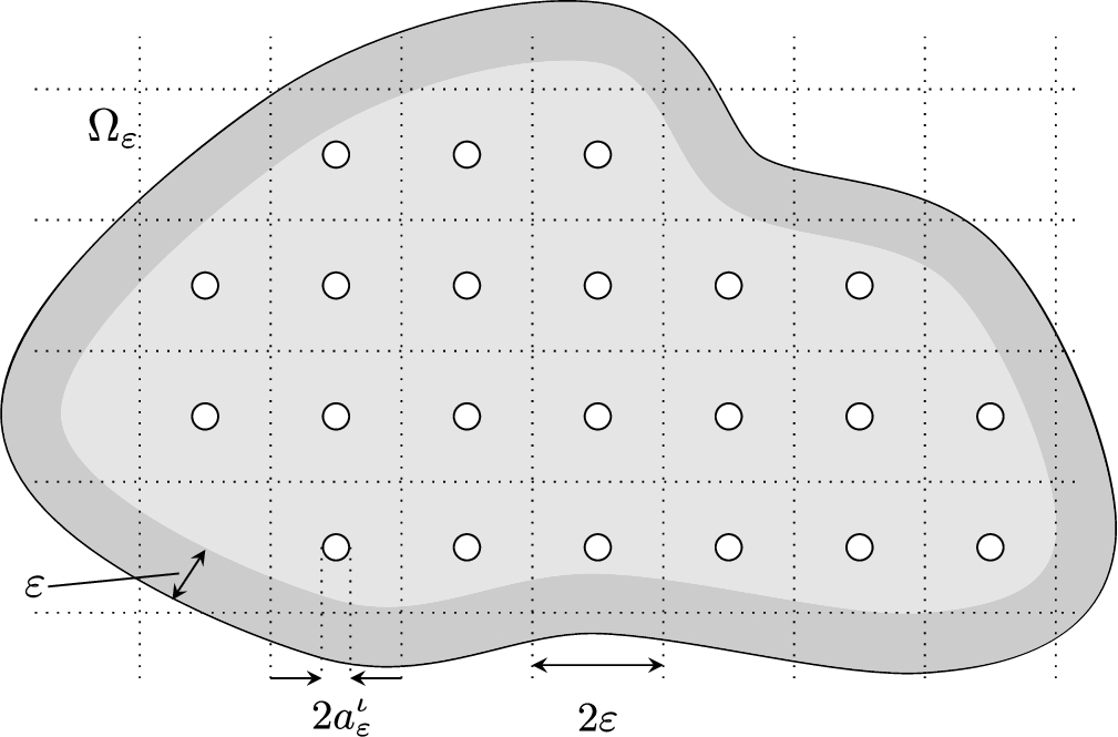Let $α \in C ∖ {0}, Re (α) ⩾ 0$ and denote $Ω_{ε} : = Ω ∖ ⋃_{i \in L_{ε}} B_{a_{ε}} (i)$ where $ε \in (0, 1)$ , $B_{a_{ε}} (i)$ is the ball of radius $\begin{matrix} (1.1) & a_{ε}^{D} = \{\begin{matrix} ε^{d / (d - 2)}, & d ⩾ 3, \\ e^{- 1 / ε^{2}}, & d = 2, \end{matrix} a_{ε}^{N} = o (ε) (ε \to 0), a_{ε}^{α} = ε^{d / (d - 1)} \end{matrix}$ centered at the point $i \in L_{ε}$ , and $\begin{matrix} (1.2) & L_{ε} : = {i \in 2 ε Z^{d} : dist (i, \partial Ω) > ε} . \end{matrix}$

Consider the boundary value problems (cf. Figure 1) $\begin{array}{l} (Dir) & \{\begin{matrix} (- Δ + 1) u^{ε} = f & in Ω_{ε}, \\ u^{ε} = 0 & on \partial Ω_{ε}, \end{matrix} \\ (Neu) & \{\begin{matrix} (- Δ + 1) u^{ε} = f & in Ω_{ε}, \\ \partial_{ν} u^{ε} = 0 & on \partial Ω_{ε}, \end{matrix} \\ (Rob) & \{\begin{matrix} (- Δ + 1) u^{ε} = f & in Ω_{ε}, \\ \partial_{ν} u^{ε} + α u = 0 & on \partial Ω_{ε}, \end{matrix} \end{array}$ i.e. the resolvent problem for the Laplacian, subject to the Dirichlet, Neumann and Robin boundary conditions, respectively. It is easy to see, using the Lax–Milgram theorem, that for all $ε \in (0, 1)$ each of these problems has a unique weak solution $u^{ε}$ . It is a classical question, which we refer to as the homogenisation problem, whether the family of solutions to ( Dir ), ( Neu ), ( Rob ), obtained by varying the parameter ε, converges in the sense of the $L^{2}$ -norm to a function $u \in L^{2} (Ω)$ as $ε \to 0$ and whether the limit function u solves, in a reasonable sense, some PDE whose form is independent of the right-hand side datum f.

Fig. 1.

Sketch of the perforated domain.

Homogenisation problems of this type have been studied extensively for a long time [2,5,7,11]. For example, results by Cioranescu & Murat and Kaizu give a positive answer to the previous question for all three choices of boundary conditions at least in the case of bounded domains. In fact, they showed that the solutions of ( Dir ), ( Rob ), ( Neu ) converge strongly in $L^{2} (Ω)$ to the solution $u \in H^{1} (Ω)$ of $(- Δ + 1 + μ_{ι}) u = f$ , where $\begin{matrix} (1.3) & μ_{ι} = \{\begin{matrix} \frac{π}{2}, & ι = D, d = 2, \\ \frac{(d - 2) S_{d}}{2^{d}}, & ι = D, d ⩾ 3, \\ 0, & ι = N, \\ \frac{α S_{d}}{2^{d}}, & ι = α, \end{matrix} \end{matrix}$ where $S_{d}$ denotes the surface area of the unit ball in $R^{d}$ .

In this article we attempt to improve this result in two directions. First, we show the above convergence not only in the strong sense, but in the norm-resolvent sense (that is, the right-hand side f is allowed to depend on ε). Second, our result is then extended to the case of unbounded domains. As a corollary, we obtain a statement about the convergence of the spectra of the perforated domain problems ( Dir ), ( Neu ), ( Rob ) as $ε \to 0$ .

The paper is organised as follows. In Section 2 we will briefly give a more precise formulation of the problem and include previous results. In Section 3 we will state our main result and its implications. Sections 4, 5 and 6 contain the proof of the main theorem and in Section 7 we consider implications of our main theorem for the semigroup generated by the Robin Laplacian. Section 8 contains a brief conclusion and discusses open problems.

2. Geometric setting and previous results

As above, assume $d ⩾ 2$ , and let $\begin{matrix} T_{ε} : = ⋃_{i \in L_{ε}} T_{i}^{ε}, T_{i}^{ε} : = B_{a_{ε}^{ι}} (i), i \in L_{ε}, \end{matrix}$ where $a_{ε}^{ι}$ , $L_{ε}$ as in (1.1), (1.2). Denote $Ω_{ε} : = Ω ∖ T_{ε}$ . We also denote $B_{i}^{ε} : = B_{ε} (i)$ and $P_{i}^{ε} : = ε {[- 1, 1]}^{d} + i$ for $i \in L_{ε}$ . Constants independent of ε will be denoted C and may change from line to line. Note that our assumptions on Ω ensure that the set ${ϕ |_{Ω} : ϕ \in C_{0}^{\infty} (R^{d})}$ is dense in $H^{1} (Ω)$ (cf. [1, Cor. 9.8]) in the cases $ι = N, α$ .

Moreover, since we are dealing with varying spaces $L^{2} (Ω_{ε})$ , it is convenient to define the identification operators $\begin{array}{l} (2.1) & J_{ε} : L^{2} (Ω_{ε}) \to L^{2} (Ω), J_{ε} f (x) = \{\begin{matrix} f (x), & x \in Ω_{ε}, \\ 0, & x \in Ω ∖ Ω_{ε} \end{matrix} \\ (2.2) & I_{ε} : L^{2} (Ω_{ε}) \to L^{2} (Ω), I_{ε} g (x) = g |_{Ω_{ε}} \\ (2.3) & T_{ε} : H^{1} (Ω_{ε}) \to H^{1} (Ω), T_{ε} u = \{\begin{matrix} u & in Ω_{ε}, \\ v & in T_{ε}, \end{matrix} \end{array}$ where v is the harmonic extension of u into the holes, i.e. $\begin{matrix} (2.4) & \{\begin{matrix} Δ v = 0 & in T_{ε}, \\ v = u & on \partial T_{ε} . \end{matrix} \end{matrix}$

Lemma 2.1.
For $I_{ε}, J_{ε}$ as above, one has $\begin{array}{l} (2.5) & I_{ε} J_{ε} = {id}_{L^{2} (Ω_{ε})} \\ (2.6) & ‖ J_{ε} I_{ε} - {id}_{L^{2} (Ω)} ‖_{L (H^{1} (Ω), L^{2} (Ω))} \to 0 . \end{array}$ Moreover, $‖ I_{ε} ‖_{L (L^{2} (Ω_{ε}), L^{2} (Ω))}, ‖ J_{ε} ‖_{L (L^{2} (Ω), L^{2} (Ω_{ε}))}$ are uniformly bounded in ε.
Proof.
The only nontrivial statement is (2.6). To prove this, let $f \in H^{1} (Ω_{ε})$ . Then $‖ f - J_{ε} I_{ε} f ‖_{L^{2} (Ω)} = ‖ f ‖_{L^{2} (T_{ε})}$ . To show that this quantity converges to 0 uniformly in f, denote ${Q_{k} : = [0, 1)}^{d} + k$ for $k \in Z^{d}$ a cube shifted by k, so that $R^{d} = ⋃_{k \in Z^{d}} Q_{k}$ . Then we have $\begin{array}{l} ‖ f ‖_{L^{2} (T_{ε})}^{2} & = \sum_{k \in Z^{d}} ‖ f ‖_{L^{2} (Q_{k} \cap T_{ε})}^{2} \\ ⩽ \sum_{k \in Z^{d}} ‖ 1 ‖_{L^{2 p} (Q_{k} \cap T_{ε})}^{2} ‖ f ‖_{L^{2 q} (Q_{k} \cap T_{ε})}^{2} \end{array}$ for $p, q > 1$ with $p^{- 1} + q^{- 1} = 1$ , by Hölder’s inequality. Since $f \in H^{1} (Ω)$ , we can use the Gagliardo–Sobolev–Nierenberg inequality to conclude (for suitable q) that $\begin{array}{l} ‖ f ‖_{L^{2} (T_{ε})}^{2} & ⩽ ‖ 1 ‖_{L^{2 p} (Q_{0} \cap T_{ε})}^{2} \sum_{k \in Z^{d}} ‖ f ‖_{L^{2 q} (Q_{k} \cap T_{ε})}^{2} \\ ⩽ ‖ 1 ‖_{L^{2 p} (Q_{0} \cap T_{ε})}^{2} \sum_{k \in Z^{d}} C ‖ f ‖_{H^{1} (Q_{k} \cap T_{ε})}^{2} \\ = | Q_{0} \cap T_{ε} |^{1 / p} C ‖ f ‖_{H^{1} (T_{ε})}^{2} \end{array}$ with some suitable $p > 0$ . Since $| Q_{0} \cap T_{ε} | \to 0$ as $ε \to 0$ (cf. the definition of $a_{ε}^{ι}$ , (1.1)), the desired convergence follows. □
Lemma 2.2.
In the cases $ι \in {N, α}$ the harmonic extension operator $T_{ε}$ satisfies
${lim sup}_{ε \to 0} ‖ T_{ε} ‖_{H^{1} (Ω_{ε}) \to H^{1} (Ω)} < \infty$ .

There exists $C > 0$ such that $‖ T_{ε} w ‖_{H^{1} (P_{i}^{ε})} ⩽ C ‖ w ‖_{H^{1} (P_{i}^{ε})}$ for all $w \in H^{1} (Ω_{ε})$ and $i \in L_{ε}$ .

For any sequence $w_{ε}$ such that ${lim sup}_{ε \to 0} ‖ w_{ε} ‖_{H^{1} (Ω_{ε})} < \infty$ one has $‖ T_{ε} w_{ε} - J_{ε} w_{ε} ‖_{L^{2} (Ω)} \to 0$ .

Proof.
See [5], [11, p. 40]. □

In the above geometric setting, we will study the linear operators $A_{ε}^{ι}$ , $ι = D, N, α$ in $L^{2} (Ω_{ε})$ , defined by the differential expression $- Δ + 1$ , with (dense) domains $\begin{array}{l} D (A_{ε}^{D}) = H_{0}^{1} (Ω_{ε}) \cap H^{2} (Ω_{ε}), \\ D (A_{ε}^{N}) = {u \in H^{2} (Ω_{ε}) : \partial_{ν} u = 0 on \partial Ω_{ε}}, \\ D (A_{ε}^{α}) = {u \in H^{2} (Ω_{ε}) : \partial_{ν} u + α u = 0 on \partial Ω_{ε}}, \end{array}$ respectively, and the linear operators $A^{ι}$ in $L^{2} (Ω_{ε})$ defined by the expression $- Δ + 1 + μ_{ι}$ , with domains $\begin{array}{l} D (A^{D}) = H_{0}^{1} (Ω) \cap H^{2} (Ω), \\ D (A^{N}) = {u \in H^{2} (Ω) : \partial_{ν} u = 0 on \partial Ω}, \\ D (A^{α}) = {u \in H^{2} (Ω) : \partial_{ν} u + α u = 0 on \partial Ω}, \end{array}$ respectively, where $μ_{ι}$ , $ι = D, N, α$ , are defined in (1.3).
Remark 2.3.
In the case when $d ⩾ 3$ one has the characterisation $\begin{matrix} (2.7) & μ_{D} = \frac{1}{2^{d}} min {\int_{R^{d} ∖ B_{1} (0)} | \nabla u |^{2}, u \in H^{1} (R^{d}), u = 1 on B_{1} (0)} . \end{matrix}$ Note that the factor $1 / 2^{d}$ arises from the fact that the unit cell is of size $2 ε$ .

Using the notation above, we recall the following classical results.
Theorem 2.4 ([2]).

Let $Ω \subset R^{d}$ be open (bounded or unbounded). Suppose that $f \in L^{2} (Ω)$ , and let $u^{ε}$ and $\tilde{u}$ be the solutions to $\begin{array}{l} (- Δ + 1) u^{ε} = f, u^{ε} \in H_{0}^{1} (Ω_{ε}), \\ (- Δ + 1 + μ_{D}) \tilde{u} = f, \tilde{u} \in H_{0}^{1} (Ω) . \end{array}$ Then $J_{ε} u^{ε} \overset{ε \to 0}{⇀} \tilde{u}$ in $H_{0}^{1} (Ω)$ .

Theorem 2.5 ([5]).

Let $Ω \subset R^{d}$ be open (bounded or unbounded), and suppose that $\partial Ω$ is smooth. Suppose also that $f \in L^{2} (Ω)$ , and let $u^{ε}$ and $\tilde{u}$ be the solutions to $\begin{array}{l} (- Δ + 1) u^{ε} = f, u^{ε} \in D (A_{ε}^{α, N}), \\ (- Δ + 1 + μ_{α, N}) \tilde{u} = f, \tilde{u} \in D (A^{α, N}) . \end{array}$ Then one has $\begin{matrix} J_{ε} u^{ε} \overset{ε \to 0}{⇀} \tilde{u} in H^{1} (Ω) . \end{matrix}$

Proof of Theorems 2.4 and 2.5.
The results are obtained by following the proofs of [2, Thm 2.2], [5, Thm 2]. Note that the weak convergence in $H^{1} (Ω)$ is immediately obtained also for unbounded domains (and complex α). □

An important ingredient in the proofs are auxiliary functions $w_{ϵ}^{ι} \in W^{1, \infty} (R^{d})$ defined, for each $ε \in (0, 1)$ , as the solution to the problems $\begin{matrix} (2.8) & w_{ε}^{N} \equiv 1, \{\begin{matrix} w_{ε}^{D} = 0 & in T_{i}^{ε}, \\ Δ w_{ε}^{D} = 0 & in B_{i}^{ε} ∖ T_{i}^{ε}, \\ w_{ε}^{D} = 1 & in P_{i}^{ε} ∖ B_{i}^{ε}, \\ w_{ε}^{D} & continuous, \end{matrix} \{\begin{matrix} \partial_{ν} w_{ε}^{α} + α w_{ε}^{α} = 0 & on \partial T_{i}^{ε}, \\ Δ w_{ε}^{α} = 0 & in B_{i}^{ε} ∖ T_{i}^{ε}, \\ w_{ε}^{α} = 1 & in P_{i}^{ε} ∖ B_{i}^{ε}, \\ w_{ε}^{α} & continuous, \end{matrix} \end{matrix}$ used as a test function in the weak formulation of the problems ( Dir ), ( Neu ), ( Rob ).

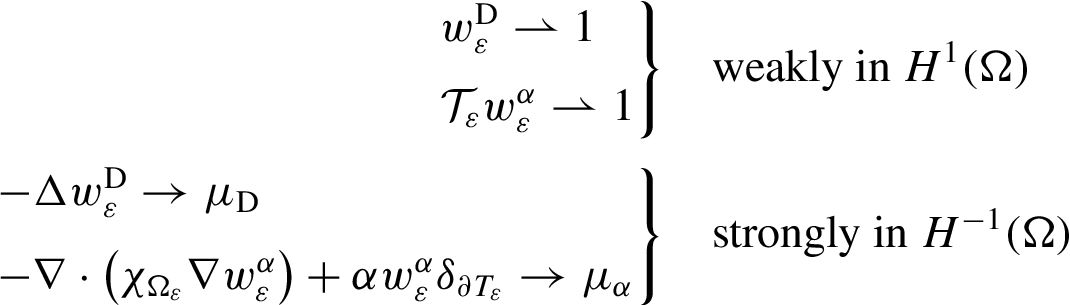
These functions were used in [2,5] as test functions to prove strong convergence of solutions. They are “optimal” in the sense that they minimise the energy in annular regions around the holes. In the Dirichlet case, the function $w_{ε}^{D}$ is nothing but the potential for the capacity $cap (B_{ε} (i); B_{a_{ε}^{D}} (i))$ . It can be shown that one has the convergences

as $ε \to 0$ , where $δ_{\partial T_{ε}}$ denotes the Dirac measure on the boundary of the holes (for a proof of the above facts, see [2, Lemma 2.3] and [5, Section 3]).
3. Main results

In what follows we prove the following claim.

Theorem 3.1.
Let $J_{ε}, A_{ε}^{ι}, A^{ι}$ be defined as in the previous section. Then for $ι \in {D, N, α}$ one has $\begin{array}{l} (3.1) & {‖ J_{ε} {(A_{ε}^{ι})}^{- 1} - {(A^{ι})}^{- 1} J_{ε} ‖}_{L (L^{2} (Ω_{ε}), L^{2} (Ω))} \to 0 (ε \to 0), \end{array}$ that is, the operator sequence $A_{ε}^{ι}$ converges to $A^{ι}$ in the norm-resolvent sense.
Corollary 3.2.
If $A_{ε}, A$ are as in Theorem 3.1 , then $\begin{array}{l} (3.2) & {‖ {(A_{ε}^{ι})}^{- 1} I_{ε} - I_{ε} {(A^{ι})}^{- 1} ‖}_{L (L^{2} (Ω), L^{2} (Ω_{ε}))} \to 0, \end{array}$ where $I_{ε}$ is as in ( 2.2 ).
Proof.
For notational convenience, denote $R_{ε} : = {(A_{ε}^{ι})}^{- 1}$ and $R : = {(A^{ι})}^{- 1}$ . A quick calculation shows that $\begin{array}{l} R_{ε} I_{ε} - I_{ε} R & = I_{ε} (J_{ε} R_{ε} - R J_{ε}) I_{ε} - (I_{ε} J_{ε} - 1) R_{ε} I_{ε} \\ = I_{ε} (J_{ε} R_{ε} - R J_{ε}) I_{ε}, \end{array}$ since $I_{ε} J_{ε} = {id}_{L^{2} (Ω_{ε})}$ . Hence $\begin{array}{l} ‖ R_{ε} I_{ε} - I_{ε} R ‖_{L (L^{2} (Ω), L^{2} (Ω_{ε}))} & ⩽ ‖ I_{ε} ‖_{L (L^{2} (Ω), L^{2} (Ω_{ε})}^{2} ‖ J_{ε} R_{ε} - R J_{ε} ‖_{L (L^{2} (Ω_{ε}), L^{2} (Ω))} \\ \to 0 \end{array}$ as $ε \to 0$ , by (3.1) and uniform boundedness of $‖ I_{ε} ‖_{L (L^{2} (Ω_{ε}), L^{2} (Ω))}$ . □

We note an important consequence of the above theorem.
Corollary 3.3.
For all compact $K \subset C$ , one has $σ (A_{ε}^{ι}) \cap K \overset{ε \to 0}{\to} σ (A^{ι}) \cap K$ in the Hausdorff sense. 1 ¹
For the definition of Hausdorff convergence, see e.g. [12].

Proof.
First, note that the spectra of $A_{ε}^{ι}$ converge to that of $A^{ι}$ , in the sense that for each compact $K \subset ρ (A^{ι})$ there exists $ε_{0} > 0$ such that $K \subset ρ (A_{ε}^{ι})$ for all $ε \in (0, ε_{0})$ . The proof of this is obtained by combining the proofs of Lemma 3.11, Theorem 3.12 and Corollary 3.14 in [8]. On the other hand, an analogous proof using (3.2) and (2.6) shows that if $K \subset ρ (A_{ε}^{ι})$ for almost all $ε > 0$ , then $K \subset ρ (A^{ι})$ . Together these two facts imply Hausdorff convergence. □

In particular, this corollary shows that (if $Re (μ_{ι}) > 0$ ) a spectral gap opens for $A_{ε}^{ι}$ between 0 and $Re (μ_{ι})$ . Remark 3.4.
We note that our assumption on the spherical shape of the holes was made for the sake of definiteness, however, our results easily generalise to more general geometries as detailed in [2, Th. 2.7]. Moreover, our results are also valid for more general elliptic operators $div (A \nabla)$ with continuous coefficients A (cf. [2]).

4. Uniformity with respect to the right-hand side

In this section we prove that the result of Theorems 2.4, 2.5 hold in a strengthened form, namely, uniformly with respect to the right-hand side f. More precisely, the following holds.

Theorem 4.1.
Suppose that $ε_{n} ↘ 0$ , $f_{n} \in L^{2} (Ω_{ε_{n}})$ , $n \in N$ , with $‖ f_{n} ‖_{L^{2} (Ω_{ε})} ⩽ 1$ , and let $u_{n}^{ι}$ and ${\tilde{u}}_{n}^{ι}$ be the solutions to the problems ( $ι \in {D, N, α}$ ) $\begin{array}{l} (4.1) & (- Δ + 1) u_{n}^{ι} = f_{n}, u_{n}^{ι} \in D (A_{ε_{n}}^{ι}), \\ (4.2) & (- Δ + 1 + μ_{ι}) {\tilde{u}}_{n}^{ι} = J_{ε_{n}} f_{n}, {\tilde{u}}_{n}^{ι} \in D (A^{ι}) . \end{array}$ Then for every bounded, open $K \subset Ω$ one has $\begin{array}{l} J_{ε_{n}} u_{n}^{ι} - {\tilde{u}}_{n}^{ι} \to 0 strongly in L^{2} (K), \\ J_{ε_{n}} \nabla u_{n}^{ι} - \nabla {\tilde{u}}_{n}^{ι} ⇀ 0 weakly in L^{2} (K), \end{array}$ for $ι \in {D, N, α}$ .
Proof.
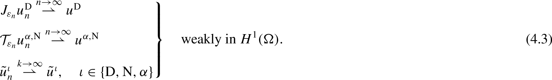
We have the following a priori estimates (note Lemma 2.2): $\begin{array}{l} {‖ T_{ε_{n}} u_{n}^{α, N} ‖}_{H^{1} (Ω)} ⩽ C ‖ J_{ε_{n}} f_{n} ‖_{L^{2} (Ω)}, \\ {‖ J_{ε_{n}} u_{n}^{D} ‖}_{H^{1} (Ω)} ⩽ C ‖ J_{ε_{n}} f_{n} ‖_{L^{2} (Ω)}, \\ {‖ {\tilde{u}}_{n}^{ι} ‖}_{H^{1} (Ω)} ⩽ C ‖ J_{ε_{n}} f_{n} ‖_{L^{2} (Ω)} \forall ι \in {D, N, α} . \end{array}$ Thus, there exists a subsequence (still indexed by n) and $u^{ι}, {\tilde{u}}^{ι} \in H^{1} (Ω)$ such that

Note that that for every bounded $K \subset Ω$ the convergence statements (4.3) are strong in $L^{2} (K)$ . In particular, employing Lemma 2.2(i), (iii) and the Rellich Theorem we immediately obtain $\begin{array}{l} J_{ε_{n}} u_{n}^{ι} \to u^{ι} strongly in L^{2} (K), \\ J_{ε_{n}} \nabla u_{n}^{ι} ⇀ \nabla u^{ι} weakly in L^{2} (K) \\ (4.4) & {\tilde{u}}_{n}^{ι} ⇀ {\tilde{u}}^{ι} strongly in L^{2} (K), \\ (4.5) & \nabla {\tilde{u}}_{n}^{ι} ⇀ \nabla {\tilde{u}}^{ι} weakly in L^{2} (K) . \end{array}$ for all $ι \in {D, N, α}$ . Next, choose a further subsequence (still indexed by n) such that also $J_{ε_{n}} f_{n} \overset{n \to \infty}{⇀} f$ weakly in $L^{2} (Ω)$ , where the limit f may depend on the choice of subsequence. Now, consider the weak formulations of the problem (4.2), i.e. $\begin{array}{l} \int_{Ω} \overline{\nabla {\tilde{u}}_{n}^{ι}} \nabla ϕ + (1 + μ_{ι}) \int_{Ω} \overline{{\tilde{u}}_{n}^{ι}} ϕ = \int_{Ω} \overline{f_{n}} ϕ, \end{array}$ where $ϕ \in C_{0}^{\infty} (Ω)$ for $ι = D$ and $ϕ \in C_{0}^{\infty} (R^{d})$ for $ι = α, N$ . Letting $n \to \infty$ and using the convergencies (4.4), (4.5) (with $K = Ω \cap supp ϕ$ ) we obtain $\begin{array}{l} \int_{Ω} \overline{\nabla {\tilde{u}}^{ι}} \nabla ϕ + (1 + μ_{ι}) \int_{Ω} \overline{{\tilde{u}}^{ι}} ϕ = \int_{Ω} \overline{f} ϕ . \end{array}$ Next consider the weak formulation of (4.1),where we choose the test function $w_{ε_{n}}^{ι} ϕ$ : $\begin{array}{l} \int_{Ω_{ε_{n}}} \overline{\nabla u_{n}^{ι}} \nabla (w_{ε_{n}}^{ι} ϕ) + \int_{Ω_{ε_{n}}} \overline{u_{n}^{ι}} w_{ε_{n}}^{ι} ϕ = \int_{Ω_{ε_{n}}} \overline{f_{n}} w_{ε_{n}}^{ι} ϕ, \end{array}$ where again $ϕ \in C_{0}^{\infty} (Ω)$ for $ι = D$ and $ϕ \in C_{0}^{\infty} (R^{d})$ for $ι = α, N$ . It follows from the results of [2,5] that the left and right-hand side of this equation converge to $\begin{matrix} \int_{Ω} (\overline{\nabla u^{ι}} \nabla ϕ + (1 + μ_{ι}) \overline{u^{ι}} ϕ) and \int_{Ω} \overline{f} ϕ, \end{matrix}$ respectively. Thus, we obtain $\begin{matrix} \int_{Ω} (\overline{\nabla u^{ι}} \nabla ϕ + (1 + μ_{ι}) \overline{u^{ι}} ϕ) = \int_{Ω} \overline{f} ϕ, \end{matrix}$ and hence $u^{ι}$ and ${\tilde{u}}^{ι}$ are weak solutions to the same equation. Uniqueness of solutions (for all $ι \in {D, N, α}$ ) implies ${\tilde{u}}^{ι} = u^{ι}$ , which shows the assertion for the chosen subsequence.

Finally, applying the above reasoning to every subsequence of $(J_{ε_{n}} u_{n}^{ι} - {\tilde{u}}_{n}^{ι})$ yields the result for the whole sequence. □
Corollary 4.2.
If the domain Ω is bounded, one has $\begin{matrix} {‖ J_{ε} {(A_{ε}^{ι})}^{- 1} - {(A^{ι})}^{- 1} J_{ε} ‖}_{L (L^{2} (Ω_{ε}), L^{2} (Ω))} \to 0 (ε \to 0) \end{matrix}$ for $ι \in {D, N, α}$ , i.e., Theorem 3.1 holds in that case of bounded Ω.
Proof.
Since Ω is bounded, the embedding of $H^{1} (Ω)$ in $L^{2} (Ω)$ is compact, thus the sequence $J_{ε_{n}} u_{n}^{ι} - {\tilde{u}}_{n}^{ι}$ from the previous proof has a subsequence converging to 0 strongly in $L^{2} (Ω)$ . Since this can be done for every subsequence of $(J_{ε_{n}} u_{n}^{ι} - {\tilde{u}}_{n}^{ι})$ , the whole sequence converges to 0.

Now, choose a sequence $f_{n} \in L^{2} (Ω_{ε_{n}}), ‖ f_{n} ‖_{L^{2} (Ω_{ε})} ⩽ 1$ , such that $\begin{array}{l} sup_{\begin{array}{c} f \in L^{2} (Ω_{ε_{n}}) \\ ‖ f ‖ ⩽ 1 \end{array}} {‖ (J_{ε_{n}} {(A_{ε}^{ι})}^{- 1} - {(A^{ι})}^{- 1} J_{ε_{n}}) f ‖}_{L^{2} (Ω_{ε})} - \frac{1}{n} \\ < {‖ (J_{ε_{n}} {(A_{ε_{n}}^{ι})}^{- 1} - {(A^{ι})}^{- 1} J_{ε_{n}}) f_{n} ‖}_{L^{2} (Ω_{ε_{n}})} . \end{array}$ By the above, the right-hand side of this inequality converges to zero, which implies the claim. □

Treating unbounded domains requires further effort. Since we lack compact embeddings in this case, we will have to take advantage of the sufficiently rapid decay of solutions to $(- Δ + 1) u = f$ and a decomposition of the right hand side with a bound on the interactions.
5. Exponential decay of solutions

We begin with a general result which we assume is classical, but include for the sake of completeness. Let $U \subset R^{d}$ open satisfying the strong local Lipschitz condition, $λ > \frac{1}{2}$ and consider the problems (cf. ( Dir ), ( Neu ), ( Rob )) $\begin{array}{l} (5.1) & \{\begin{matrix} (- Δ + λ) u^{α} = f & in U, \\ \partial_{ν} u^{α} + α u^{α} = 0 & on \partial U; \end{matrix} \\ (5.2) & \{\begin{matrix} (- Δ + λ) u^{N} = f & in U, \\ \partial_{ν} u^{N} = 0 & on \partial U; \end{matrix} \\ (5.3) & \{\begin{matrix} (- Δ + λ) u^{D} = f & in U, \\ u^{D} = 0 & on \partial U . \end{matrix} \end{array}$ Let $x_{0} \in R^{d}$ , and define the function $ω (x) = cosh (| x - x_{0} |)$ . Then the following statement holds.

Proposition 5.1.
Let $f \in L^{2} (U)$ , $supp (f)$ compact. Then each of the problems ( 5.1 )–( 5.3 ) has a unique weak solution $u^{ι} \in H^{1} (U)$ satisfying $\begin{array}{l} (5.4) & \int_{U} {| u^{ι} |}^{2} ω d x ⩽ M \int_{U} | f |^{2} ω d x \\ (5.5) & \int_{U} {| \nabla u^{ι} |}^{2} ω d x ⩽ M \int_{U} | f |^{2} ω d x, \end{array}$ where $M : = max {2, {(λ - \frac{1}{2})}^{- 1}}$ .

We postpone the proof, in order to introduce some notation and prove auxiliary results. First, let us denote $d μ : = ω d x$ and introduce the weighted Sobolev spaces $H : = W^{1, 2} (U; ω)$ , $H_{0} : = W_{0}^{1, 2} (U; ω)$ with scalar product $\begin{matrix} {⟨ u, v ⟩}_{H} = \int_{U} u v d μ + \int_{U} \nabla u \cdot \nabla v d μ . \end{matrix}$ Moreover, let $λ > \frac{1}{2}$ and define the sesquilinear forms $\begin{array}{l} (5.6) & a^{α} (u, v) : = \int_{U} (\overline{\nabla u} \cdot \nabla v + λ \overline{u} v) d μ + \int_{U} v \overline{\nabla u} \cdot \frac{\nabla ω}{ω} d μ + α \int_{\partial U} \overline{u} v ω d S on H, \\ (5.7) & a^{N} (u, v) : = \int_{U} (\overline{\nabla u} \cdot \nabla v + λ \overline{u} v) d μ + \int_{U} v \overline{\nabla u} \cdot \frac{\nabla ω}{ω} d μ on H, \\ (5.8) & a^{D} (u, v) : = \int_{U} (\overline{\nabla u} \cdot \nabla v + λ \overline{u} v) d μ + \int_{U} v \overline{\nabla u} \cdot \frac{\nabla ω}{ω} d μ on H_{0} . \end{array}$ Lemma 5.2.
For $λ > \frac{1}{2}$ and $ι \in {D, N, α}$ , the form $a^{ι}$ is continuous and coercive on $H$ (on $H_{0}$ in the case $ι = D$ ).
Proof.
We will only treat the Robin case here, the other cases being analogous. Denote by I the second term in (5.6) and note that ω was chosen so that $| \nabla ω | ⩽ ω$ . By Hölder’s inequality with respect to μ one has $\begin{array}{l} | I | ⩽ \underset{⩽ 1}{\underset{︸}{{‖ \frac{\nabla ω}{ω} ‖}_{\infty}}} ‖ \nabla u ‖_{L^{2} (μ)} ‖ v ‖_{L^{2} (μ)} ⩽ \frac{1}{2} ‖ \nabla u ‖_{L^{2} (μ)}^{2} + \frac{1}{2} ‖ v ‖_{L^{2} (μ)}^{2}, \end{array}$ and thus $\begin{array}{l} | a (u, u) | & ⩾ ‖ \nabla u ‖_{L^{2} (μ)}^{2} + λ ‖ u ‖_{L^{2} (μ)}^{2} + | α | {‖ ω^{1 / 2} u ‖}_{L^{2} (\partial U)}^{2} + I \\ ⩾ ‖ \nabla u ‖_{L^{2} (μ)}^{2} + λ ‖ u ‖_{L^{2} (μ)}^{2} - \frac{1}{2} ‖ \nabla u ‖_{L^{2} (μ)}^{2} - \frac{1}{2} ‖ u ‖_{L^{2} (μ)}^{2} \\ = \frac{1}{2} ‖ \nabla u ‖_{L^{2} (μ)}^{2} + (λ - \frac{1}{2}) ‖ u ‖_{L^{2} (μ)}^{2}, \end{array}$ which shows coercivity in $H$ . Continuity follows by estimating the boundary term. By the trace theorem [3, Prop. IX.18.1] we have, for each $δ > 0$ , $\begin{array}{l} (5.9) & \int_{\partial U} | u |^{2} ω d x & ⩽ 2 δ {‖ \nabla (ω^{1 / 2} u) ‖}_{L^{2} (U)}^{2} + \frac{C}{δ} {‖ ω^{1 / 2} u ‖}_{L^{2} (U)}^{2} . \end{array}$ The first term can be estimated using the special choice of ω: $\begin{array}{l} {‖ \nabla (ω^{1 / 2} u) ‖}_{L^{2} (U)}^{2} & = \int_{U} {| ω^{1 / 2} \nabla u + \frac{1}{2} u \frac{\nabla ω}{ω^{1 / 2}} |}^{2} d x \\ ⩽ 2 \int_{U} ω | \nabla u |^{2} d x + \frac{1}{2} \int_{U} | u |^{2} \frac{| \nabla ω |^{2}}{ω} d x \\ ⩽ 2 ‖ \nabla u ‖_{L^{2} (μ)} + 2 {‖ \frac{\nabla ω}{ω} ‖}_{\infty}^{2} \int_{U} | u |^{2} ω d x \\ (5.10) & ⩽ 2 ‖ \nabla u ‖_{H^{1} (μ)}^{2} . \end{array}$ The desired continuity now follows immediately by combining (5.9) and (5.10). □
Lemma 5.3.
Let $f \in L^{2} (U)$ , $ι \in {D, N, α}$ , and suppose that $supp (f)$ is compact. Then the problem $\begin{matrix} (5.11) & a^{ι} (u, v) = \int_{U} \overline{f} v d μ \forall v \in H \end{matrix}$ has a solution in $H$ .
Proof.
By Hölder inequality, one has $\begin{matrix} | \int_{U} \overline{f} v d μ | ⩽ ‖ f ‖_{L^{2} (μ)} ‖ v ‖_{L^{2} (μ)} ⩽ ‖ ω ‖_{L^{\infty} (supp f)} ‖ f ‖_{L^{2} (U)} ‖ v ‖_{L^{2} (μ)}, \end{matrix}$ so $f \in H^{'}$ . The assertion now follows from Lemma 5.2 and the Lax–Milgram theorem for complex, non-symmetric sesquilinear forms [13, Thm. VI.1.4]. □
Proof of Proposition 5.1.
Again we focus on the Robin case, the other cases being analogous. Denote by u the solution obtained from Lemma 5.3. Then $u \in H^{1} (U)$ , since $H \subset H^{1} (U)$ . Moreover, let $ϕ \in C_{0}^{\infty} (R^{d})$ be arbitrary and decompose it as $ϕ = ω ψ$ . Then $ψ \in C_{0}^{\infty} (R^{d}) \subset H$ and one has $\begin{array}{l} \int_{U} \overline{\nabla u} \cdot \nabla ϕ d x + λ \int_{U} \overline{u} ϕ d x + α \int_{\partial U} \overline{u} ϕ d S \\ = \int_{U} \overline{\nabla u} \cdot (ω \nabla ψ + ψ \nabla ω) d x + λ \int_{U} \overline{u} ψ ω d x + α \int_{\partial U} \overline{u} ψ ω d S \\ = a^{α} (u, ψ) \\ = \int_{U} \overline{f} ψ d μ \\ = \int_{U} \overline{f} ϕ d x . \end{array}$ Thus, the function u solves the problem $\begin{matrix} (5.12) & \int_{U} \overline{\nabla u} \cdot \nabla ϕ d x + λ \int_{U} \overline{u} ϕ d x + α \int_{\partial U} \overline{u} ϕ d S = \int_{U} \overline{f} ϕ d x \forall ϕ \in C_{0}^{\infty} (R^{d}) . \end{matrix}$ Uniqueness of solutions and density of $C_{0}^{\infty} (R^{d})$ in $H^{1} (U)$ implies that u is the weak solution in $H^{1} (U)$ to the Robin problem (5.1).

The estimates (5.4), (5.5) follow from the coercivity of $a^{ι}$ . □

6. Decomposition of the right-hand side

In this section we consider the case of unbounded Ω. We conclude the proof of Theorem 3.1 by decomposing the domain into cubes $Q_{i}$ , writing $f = \sum_{i} f χ_{Q_{i}}$ and then applying the above results to each term $f χ_{Q_{i}}$ . The following lemma shows uniform convergence with respect to the position of the cubes.

Lemma 6.1.
Let $ε_{n} ↘ 0$ and $f_{n} \in L^{2} (Ω)$ , $n \in N$ , be such that $‖ f_{n} ‖_{L^{2} (Ω)} ⩽ 1$ and $supp (f_{n}) \subset Q_{i_{n}}$ , where $Q_{i_{n}} = {[0, 1]}^{d} + i_{n}$ with $i_{n} \in Z^{d}$ . Let $u_{n}^{ι}, {\tilde{u}}_{n}^{ι}$ be the solutions to the problems $\begin{array}{l} (6.1) & A_{ε_{n}}^{ι} u_{n}^{ι} = f_{n} |_{Ω_{ε_{n}}}, A^{ι} {\tilde{u}}_{n}^{ι} = f_{n}, n \in N, ι \in {D, N, α} . \end{array}$ Then $‖ J_{ε_{n}} u_{n}^{ι} - {\tilde{u}}_{n}^{ι} ‖_{L^{2} (Ω)} \to 0$ for all $ι \in {D, N, α}$ .
Proof.
The idea of the proof is to use translation invariance, in order to shift $supp (f_{n})$ back near zero for every n, and then use the Fréchet–Kolmogorov compactness criterion to obtain a convergent subsequence of $(J_{ε_{n}} u_{n}^{ι} - {\tilde{u}}_{n}^{ι})$ ; Theorem 4.1 will identify its limit as zero. Since the following analysis is independent of the choice of boundary conditions, we henceforth omit ι to simplify notation.

We now carry out the outlined strategy. We set, for all $n \in N$ , $\begin{array}{l} u_{n}^{} (x) : = u_{n} (x + i_{n}), {\tilde{u}}_{n}^{} (x) : = {\tilde{u}}_{n} (x + i_{n}), f_{n}^{} (x) : = f_{n} (x + i_{n}) . \end{array}$

These functions still solve the problems (6.1) with $f_{n}$ replaced by $f_{n}^{}$ and Ω replaced by $Ω - i_{n}$ . The new sequence $f_{n}^{}$ has the nice property that $supp (f_{n}^{}) \subset {[0, 1]}^{d}$ for all n. In the following we consider $J_{ε_{n}} u_{n}^{}, {\tilde{u}}_{n}^{}, f_{n}^{}$ as elements of $L^{2} (R^{d})$ that are zero outside $Ω - i_{n}$ . We will now show that ${\tilde{u}}_{n}^{} - J_{ε_{n}} u_{n}^{}$ converges to zero in $L^{2} (R^{d})$ . To this end, consider the bounded set $\begin{matrix} (6.2) & F : = {{\tilde{u}}_{n}^{} - J_{ε_{n}} u_{n}^{} : n \in N} \subset L^{2} (R^{d}) . \end{matrix}$

Claim: $F$ is precompact in $L^{2} (R^{d})$ .

We postpone the proof of this claim to Lemma 6.2. We immediately obtain that $({\tilde{u}}_{n}^{} - J_{ε_{n}} u_{n}^{})$ has a convergent subsequence in $L^{2} (R^{d})$ . Furthermore, Theorem 4.1 shows that $‖ {\tilde{u}}_{n}^{} - J_{ε_{n}} u_{n}^{} ‖_{L^{2} (K)} \to 0$ for every bounded $K \subset R^{d}$ which identifies the limit of the subsequence as zero.

Arguing as above for all subsequences of $({\tilde{u}}_{n}^{} - J_{ε_{n}} u_{n}^{})$ , we conclude that ${\tilde{u}}_{n}^{} - J_{ε_{n}} u_{n}^{} \to 0$ in $L^{2} (R^{d})$ . Since the shift $u \mapsto u (\cdot + i_{n})$ is an isometry in $L^{2} (R^{d})$ , this implies that ${\tilde{u}}_{n} - J_{ε_{n}} u_{n} \to 0$ in $L^{2} (Ω)$ . □
Lemma 6.2.
The set $F$ defined in ( 6.2 ) is precompact in $L^{2} (R^{d})$ .
Proof.
We will use the notation and conventions from the previous proof and distinguish between the Dirichlet case and the Robin/Neumann cases.

Dirichlet case. Step 1: We have $\begin{matrix} sup_{n} {‖ τ_{h} ({\tilde{u}}_{n}^{} - J_{ε_{n}} u_{n}^{}) - ({\tilde{u}}_{n}^{} - J_{ε_{n}} u_{n}^{}) ‖}_{L^{2} (R^{d})} \to 0 as h \to 0 \forall n \in N, \end{matrix}$ where $τ_{h}$ denotes the operator of translation by h. Indeed, the standard regularity theory implies $\begin{array}{l} {‖ τ_{h} ({\tilde{u}}_{n}^{} - J_{ε_{n}} u_{n}^{}) - ({\tilde{u}}_{n}^{} - J_{ε_{n}} u_{n}^{}) ‖}_{L^{2} (R^{d})} ⩽ {‖ \nabla ({\tilde{u}}_{n}^{} - J_{ε_{n}} u_{n}^{}) ‖}_{L^{2} (R^{d})} | h | ⩽ C ‖ f_{n} ‖_{L^{2} (Ω)} | h | . \end{array}$

Step 2: Notice that $\begin{array}{l} sup_{n} {‖ {\tilde{u}}_{n}^{} - J_{ε_{n}} u_{n}^{} ‖}_{L^{2} (R^{d} ∖ B_{R} (0))} \to 0 as R \to \infty, \end{array}$ due to the following estimate in which we set $ω_{0} (x) : = cosh (| x |)$ . $\begin{array}{l} {‖ {\tilde{u}}_{n}^{} - J_{ε_{n}} u_{n}^{} ‖}_{L^{2} (R^{d} ∖ B_{R} (0))}^{2} & ⩽ 2 {‖ {\tilde{u}}_{n}^{} ω_{0} ω_{0}^{- 1} ‖}_{L^{2} (Ω ∖ B_{R} (0))}^{2} + 2 {‖ J_{ε} u_{n}^{} ω_{0} ω_{0}^{- 1} ‖}_{L^{2} ((R^{d} ∖ B_{R} (0))}^{2} \\ ⩽ 4 M {‖ f_{n}^{} ω_{0} ‖}_{L^{2} (R^{d})}^{2} {‖ ω_{0}^{- 1} ‖}_{L^{\infty} (R^{d} ∖ B_{R} (0))}^{2} \\ \overset{Prop. 5.1}{} & ⩽ C ‖ f_{n} ‖_{L^{2} (Ω)}^{2} exp (- R) \end{array}$ which completes Step 2. Applying the Fréchet–Kolmogorov theorem yields the precompactness of $F$ .

Neumann and Robin case. Here the strategy is the same, but matters are complicated by the fact that $J_{ε_{n}} u_{n}^{}$ is not in $H^{1} (R^{d})$ . To show that $F$ is precompact, we decompose elements in $F$ as $\begin{array}{l} {\tilde{u}}_{n}^{} - J_{ε_{n}} u_{n}^{} = ({\tilde{u}}_{n}^{} - T_{ε_{n}} u_{n}^{}) + (T_{ε_{n}} - J_{ε_{n}}) u_{n}^{}, \end{array}$ define $F_{1} : = {{\tilde{u}}_{n}^{} - T_{ε_{n}} u_{n}^{} : n \in N}$ , $F_{2} : = {(T_{ε_{n}} - J_{ε_{n}}) u_{n}^{} : n \in N}$ and show that $F_{1}$ and $F_{2}$ are precompact in $L^{2} (R^{d})$ . We will begin by showing that $F_{1}$ is precompact. To this end, denote by $E : H^{1} (Ω) \to H^{1} (R^{d})$ an extension operator satisfying $E u |_{Ω} = u$ and $‖ E u ‖_{H^{1} (R^{d})} ⩽ C ‖ u ‖_{H^{1} (Ω)}$ for all $u \in H^{1} (Ω)$ (cf. Prop. VII.19.1 and Remark VII.19.2 in [3]). Note that by translation invariance one has $E τ_{h} = τ_{h} E$ and ${(E u_{n})}^{} = E (u_{n}^{})$ . We start by proving that $\begin{array}{l} sup_{n} {‖ τ_{h} E ({\tilde{u}}_{n}^{} - T_{ε_{n}} u_{n}^{}) - E ({\tilde{u}}_{n}^{} - T_{ε_{n}} u_{n}^{}) ‖}_{2} \to 0 as h \to 0 \end{array}$ This readily follows from the estimate $\begin{array}{l} {‖ τ_{h} E ({\tilde{u}}_{n}^{} - T_{ε_{n}} u_{n}^{}) - E ({\tilde{u}}_{n}^{} - T_{ε_{n}} u_{n}^{}) ‖}_{L^{2} (R^{d})} & ⩽ {‖ \nabla E ({\tilde{u}}_{n}^{} - T_{ε_{n}} u_{n}^{}) ‖}_{L^{2} (R^{d})} | h | \\ ⩽ C {‖ {\tilde{u}}_{n}^{} - T_{ε_{n}} u_{n}^{} ‖}_{H^{1} (Ω + i_{n})} | h | \\ ⩽ C {‖ f_{n}^{} ‖}_{L^{2} (Ω + i_{n})} | h | \\ ⩽ C | h | . \end{array}$ Next we prove that $\begin{array}{l} sup_{n} {‖ E ({\tilde{u}}_{n}^{} - T_{ε_{n}} u_{n}^{}) ‖}_{L^{2} (R^{d} ∖ B_{R} (0))} \to 0 as R \to \infty . \end{array}$ Indeed, notice first that $\begin{array}{l} {‖ E ({\tilde{u}}_{n}^{} - T_{ε_{n}} u_{n}^{}) ‖}_{L^{2} (R^{d} ∖ B_{R} (0))}^{2} & ⩽ C ({‖ {\tilde{u}}_{n}^{} ‖}_{L^{2} ((Ω - i_{n}) ∖ B_{R} (0))}^{2} + {‖ T_{ε_{n}} u_{n}^{} ‖}_{L^{2} ((Ω_{ε_{n}} - i_{n}) ∖ B_{R} (0))}^{2}) \\ (6.3) & = C (‖ {\tilde{u}}_{n} ‖_{L^{2} (Ω ∖ B_{R} (i_{n}))}^{2} + ‖ T_{ε_{n}} u_{n} ‖_{L^{2} ((Ω_{ε_{n}}) ∖ B_{R} (i_{n}))}^{2}), \end{array}$ To treat the two terms on the right-hand side we apply Lemma 2.2(ii) and Proposition 5.1 with $ω_{i_{n}} (x) = cosh (| x + i_{n} |)$ as follows. For the second term in (6.3), we obtain $\begin{array}{l} ‖ T_{ε_{n}} u_{n} ‖_{L^{2} (Ω_{ε_{n}} ∖ B_{R} (i_{n}))} & ⩽ C (‖ u_{n} ‖_{L^{2} (Ω ∖ B_{R / 2} (i_{n}))} + ‖ \nabla u_{n} ‖_{L^{2} (Ω ∖ B_{R / 2} (i_{n}))}) \\ ⩽ {‖ ω_{i_{n}}^{1 / 2} ω_{i_{n}}^{- 1 / 2} u_{n} ‖}_{L^{2} (Ω ∖ B_{R / 2} (i_{n}))} + {‖ ω_{i_{n}}^{1 / 2} ω_{i_{n}}^{- 1 / 2} \nabla u_{n} ‖}_{L^{2} (Ω ∖ B_{R / 2} (i_{n}))} \\ ⩽ C ({‖ ω_{i_{n}}^{1 / 2} u_{n} ‖}_{L^{2} (Ω ∖ B_{R / 2} (i_{n}))} + {‖ ω_{n}^{1 / 2} \nabla u_{n} ‖}_{L^{2} (Ω ∖ B_{R / 2} (i_{n}))}) {‖ ω_{i_{n}}^{- 1 / 2} ‖}_{L^{\infty} (Ω ∖ B_{R / 2} (i_{n}))} \\ ⩽ C M {‖ f_{n} ω_{i_{n}}^{1 / 2} ‖}_{L^{2} (Ω)} exp (- R / 3) \\ ⩽ 2 C M exp (- R / 3), \end{array}$ where we use the fact that $ω_{i_{n}}$ is bounded by 2 on $supp f_{n}$ . With an analogous calculation for the first term in (6.3), we finally find $\begin{matrix} (6.4) & {‖ E ({\tilde{u}}_{n}^{} - T_{ε_{n}} u_{n}^{}) ‖}_{L^{2} (R^{d} ∖ B_{R} (0))} ⩽ C exp (- R / 3), \end{matrix}$ with C independent of n. Applying the Fréchet–Kolmogorov theorem yields the precompactness of the set ${E ({\tilde{u}}_{n}^{} - T_{ε_{n}} u_{n}^{}) : n \in N}$ . Finally, noting that $F_{1} = {E ({\tilde{u}}_{n}^{} - T_{ε_{n}} u_{n}^{}) : n \in N} χ_{Ω}$ and that multiplication by $χ_{Ω}$ is a bounded operator on $L^{2} (R^{d})$ we obtain precompactness of $F_{1}$ .

To prove precompactness of $F_{2}$ , first note that by Lemma 2.2(iii) for any $δ > 0$ there exists a $n_{0}$ such that $\begin{array}{l} {‖ (J_{ε_{n}} - T_{ε_{n}}) u_{n}^{} ‖}_{2} < δ \forall n > n_{0} . \end{array}$ Let us fix arbitrary $δ > 0$ and $n_{0}$ as above. It remains to estimate the terms $\begin{matrix} {‖ τ_{h} (J_{ε_{n}} - T_{ε_{n}}) u_{n}^{} - (J_{ε_{n}} - T_{ε_{n}}) u_{n}^{} ‖}_{L^{2} (R^{d})}, n ⩽ n_{0}, \end{matrix}$ but these are only finitely many, which clearly converge to zero individually, and hence $\begin{matrix} sup_{n ⩽ n_{0}} {‖ τ_{h} (J_{ε_{n}} - T_{ε_{n}}) u_{n}^{} - (J_{ε_{n}} - T_{ε_{n}}) u_{n}^{} ‖}_{2} \to 0 as h \to 0 \end{matrix}$ Altogether we have shown that $\begin{array}{l} sup_{n} {‖ τ_{h} (J_{ε_{n}} - T_{ε_{n}}) u_{n}^{} - (J_{ε_{n}} - T_{ε_{n}}) u_{n}^{} ‖}_{L^{2} (R^{d})} & = max {sup_{n ⩽ n_{0}} {‖ τ_{h} (J_{ε_{n}} - T_{ε_{n}}) u_{n}^{} - (J_{ε_{n}} - T_{ε_{n}}) u_{n}^{} ‖}_{2}, 2 δ} \\ \overset{h \to 0}{\to} 2 δ . \end{array}$ Since $δ > 0$ was arbitrary we finally get $\begin{array}{l} lim_{h \to 0} sup_{n \in N} {‖ τ_{h} (J_{ε_{n}} - T_{ε_{n}}) u_{n}^{} - (J_{ε_{n}} - T_{ε_{n}}) u_{n}^{} ‖}_{L^{2} (R^{d})} = 0 . \end{array}$ This completes the first Fréchet–Kolmogorov-condition. The proof of the second condition $\begin{array}{l} sup_{n} {‖ (J_{ε_{n}} - T_{ε_{n}}) u_{n}^{} ‖}_{L^{2} (R^{d} ∖ B_{R} (0))} \to 0 as R \to \infty \end{array}$ is analogous to the case of $F_{1}$ . Applying the Fréchet–Kolmogorov theorem yields precompactness of $F_{1}$ and completes the proof. □
Corollary 6.3.
There exists $δ_{ε}$ with $δ_{ε} \overset{ε \to 0}{⟶} 0$ such that $\begin{matrix} {‖ (J_{ε} {(A^{ι})}^{- 1} - {(A_{ε}^{ι})}^{- 1} J_{ε}) (f χ_{Q_{i} \cap Ω_{ε}}) ‖}_{L^{2} (Ω)} ⩽ δ_{ε} ‖ f χ_{Q_{i}} ‖_{L^{2} (Ω)} \end{matrix}$ for all $f \in L^{2} (Ω)$ and $i \in Z^{d}$ .
Proof.
We argue by contradiction. Suppose that there is no such function $δ_{ε}$ . Then there exist sequences $ε_{n}, f_{n}, i_{n}$ with $‖ f_{n} ‖_{L^{2} (Ω)} = 1$ such that $‖ (J_{ε} {(A^{ι})}^{- 1} - {(A_{ε_{n}}^{ι})}^{- 1} J_{ε}) (f_{n} χ_{Q_{i_{n}} \cap Ω_{ε_{n}}}) ‖_{L^{2} (Ω)}$ does not converge to zero, which is a contradiction to Lemma 6.1. □

In order to finalise the decomposition, we require he following two lemmas.
Lemma 6.4.
Suppose that $f \in L^{2} (Ω)$ , and denote $\begin{matrix} u_{i} : = (J_{ε} {(A^{ι})}^{- 1} - {(A_{ε}^{ι})}^{- 1} J_{ε}) (f χ_{Q_{i} \cap Ω_{ε}}), i \in Z^{d} . \end{matrix}$ Then one has $\begin{matrix} (6.5) & | {⟨ u_{i}, u_{j} ⟩}_{L^{2} (Ω)} | ⩽ C ‖ f χ_{Q_{i}} ‖_{L^{2} (Ω)} ‖ f χ_{Q_{j}} ‖_{L^{2} (Ω)} exp (- | i - j | / 2) \end{matrix}$ for all $i, j \in Z^{d}$ with $i \neq j$ , where ${⟨ \cdot, \cdot ⟩}_{L^{2} (Ω)}$ denotes the standard inner product in $L^{2} (Ω)$ .
Proof.
For convenience we write $f_{i} : = f χ_{Q_{i}}$ , $i \in Z^{d}$ . Denote $ω_{i} (x) = cosh (| x - i |)$ and note that by Proposition 5.1 we have $‖ ω_{i}^{1 / 2} u_{i} ‖_{L^{2} (Ω)} ⩽ C ‖ f_{i} ω_{i}^{1 / 2} ‖_{L^{2} (Ω)}$ . The statement of the lemma is a consequence of the following estimate: $\begin{array}{l} | {⟨ u_{i}, u_{j} ⟩}_{L^{2} (Ω)} | & ⩽ \int_{Ω} | u_{i} (x) | | u_{j} (x) | d x \\ = \int_{Ω} (| u_{i} (x) | ω_{i}^{1 / 2}) (| u_{j} (x) | ω_{j}^{1 / 2}) ω_{i}^{- 1 / 2} ω_{j}^{- 1 / 2} d x \\ ⩽ {‖ u_{i} ω_{i}^{1 / 2} ‖}_{L^{2} (Ω)} {‖ u_{j} ω_{j}^{1 / 2} ‖}_{L^{2} (Ω)} {‖ ω_{i}^{- 1 / 2} ω_{j}^{- 1 / 2} ‖}_{L^{\infty} (Ω)} \\ ⩽ C {‖ f_{i} ω_{i}^{1 / 2} ‖}_{L^{2} (Ω)} {‖ f_{j} ω_{j}^{1 / 2} ‖}_{L^{2} (Ω)} {‖ ω_{0}^{- 1 / 2} ω_{j - i}^{- 1 / 2} ‖}_{L^{\infty} (Ω)} \\ ⩽ C ‖ f_{i} ‖_{L^{2} (Ω)} ‖ f_{j} ‖_{L^{2} (Ω)} exp (- | i - j | / 2), \end{array}$ where we use the fact that $supp (f_{i}) \subset Q_{i}$ and $ω_{i} |_{Q_{i}} ⩽ 2$ . □
Lemma 6.5.
Suppose that $f \in C_{0}^{\infty} (Ω_{ε})$ and define $u_{i} : = (J_{ε} {(A_{ε}^{ι})}^{- 1} - {(A^{ι})}^{- 1} J_{ε}) (f χ_{Q_{i}})$ , $i \in Z^{d}$ . Then for every $n > 1$ one has the inequality $\begin{matrix} (6.6) & {‖ \sum_{m = 1}^{N} u_{i_{m}} ‖}_{L^{2} (Ω)}^{2} ⩽ C (n^{3} \sum_{m = 1}^{N} ‖ u_{i_{m}} ‖_{L^{2} (Ω)}^{2} + ‖ f ‖_{L^{2} (Ω_{ε})} exp (- n / 3)), \end{matrix}$ where N is the number of cubes such that $Q_{i_{k}} \cap supp (f) \neq \emptyset$ , and $C, n$ do not depend on N.
Proof.
$\begin{array}{l} {‖ \sum_{m = 1}^{N} u_{i_{m}} ‖}_{L^{2} (Ω)}^{2} & ⩽ \sum_{m, p = 1}^{N} {⟨ u_{i_{m}}, u_{j_{p}} ⟩}_{L^{2} (Ω)} \\ = \sum_{k = 0}^{\infty} (\sum_{| i - j | \in [k, k + 1)} {⟨ u_{i}, u_{j} ⟩}_{L^{2} (Ω)}) \\ ⩽ \sum_{k = 0}^{n} (\sum_{| i - j | \in [k, k + 1)} ‖ u_{i} ‖_{L^{2} (Ω)} ‖ u_{j} ‖_{L^{2} (Ω)}) + \sum_{k = n}^{\infty} (\sum_{| i - j | \in [k, k + 1)} {⟨ u_{i}, u_{j} ⟩}_{L^{2} (Ω)}) \\ ⩽ \sum_{k = 0}^{n} \sum_{| i - j | \in [k, k + 1)} (\frac{‖ u_{i} ‖_{L^{2} (Ω)}^{2}}{2} + \frac{‖ u_{j} ‖_{L^{2} (Ω)}^{2}}{2}) \\ + \sum_{k = n}^{\infty} (\sum_{| i - j | \in [k, k + 1)} {⟨ u_{i}, u_{j} ⟩}_{L^{2} (Ω)}) \\ ⩽ \sum_{k = 0}^{n} \sum_{m = 1}^{N} (\sum_{{j : | i_{m} - j | \in [k, k + 1)}} ‖ u_{i_{m}} ‖_{L^{2} (Ω)}^{2}) + \sum_{k = n}^{\infty} (\sum_{| i - j | \in [k, k + 1)} {⟨ u_{i}, u_{j} ⟩}_{L^{2} (Ω)}) \\ ⩽ C \sum_{k = 1}^{n} k^{2} \sum_{m = 1}^{N} ‖ u_{i_{m}} ‖_{L^{2} (Ω)}^{2} + \sum_{k = n}^{\infty} (\sum_{| i - j | \in [k, k + 1)} {⟨ u_{i}, u_{j} ⟩}_{L^{2} (Ω)}) \\ (6.7) & ⩽ C n^{3} \sum_{m = 1}^{N} ‖ u_{i_{m}} ‖_{L^{2} (Ω)}^{2} + \sum_{k = n}^{\infty} (\sum_{| i - j | \in [k, k + 1)} {⟨ u_{i}, u_{j} ⟩}_{L^{2} (Ω)}) . \end{array}$

We now study the last term of (6.7). It follows from Lemma 6.4 that $\begin{matrix} | {⟨ u_{i}, u_{j} ⟩}_{L^{2} (Ω)} | ⩽ C ‖ f_{i} ‖_{L^{2} (Ω)} ‖ f_{j} ‖_{L^{2} (Ω)} e^{- \frac{1}{2} | i - j |} . \end{matrix}$ Using this fact and fixing k for the moment, we obtain $\begin{array}{l} | \sum_{| i - j | \in [k, k + 1)} {⟨ u_{i}, u_{j} ⟩}_{L^{2} (Ω)} | & ⩽ C \sum_{| i - j | \in [k, k + 1)} ‖ f_{i} ‖_{L^{2} (Ω)} ‖ f_{j} ‖_{L^{2} (Ω)} exp (- | i - j | / 2) \\ ⩽ C \sum_{| i - j | \in [k, k + 1)} (\frac{‖ f_{i} ‖_{L^{2} (Ω)}^{2}}{2} + \frac{‖ f_{j} ‖_{L^{2} (Ω)}^{2}}{2}) exp (- | i - j | / 2) \\ ⩽ C \sum_{m = 1}^{N} ‖ f_{i_{m}} ‖_{L^{2} (Ω)}^{2} k^{2} exp (- k / 2) \\ = C ‖ f ‖_{L^{2} (Ω)}^{2} k^{2} exp (- k / 2) \\ ⩽ C ‖ f ‖_{L^{2} (Ω)}^{2} exp (- k / 2) . \end{array}$ Summing this inequality from $k = n$ to infinity concludes the proof. □

Combining the above lemmas, we have the following quantitative statement. Proposition 6.6.
Suppose that $f \in C_{0}^{\infty} (Ω_{ε})$ . Then for every $n \in N$ , $\begin{matrix} {‖ (J_{ε} {(A_{ε}^{ι})}^{- 1} - {(A^{ι})}^{- 1} J_{ε}) f ‖}_{L^{2} (Ω)}^{2} ⩽ C (n^{3} δ_{ε}^{2} + exp (- n / 3)) ‖ f ‖_{L^{2} (Ω)}^{2} \end{matrix}$ for some $C > 0$ , where $δ_{ε}$ was defined in Corollary 6.3 .
Proof.
We denote $u_{i}^{ε} : = (J_{ε} {(A_{ε}^{ι})}^{- 1} - {(A^{ι})}^{- 1} J_{ε}) (f χ_{Q_{i}})$ , $i \in R^{d}$ , and estimate $\begin{array}{l} {‖ (J_{ε} {(A_{ε}^{ι})}^{- 1} - {(A^{ι})}^{- 1} J_{ε}) f ‖}_{L^{2} (Ω)}^{2} & = {‖ \sum_{m = 1}^{N} u_{i_{m}}^{ε} ‖}_{L^{2} (Ω)}^{2} \\ \overset{Lemma 6.5}{} & ⩽ C (n^{3} \sum_{m = 1}^{N} {‖ u_{i_{m}}^{ε} ‖}_{L^{2} (Ω)}^{2} + exp (- n / 3) ‖ f ‖_{L^{2} (Ω_{ε})}) \\ \overset{Cor. 6.3}{} & ⩽ C (n^{3} δ_{ε}^{2} \sum_{m = 1}^{N} ‖ f_{i_{m}} ‖_{L^{2} (Ω_{ε})}^{2} + exp (- n / 3) ‖ f ‖_{L^{2} (Ω_{ε})}) \\ = C (n^{3} δ_{ε}^{2} + exp (- n / 3)) ‖ f ‖_{L^{2} (Ω)}^{2} . \end{array}$ □
Proof of Theorem 3.1.
Let $g \in L^{2} (Ω_{ε})$ with $‖ g ‖_{L^{2} (Ω_{ε})} ⩽ 1$ . Fix $δ > 0$ and choose $f \in C_{0}^{\infty} (Ω_{ε})$ such that $‖ g - f ‖_{L^{2} (Ω_{ε})}^{2} < δ$ and choose $n \in N$ such that $exp (- n / 3) ⩽ δ$ . Now compute $\begin{array}{l} {‖ (J_{ε} {(A_{ε}^{ι})}^{- 1} - {(A^{ι})}^{- 1} J_{ε}) g ‖}_{L^{2} (Ω)}^{2} \\ ⩽ 2 {‖ (J_{ε} {(A_{ε}^{ι})}^{- 1} - {(A^{ι})}^{- 1} J_{ε}) f ‖}_{L^{2} (Ω)}^{2} + 2 {‖ (J_{ε} {(A_{ε}^{ι})}^{- 1} - {(A^{ι})}^{- 1} J_{ε}) (g - f) ‖}_{L^{2} (Ω)}^{2} \\ ⩽ C ((n^{3} δ_{ε}^{2} + exp (- n / 3)) ‖ f ‖_{L^{2} (Ω_{ε})}^{2} + \underset{bounded}{\underset{︸}{{‖ J_{ε} {(A_{ε}^{ι})}^{- 1} - {(A^{ι})}^{- 1} J_{ε} ‖}^{2}}} ‖ g - f ‖_{L^{2} (Ω_{ε})}^{2}) \\ ⩽ C (n^{3} δ_{ε}^{2} + δ) ‖ g ‖_{L^{2} (Ω_{ε})}^{2} + C δ, \end{array}$ hence $\begin{matrix} sup_{‖ g ‖_{L^{2} (Ω_{ε})} ⩽ 1} {‖ (J_{ε} {(A_{ε}^{ι})}^{- 1} - {(A^{ι})}^{- 1} J_{ε}) g ‖}_{L^{2} (Ω)}^{2} ⩽ C n^{3} δ_{ε}^{2} + C δ + C δ, \end{matrix}$ and therefore $\begin{matrix} \underset{ε \to 0}{lim sup} {‖ (J_{ε} {(A_{ε}^{ι})}^{- 1} - {(A^{ι})}^{- 1} J_{ε}) ‖}_{L (L^{2} (Ω_{ε}), L^{2} (Ω))}^{2} ⩽ C δ . \end{matrix}$ Since $δ > 0$ is arbitrary, the result follows. □

7. Behaviour of the semigroup

In this section we want to give an application of Theorem 3.1. In particular, we focus on the non-selfadjoint operator $A_{α}$ and study the large-time behaviour of its semigroup. In order to do this, we shall first study the numerical range of the Robin Laplacians more closely. In the remainder of this section, unless otherwise stated, the symbols $‖ \cdot ‖$ and $⟨ \cdot, \cdot ⟩$ will denote the $L^{2}$ (operator-) norm and scalar product, respectively, and the symbol $Σ_{θ}$ denotes a sector of half-angle θ in the complex plane.

7.1. Decay of $e^{- t (A^{α} - Id)}$

Let $α \in C$ and assume $Re α > 0$ . We want to study the decay properties of the heat semigroup $e^{t (Δ - μ_{α})}$ . To this end, let us denote by $B^{α} : = A^{α} - Id$ the Robin Laplacian on Ω. It is our goal to derive estimates on the numerical range of $B^{α}$ . Let $u \in D (B^{α}) = D (A^{α})$ and assume that $‖ u ‖_{L^{2} (Ω)} = 1$ . Notice that $\begin{array}{l} ⟨ B^{α} u, u ⟩ & = \int_{Ω} | \nabla u |^{2} d x + μ_{α} \int_{Ω} | u |^{2} d x + α \int_{\partial Ω} | u |^{2} d S \\ = ‖ \nabla u ‖^{2} + μ_{α} + α ‖ u ‖_{L^{2} (\partial Ω)}^{2}, \end{array}$ and therefore $\begin{array}{l} Re ⟨ B^{α} u, u ⟩ ⩾ Re μ_{α} + Re α ‖ u ‖_{L^{2} (\partial Ω)}^{2}, \\ | Im ⟨ B^{α} u, u ⟩ | ⩽ | Im μ_{α} | + | Im α | ‖ u ‖_{L^{2} (\partial Ω)}^{2} . \end{array}$ Now, let $λ \in (0, Re μ_{α})$ and compute $\begin{array}{l} | Im ⟨ (B^{α} - λ) u, u ⟩ | & ⩽ | Im μ_{α} | + | Im α | ‖ u ‖_{L^{2} (\partial Ω)}^{2} \\ (7.1) & = \frac{| Im μ_{α} |}{Re μ_{α}} Re μ_{α} + \frac{| Im α |}{Re α} Re α ‖ u ‖_{L^{2} (\partial Ω)}^{2} . 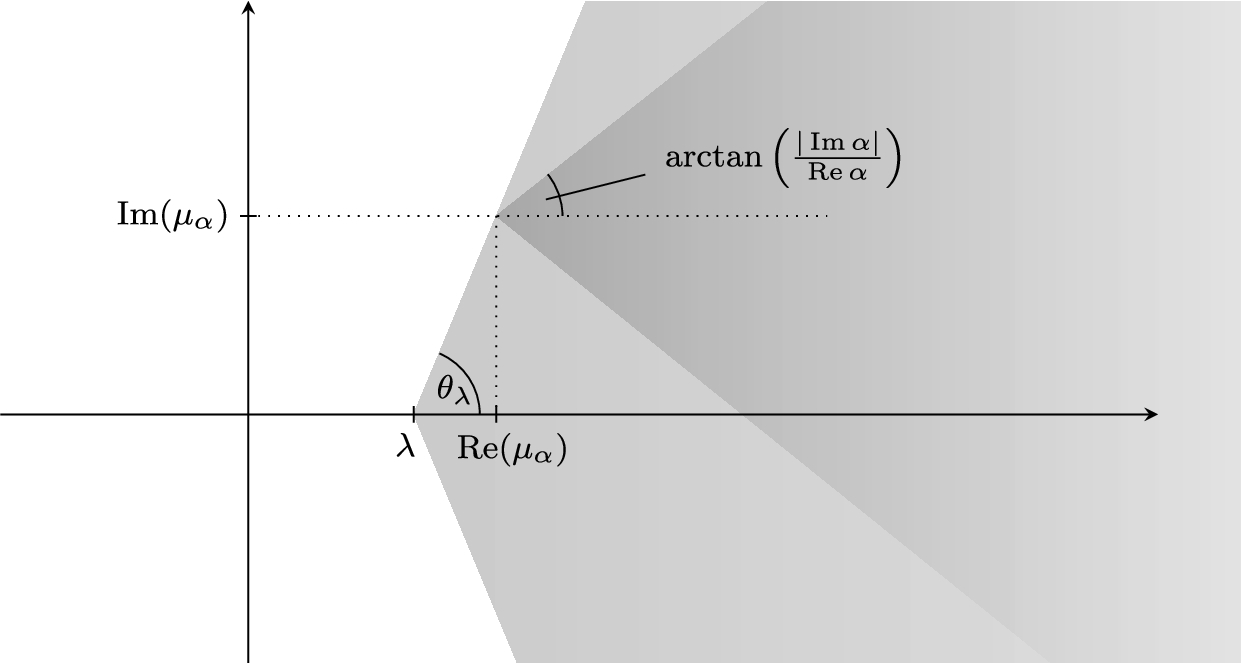\end{array}$ Recall from Section 1 that $μ_{α} = α S_{d} / 2^{d}$ and hence $| Im μ_{α} | / Re μ_{α} = | Im α | / Re α$ . Combining this with (7.1), we obtain (cf. Figure 2) $\begin{array}{l} | Im ⟨ (B^{α} - λ) u, u ⟩ | & ⩽ \frac{| Im α |}{Re α} (Re μ_{α} + Re α ‖ u ‖_{L^{2} (\partial Ω)}^{2}) \\ ⩽ \frac{| Im α |}{Re α} (Re ⟨ (B^{α} - λ) u, u ⟩ + λ) \\ ⩽ \frac{| Im α |}{Re α - \frac{λ}{2^{- d} S_{d}}} Re ⟨ (B^{α} - λ) u, u ⟩ . \end{array}$

Fig. 2.

The sector of decay and angle $θ_{λ}$ for $B^{α}$ .

Using standard generation theorems about analytic semigroups, the next statement follows.

Proposition 7.1.

The operator $- (B^{α} - λ)$ generates a bounded analytic semigroup in the sector $Σ_{\frac{π}{2} - θ_{λ}}$ , where $\begin{matrix} θ_{λ} = arctan (\frac{| Im α |}{Re α - \frac{λ}{2^{- d} S_{d}}}) . \end{matrix}$ Equivalently, $- B^{α}$ generates an analytic semigroup with $\begin{matrix} ‖ exp (- z B^{α}) ‖ ⩽ exp (- λ z) \forall z \in Σ_{\frac{π}{2} - θ_{λ}} . \end{matrix}$

Proof.

See [6, Ch. IX.1.6]. □

7.2. Decay of

e^{- t (A_{ε}^{α} - Id)}

In this section we denote $B_{ε}^{α} : = A_{ε}^{α} - Id$ . By calculations analogous to the above, we have $\begin{array}{l} | Im ⟨ B_{ε}^{α} u, u ⟩ | & ⩽ \frac{| Im α |}{Re α} Re ⟨ B_{ε}^{α} u, u ⟩, \end{array}$ that is, $B_{ε}^{α}$ is sectorial with sector $Σ_{θ_{0}}$ , where $θ_{0} = arctan (| Im α | / Re α)$ , and hence generates a bounded analytic semigroup in the sector $Σ_{\frac{π}{2} - θ_{0}}$ . In this subsection we improve this a priori result using spectral convergence. To this end, let $δ > 0$ and define the compact set $\begin{matrix} K_{δ} : = {x + i y : x \in [0, Re μ_{α}], y \in [- | Im μ_{α} |, | Im μ_{α} |]} . \end{matrix}$ Note that then $Σ_{θ_{0}} \cap {Re z ⩽ Re μ_{α} - δ} \subset K_{δ}$ . By [4, Th. III.2.3] one has $K_{δ} \subset ρ (B^{α})$ for every $δ > 0$ . Applying Corollary 3.3 we see that for every $δ > 0$ there exists a $ε_{0} > 0$ such that $K_{δ} \subset ρ (B_{ε}^{α})$ for all $ε < ε_{0}$ .

In particular we have shown that the resolvent norm $‖ {(B_{ε}^{α} - z)}^{- 1} ‖$ is bounded on $Σ_{θ_{0}} \cap {Re z ⩽ Re μ_{α} - δ}$ . By a trivial calculation analogous to the previous subsection this leads to the following statement.

Lemma 7.2.
For every $λ \in (0, Re μ_{α} - δ)$ one has $\begin{matrix} σ (B_{ε}^{α} - λ) \subset Σ_{θ_{λ}^{δ}}, θ_{λ}^{δ} = arctan (\frac{| Im μ_{α} |}{Re μ_{α} - λ - δ}) . \end{matrix}$

Furthermore, we obtain the following lemma.
Lemma 7.3.
For every $λ \in (0, Re μ_{α} - δ)$ one has $C ∖ Σ_{θ_{λ}^{δ}} \subset ρ (B_{ε}^{α} - λ)$ and there exists a $M = M (λ, δ) > 0$ such that $\begin{matrix} ‖ {(B_{ε}^{α} - λ - z)}^{- 1} ‖ ⩽ \frac{M}{| z |} \forall z \in C ∖ Σ_{θ_{λ}^{δ}} . \end{matrix}$
Proof.
This is obtained by combining Lemma 7.2 with the following two facts: $\begin{matrix} | Im ⟨ B_{ε}^{α} u, u ⟩ | ⩽ \frac{| Im α |}{Re α} Re ⟨ B_{ε}^{α} u, u ⟩, ‖ {(B_{ε}^{α} - z)}^{- 1} ‖ ⩽ C on K_{δ} . \end{matrix}$ □

By the theory of analytic semigroups (cf. [6, Ch. IX.1.6]), we immediately obtain the following corollary.
Corollary 7.4.
For all $λ \in (0, Re μ_{α} - δ)$ , the operator $B_{ε}^{α} - λ$ generates a bounded analytic semigroup in the sector $Σ_{\frac{π}{2} - θ_{λ}^{δ}}$ .

This yields the main result of this section, as follows. Theorem 7.5.
For every $δ > 0$ there exists $ε_{0} > 0$ such that for every $λ \in (0, Re μ - δ)$ there exists $M > 0$ such that $\begin{matrix} ‖ exp (- z B_{ε}^{α}) ‖ ⩽ M exp (- λ Re z) \forall z \in Σ_{θ_{λ}^{δ}}, ε \in (0, ε_{0}) . \end{matrix}$
Remark 7.6.
It is straightforward to repeat the above proof for the case of Dirichlet boundary conditions to obtain an analogous result for $‖ exp (- t (A^{D} - Id)) ‖$ . Here, the selfadjointness of $A^{D}$ allows us to choose the half-angle θ arbitrarily close to $π / 2$ .

8. Conclusion

We have shown norm-resolvent convergence in the classical perforated domain problem with Dirichlet boundary conditions which has the interesting implication of spectral convergence (Cor. 3.3). Some questions remain open and will be addressed in the future. While the norm $‖ J_{ε} A_{ε}^{- 1} - A^{- 1} J_{ε} ‖_{L (L^{2} (Ω_{ε}), L^{2} (Ω))}$ converges to 0, it is not clear from our method of proof how fast this happens. It would be desirable to obtain a precise convergence rate. In the case of Dirichlet boundary conditions a explicit convergence rate has been found by [10]. Another interesting question is whether in the case $Ω = R^{d}$ there exist gaps in the spectrum of $A_{ε}$ and how these depend on ε. The existence of spectral gaps has been confirmed in two dimensions [9], but to the authors’ knowledge the higher-dimensional case is still open.

Footnotes

Acknowledgements

KC is grateful for the financial support of the Engineering and Physical Sciences Research Council (UK): Grant EP/L018802/2 “Mathematical foundations of metamaterials: homogenisation, dissipation and operator theory”.

References

Brezis, Functional Analysis, Sobolev Spaces and Partial Differential Equations, Universitext, 2011 edn, Springer, 2010.

Cioranescu and

Murat, A strange term coming from nowhere, Progress in Nonlinear Differential Equations and Their Applications 31 (1997), 45–93.

DiBenedetto, Real Analysis, Birkhäuser Advanced Texts, Birkhäuser, Boston, 2002.

D.E.

Edmunds and

W.D.

Evans, Spectral Theory and Differential Operators, Oxford Mathematical Monographs, Oxford University Press, 1987.

Kaizu, The Robin problems on domains with many tiny holes, in: Proc. Japan Acad., Ser. A, Vol. 61, 1985.

Kato, Perturbation Theory for Linear Operators, Classics in Mathematics, Springer, 1995, reprint of the corr. 2nd edition.

V.A.

Marchenko and

E.Y.

Khruslov, Boundary-value problems with fine-grained boundary [in Russian], Mat. Sb. (N. S.) 65(107) (1964), 458–472.

Mugnolo,

Nittka and

Post, Norm convergence of sectorial operators on varying Hilbert spaces, Operators and Matrices 7(4) (2013), 955–995. doi:10.7153/oam-07-54.

S.A.

Nazarov,

Ruotsalainen and

Taskinen, Spectral gaps in the Dirichlet and Neumann problem on the plane perforated by a double-periodic family of circular holes, Journal of Mathematical Sciences 181(2) (2012). doi:10.1007/s10958-012-0681-y.

10.

Post and

Khrabustovskyi, Operator estimates for the crushed ice problem, ArXiv e-prints, arXiv:1710.03080.

11.

Rauch and

Taylor, Potential and scattering theory on wildly perturbed domains, J. Funct. Anal. 18 (1975), 27–59. doi:10.1016/0022-1236(75)90028-2.

12.

R.T.

Rockafellar and

R.J.-B.

Wets, Variational Analysis, Grundlehren der Mathematischen Wissenschaften [Fundamental Principles of Mathematical Sciences], Vol. 317, Springer-Verlag, Berlin, 1998.

13.

A.E.

Taylor and

D.C.

Lay, Introduction to Functional Analysis, Wiley, 1980.