Sage Journals: Discover world-class research

Abstract

Educational researchers often report effect sizes in standard deviation units (SD), but SD effects are hard to interpret. Effects are easier to interpret in percentile points, but converting SDs to percentile points involves a calculation that is not transparent to educational stakeholders. We show that if the outcome variable is normally distributed, we can approximate the percentile-point effect simply by multiplying the SD effect by 37 (or, equivalently, dividing the SD effect by 0.027). For students in the middle three-fifths of a normal distribution, this rule of thumb is always accurate to within 1.6 percentile points for effect sizes of up to 0.8 SD. Two examples show that the rule can be just as accurate for empirical effects from real studies. Applying the rule to empirical benchmarks, we find that the least effective third of educational interventions raise scores by 0 to 2 percentile points; the middle third raise scores by 2 to 7 percentile points; and the most effective third raise scores by more than 7 percentile points.

Keywords

communication decision making educational policy effect size

Educational researchers often report effect sizes in standard deviations (SD). For example, a study might report that treatment raised some students’ test scores by 0.2 SD—meaning that those students scored 0.2 SD higher, on average, than they would have without treatment.

Yet effects reported in SD units are unintuitive. When told that a program raised test scores by 0.2 SD, a nonprofit leader or principal will often ask, “Is that good or bad?” Different researchers answer this question differently. Some describe effects of nearly 0.2 SD as “quite large” (e.g., Kane & Staiger, 2008), while others describe them as “trivial to small” (e.g., Cheng et al., 2019).

Not only do researchers disagree on which SD effects are large or small, many researchers also have biased and unreliable intuitions about what effects expressed in SD units actually look like. When asked to illustrate an effect size of 0.2 SD, most researchers produce a misleading graph that at least doubles the requested effect, showing two normal distributions that are separated by 0.4 SD or more (Schuetze & Yan, 2023). Conversely, when shown two normal distributions that are actually separated by 0.2 SD, most researchers underestimate the illustrated effect, guessing that it is 0.05 SD or less. Impressions of visually presented effect sizes vary dramatically across researchers, suggesting that we do not share a common or realistic understanding of what SD effects really represent (Schuetze & Yan, 2023).

One way to describe effects more intuitively is to express them in percentile points. Because standardized test scores are commonly reported as percentiles, many students, parents, teachers, and administrators understand that scoring at, say, the 50th percentile means scoring higher than half of students. They can also appreciate that improving a score by 10 percentile points—say from the 50th to the 60th percentile—means scoring higher than an additional 10% of students. So compared to SD effects, percentile point effects are relatively clear and accessible, not just to researchers but also to education stakeholders at all levels. The What Works Clearinghouse (2022) calls percentile point effects an “improvement index” and argues that they can “help readers judge the practical importance of the magnitude of intervention effects.”

It is possible to calculate percentile point effects directly, for example, by comparing the median percentile rank of treated and control students at the end of a study. But few studies do this, and reporting effects in SD units remains the norm. So people who communicate or consume the results of educational research need a quick, convenient, and transparent way to translate reported SD effects into equivalent percentile point effects.

In carrying out the translation, it is common to assume that the outcome variable—often a test score—is normally distributed. For a student who would score at the median of a normal distribution without treatment, an effect of 0.2 SD would raise their score by 8 percentile points—from the 50th percentile to the 58th. Translating an effect from 0.2 SD to 8 percentile points can convert a frustrating and abstract technical conversation about what an effect of 0.2 SD really means into a concrete policy conversation about whether an improvement of 8 percentile points is worth the intervention’s cost in time, trouble, or money.

There are two concerns that deter researchers from converting effects to percentile points as often as we might like. First, the calculation is widely thought to require using the cumulative standard normal distribution. The calculation is not difficult for someone with a little statistical training and a spreadsheet, but it is not a calculation that many of us can do in our heads, and it is far from transparent to an education leader with limited statistical training. In fact, explaining the cumulative normal distribution to someone who is unfamiliar with it is every bit as hard as explaining an SD effect.

The second concern is that conversion from SDs to percentile points sometimes depends on where the student lies in the distribution. For a student who would score at the median without treatment, an effect of 0.20 SD will raise their percentile rank by 8 points (from the 50th percentile to the 58th). But for a student who would score at the 10th percentile without treatment, an effect of 0.20 SD will only raise their percentile rank by half as much—by 4 percentile points (from the 10th percentile to the 14th).

While both these concerns are valid, they only apply to unusually large effect sizes and students in the tails of the distribution. The following rule of thumb works surprisingly well for most students and the vast majority of effects reported in educational research:

To convert an SD effect to approximate percentile points, simply multiply the SD effect by 37.

For example, an effect of 0.1 SD is equivalent to raising affected students’ scores by 3.7 (or approximately 4) percentile points. Since 37 is the reciprocal of 0.027, the following rule is equivalent:

To convert an SD effect to approximate percentile points, simply divide the SD effect by 0.027.

This version of the rule is more transparent in some settings. For example, it is immediately clear that an effect size of 0.27 SD is equivalent to raising scores by 10 percentile points.

Unlike calculations involving the cumulative standard normal distribution, multiplying by 37 is a transparent calculation that many of us can approximate in our heads while reading a report, giving a presentation, or discussing results in a meeting. We do not need to consult a table or spreadsheet, and we can explain the calculation to stakeholders who have limited statistical training. Yet for most students and the vast majority of effect sizes, multiplying by 37 usually comes within 1 percentile point of the result obtained by using the cumulative normal distribution.

The calculation can also be reversed. For example, suppose you are planning a trial of a novel intervention. To clarify stakeholders’ hopes, or calculate the sample size required to detect the effect, you would like a practitioner to tell you how large an effect they expect, or how small an effect would disappoint them. The practitioner may have trouble expressing their hopes in SD units, but they may more readily express themselves in percentile points. To translate their percentile point guess into SD units, you can simply divide it by 37.

In the rest of this article, we’ll demonstrate the multiply-by-37 rule and explain its rationale, uses, and limitations. All data and code used in this article are available in the online Supplemental Materials, and at https://osf.io/jf534/

Using the Rule in Data From a Normal Distribution

To start, let’s assume that the outcome variable has a normal distribution. Then, we can convert an effect from SD units to percentile points in two different ways:

an exact formula (given later) which uses the cumulative standard normal distribution, versus

an approximation, which simply multiplies the SD effect by 37.

The top of Figure 1 compares these approaches for a student who, if untreated, would score at the median. For such a student, the two approaches agree closely. For any effect size up to 0.8 SD—that is, for over 90% of effects reported in educational research (Kraft, 2020)—approximation of multiplying the SD effect by 37 comes within less than 1 percentile point of the exact answer obtained by using the cumulative normal distribution. For example, an effect of 0.8 SD translates to 28.8 percentile point if we use the cumulative normal distribution, or 29.6 percentile point if we multiply by 37. The approximation error is just 0.8 percentile points.

Figure 1.

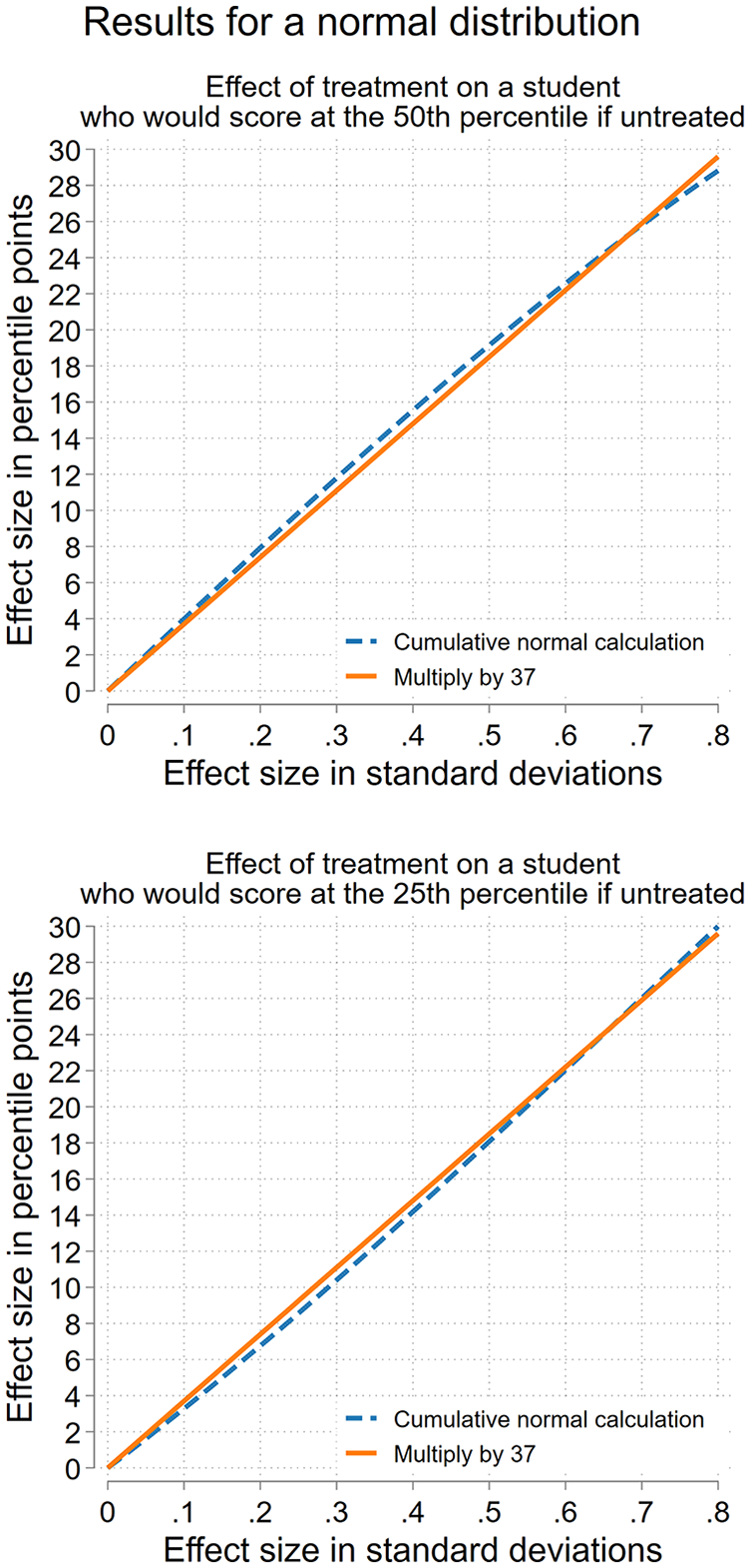
Theoretical accuracy of the multiply-by-37 rule for translating effect sizes from standard deviations to percentile points in a normal distribution.

Percentile point effects are often reported as though they were only valid for students near the 50th percentile. But as the bottom of Figure 1 shows, multiplying by 37 works just as well for a student who, if untreated, would score at the 25th percentile of a normal distribution. For such a student, an effect of 0.80 SD translates to 30.0 percentile point if we use the cumulative normal distribution, or 29.6 percentile point if we multiply by 37—an approximation error of just 0.4 percentile points. More generally, for a student who if untreated would score at the 25th percentile of a normal distribution, multiplying by 37 comes within 1 percentile point of the exact answer (obtained using the cumulative normal distribution) for any effect size of between 0 and 0.8 SD (and even larger).

In general, if the outcome is normally distributed, multiplying by 37 usually comes within 1 percentile point of the exact answer—and always comes within 1.6 percentile points—for any student whose score stays approximately in the middle three-fifths of the distribution.

Can the Rule Work in Real Data?

Figure 2 shows that multiplying by 37 can also work well for effects from real empirical studies. To check this, we used results from two studies that reported effects in both SDs and percentile points:

Figure 2.

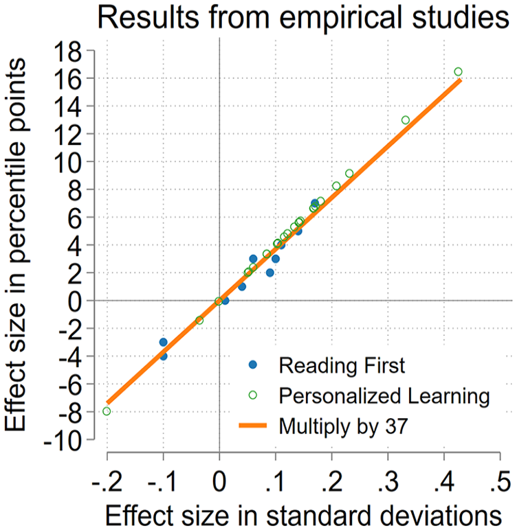
Empirical accuracy of the multiply-by-37 rule for converting effects observed in empirical studies from standard deviations to percentile points.

One study was a randomized controlled trial of a “personalized learning” intervention. The trial report estimated 24 effects of personalized learning—one effect for each of two subjects (reading, math) in each of 12 grades (kindergarten through 11th; Baird & Pane, 2019; Pane et al., 2017).

The other study was a regression discontinuity evaluation of the federally funded Reading First program (Gamse et al., 2008). The study report estimated 11 effects of Reading First; each estimate represented the program’s effect on some skill (reading comprehension or the ability to decode letters into sound) at some grade level (1st, 2nd, or 3rd). Effects were also broken out by years of exposure (1, 2, 3, or all exposures together) and by when schools received Reading First funding (early, late, or all schools together).

Among 35 effects ranging from −0.20 SD to +0.43 SD (or −8 to +16 percentile points), multiplying the reported SD effect by 37 came within 1 point of the reported percentile point effect in every case but one.

This example shows that multiplying by 37 can be useful even if the outcome variable does not have a perfectly normal distribution. In the personalized learning study, the outcomes were math and reading scores from the Measures of Academic Progress (MAP) test published by NWEA. The distribution of MAP scores can deviate noticeably from normality in the left tail.¹ In the Reading First Impact Study, one outcome was reading comprehension scores from the Stanford Achievement Test, 10th edition (SAT10), whose distribution can be bimodal, platykurtic, skewed left, or skewed right (Shanley et al., 2019). Another outcome was decoding scores from the Test of Silent Word Reading Fluency, which counts the words that a student can read in 3 minutes; note that counts are often skewed to the right.

The empirical accuracy of multiplying these study estimates by 37 is also encouraging because each study calculated the percentile point effect somewhat differently. Neither study assumed that scores were normally distributed. Instead, in the Reading First Impact Study, the mean test scores of the treatment and control groups were converted to corresponding percentiles in a national reference distribution and then the control percentile was subtracted from the treatment percentile. Mean scores in the control condition were between the 33rd and 46th percentiles, showing again that percentile gains (and the multiply-by-37 approximation) are not valid only at the median. Both the treatment and control percentiles were rounded to the nearest whole number before subtracting, so the estimated difference suffers from rounding error and may differ by 1 percentile point from the true difference; this may explain some slight discrepancies between the reported percentile effects and the approximation of multiplying by 37.

The personalized learning study estimated percentile point effects in a more complicated way—estimating the distribution of the control group’s scores and then calculating the percentile that would be achieved if one added the treatment effect to the control median. The investigators noted that they estimated the control distribution in a nonparametric fashion that did not assume normality but “allow[ed] the distribution of scores to take any shape, such as skewed, bimodal, or highly kurtotic” (Baird & Pane, 2019, p. 223).

Despite these encouraging results, we would not claim that multiplying by 37 works well for every educational outcome. Surely, someone could find a highly non-normal distribution where it worked poorly—but then the usual cumulative normal calculation would work poorly as well! Our point is not that multiplying by 37 is always accurate, but that when the cumulative normal calculation is accurate, multiplying by 37 usually works practically as well.

Benchmarks for Percentile Point Effects

Although converting SD effects to percentile points makes them more interpretable, it can still be helpful to interpret percentile point effects with respect to some benchmark.

Table 1 uses the multiply-by-37 rule to convert benchmarks for effect size from SD units to percentile points. For example, Kraft (2020) derived empirical benchmarks from an inventory of rigorous studies of educational interventions. Converted from SDs to percentile points, Kraft’s benchmarks suggest that the least effective third of interventions raise most students’ scores by 0 to 2 percentile points, the middle third raise scores by 2 to 7 percentile points, and the most effective third raise scores by more than 7 percentile points.

Table 1

Benchmarks for Effect Size

	Effect size
Source	Units	Small	Medium	Large
Cohen (1970)	Standard deviations	0.2	0.5	0.8
	Percentile points	7	19	30
Kraft (2020)	Standard deviations	0.05	0.05 to 0.2	0.2
	Percentile points	Less than 2	2 to 7	More than 7

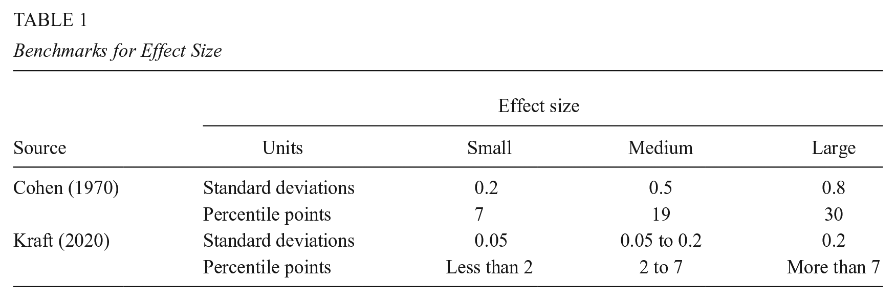
Kraft’s benchmarks contrast with Cohen’s (1970) older benchmarks, which when converted to percentile points suggested that “small” effects raised most scores by approximately 7 percentile points, “medium” effects raised scores by approximately 19 percentile points, and “large” effects raised scores by approximately 30 percentile points. Cohen’s benchmarks were “somewhat arbitrary” (Cohen, 1962) and based on his experience with laboratory experiments in psychology. Cohen (1970) cautioned that they should not be generalized to other fields, but they have been widely used in education, where they now seem quite optimistic. According to Kraft’s inventory, 70% of education effects would be “small” by Cohen’s standards, and only 5% of effects (less than 1% in large studies) would be “large” by Cohen’s standards (Kraft, 2020, tbl. 1).²

Why Does It Work?

Figure 3 helps to illustrate why multiplying by 37 works for a normally distributed outcome. We will explain it in three different ways, starting with a simple explanation suitable for someone with limited exposure to statistics, and finishing with a more sophisticated explanation that uses a little calculus and optimization. We are brief in the article but provide more detail in the Supplementary Appendix in the online version of the journal.

Figure 3.

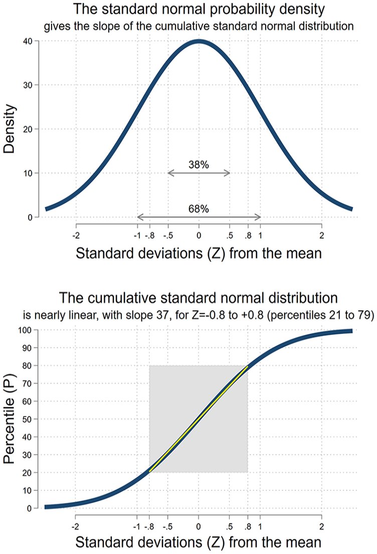
In a normal distribution, 38 percent of the area is in the 1 SD range between 0.5 SD below the mean to 0.5 SD above. 68 percent is in the 2 SD range between 1 SD below the mean and 1 SD above.

Explanation Using the Bell Curve

The top of Figure 3 shows the standard normal probability density function (PDF)—the familiar bell curve taught in practically every introductory statistics course. A familiar fact about the normal distribution, also taught in practically every course, is that 68% of the probability lies within 1 SD of the mean. So an effect that raises a student’s score from 1 SD below to 1 SD above the mean would raise their score by 68 percentile points. In this example, a 2 SD effect is equivalent to 68 percentile points, suggesting a rule that multiplies the SD effect by 34—not too far from 37.

Another fact about the normal distribution, not taught as often, is that 38% of the probability lies within half a SD of the mean. So an effect that raises a student’s score from 0.5 SD below to 0.5 SD above the mean would raise their score by 38 percentile points. In this example, a 1 SD effect is equivalent to 38 percentile points, suggesting a rule that multiplies the SD effect by 38—again not too far from 37.

In general, the best multiplier depends on where a student starts in the distribution and how much the intervention increases or decreases their score. But for students who stay in the middle three-fifths of the distribution, multipliers between 34 and 40 work reasonably well, and a multiplier of 37 works best on average.

Explanation Using the Cumulative Normal Distribution

The next two sections are more technical and some readers may wish to skip to the conclusion. Figure 3 shows the standard normal cumulative distribution function (CDF), which represents the relationship between a student’s percentile rank P and how many standard deviations Z they are from the mean of a normal distribution. The standard normal CDF is often represented by the Greek letter $Φ$ :³

P = Φ (Z) .

For example, a student who is 0 standard deviations from the mean is at the 50th percentile ( $Φ (0) = 50$ ), a student who is Z = 0.8 standard deviations above the mean is at the 79th percentile ( $Φ (0.8) = 79$ ), and a student who is Z = 0.8 standard deviations below the mean is at the 21st percentile ( $Φ (- 0.8) = 21$ ).

Over the full range of the distribution, the CDF has an S shape, but between the P = 21st and 79th percentiles—that is, between Z = 0.8 SD above and Z = −0.8 SD below the mean—the CDF is approximately linear with an intercept of 50 and a slope not too far from 37:

\hat{P} = \hat{Φ} (Z) = 50 + 37 Z .

The linear approximation $\hat{P}$ comes within 0.8 percentile points of the true value of P for every value of Z from −0.8 to 0.8.

This means that multiplying by 37 translates an SD effect into an approximate percentile point effect, provided the student stays between the 21st and 79th percentile. To see that explicitly, notice that the SD effect on an individual student ( $Δ Z$ ) is the difference between how many standard deviations from the mean they would score under treatment (Z_t) versus how many standard deviations from the mean they would score under the control (Z_c):

Δ Z = Z_{t} - Z_{c} .

Likewise, the percentile point effect on an individual student ( $Δ P$ ) is the difference between the student’s percentile rank under treatment (Z_t) and their percentile rank under control (Z_c):

Δ P = P_{t} - P_{c} .

Over the full range of the normal distribution, the exact relationship between $Δ P$ and $Δ Z$ is not linear:

\begin{array}{l} Δ P = P_{t} - P_{c} \\ = Φ (Z_{t}) - Φ (Z_{c}) \end{array}

(exact formula).

But in the range where $Φ (Z)$ can be approximated by 50+37 P, the percentile point effect can be approximated by

\begin{array}{l} Δ \hat{P} = \hat{Φ} (Z_{t}) - \hat{Φ} (Z_{c}) \\ \approx (50 + 37 Z_{t}) - (50 + 37 Z_{c}) \\ = 37 Δ Z \end{array}

(approximation).

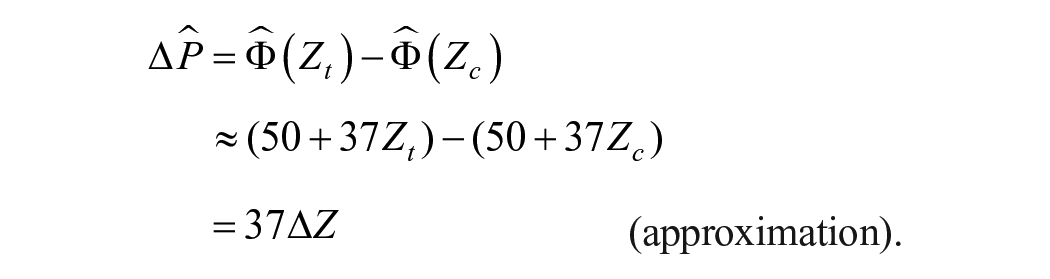
That is, multiplying the SD effect by 37 can approximate the percentile point effect.

Explanation Relating the Bell Curve to the Cumulative Distribution Function

The previous explanations are compatible, because the PDF in the first explanation is related to the CDF in the second. Specifically, the PDF is the derivative or slope of the CDF, as students are taught in every mathematical statistics course (e.g., Hogg et al., 2012).⁴ Knowing this, you can look at the PDF (top of Figure 3) to get the slope of the CDF (bottom of Figure 3) at each value of Z (SDs from the mean).

Specifically, at the mean (Z = 0), the slope of the CDF is 40; at 0.4 SD above or below the mean (Z = 0.4 or −0.4), the slope is 37; and at 0.8 SD above or below the mean (Z = 0.8 or −0.8), the slope is 29. This is why our discussion of the bell curve found that larger multipliers were appropriate for students closer to the mean. Although the optimal slope is not exactly 37 through the whole range from Z = +0.8 to −0.8, it is close enough for 37 to be a good approximation for students who stay within this range.

When Does Multiplying by 37 Work?

We have stated that multiplying by 37 works for students who “stay” between the 21st and 79th percentile (or, equivalently, between Z = +0.8 and −0.8 SDs from the mean). We should be explicit about what we mean by “stay.” Multiplying the SD effect by 37 works for students who would score between the 21st and 79th percentile without treatment, and would still score between the 21st and 79th percentile if they were treated.

If treatment takes a student outside of that range, or if they would score outside that range if they were untreated, then multiplying the SD effect by 37 does not work as well, because the student will have strayed outside the range where the relationship between percentiles and SDs is approximately linear. More specifically, if the treated or untreated score is in the top or bottom 20% of a normal distribution, then multiplying the SD effect by 37 will always overestimate the percentile point effect.

But knowing when we are overestimating an effect is useful, too, because it means that, in the tails, we can treat multiplying by 37 as an upper bound. It can be useful to place an upper bound on effect size, particularly if the effect is small. For example, if an SD effect is 0.05 SD, we can say that it is only 2 percentile points for students in the middle three-fifths of the distribution—and even less for students in the tails.

We tailored the multiply-by-37 rule to work for normally distributed outcomes, but Figure 2 showed that it can also work reasonably well for real test scores, which do not have a perfectly normal distribution. While we would not claim that multiplying by 37 works for any data regardless of how it is distributed, we should point out that, since the rule is only meant to in the middle three-fifths of the distribution, non-normality in tails may not matter as much. For example, histograms shared with us by the publisher of the MAP tests (NWEA) suggest that MAP scores depart from normality primarily in the bottom 20% of the distribution. This may not have affected results from the Reading First Impact Study (Figure 2), which estimated the effect of Reading First on the MAP scores of students who would score in the 33rd to 50th percentiles if untreated.

Why 37?

Multiplying by 37 is just an approximation, and other multipliers are certainly possible. Any multiplier between 35 and 40 would give fairly similar estimates. A case can be made for multiplying by 40 because it is an easier mental calculation and gives very serviceable estimates, especially for small effects near the median.

That said, multiplying by 37 is optimal in the sense that it ensures the approximation error is never larger than 1.6 percentile points (and usually smaller than 1 percentile point) for students who stay between the 21st and 79th percentile of a normal distribution.

A different multiplier would be optimal if we focused on a different range of the normal distribution or tried to minimize a different function of the approximation error (such as the mean squared error). But the range between the 21st and 79th percentile seems to be the widest range over which any multiplier can work well, and it seemed desirable to minimize the largest error that can occur, rather than just ensuring that, say, squared errors are small on average.

The Supplementary Appendix in the online version of the journal gives more detail on the derivation and properties of multiplying by 37.

Other Ways to Interpret Effect Sizes

Although it does put effects on a more interpretable scale, converting effects from SDs to percentile points does not eliminate the need to interpret effect sizes in other ways. For example, as we remarked earlier, it can be useful to compare an effect to empirical benchmarks, and judge whether the effect is small (0–2 percentile points), medium (2–7), or large (more than 7) when compared to alternatives.

It can also be helpful to compare the effect of an intervention to its cost. As several authors have pointed out, if two interventions achieve similar effects, we should prefer the intervention with lower cost; likewise if two interventions have similar costs, we should prefer the intervention with the larger effect (Kraft, 2020; Levin et al., 2017). However, if interventions differ in both cost and effect, then comparison is more difficult. For example, suppose one intervention produces an effect of 0.06 SD (2 percentile points) at a cost of $100 per student, while an alternative can produce an effect 10 times larger (0.6 SD, 22 percentile points) at a cost that is 20 times higher ($2,000 per student). Measured in SDs or percentile points per dollar, the first intervention appears twice as cost-effective (Harris, 2009), but it only raises scores by 2 percentile points. The 22 percentile point improvement of the second intervention could be worth paying for, even if the cost per percentile point is twice as high.

Another popular option is to translate the effect into months or years or learning. This attractive metric is easy to apply in longitudinal studies where the benefit to the treatment group can be compared to the amount learned by the control group. But it is more problematic to compare the effect of an intervention to the amount learned by different students in a different study. The challenge is that learning rates are not constant but vary by age, subject, test, and other factors. Age is the most important factor; in general, young children gain reading and math skills much faster than older children, so that an effect of 0.2 SD is equivalent to about a month of learning in kindergarten but a year of learning in ninth grade (Bloom et al., 2008). When grade is held constant, annual gains still vary across tests; ninth grade reading gains, for example, can be as large as 0.32 SD or as small as 0.04 SD, depending on what test is used to measure them (Bloom et al., 2008). Annual gains can be averaged across different tests, but the multi-test average may not be a suitable benchmark for an effect obtained on one test in particular. On some tests, but not others, annual gains are different over 12 months than over a 9-month academic year that excludes summer vacation (Workman et al., 2023). Annual gains vary across times and places (Matheny et al., 2023). They vary across subjects (Bloom et al., 2008). For some subjects, such as Latin, probability, or cartography, there may be no benchmarks for annual gains at all. In short, while it can be helpful to keep annual gains in mind as a rough comparison, converting effects into months or years of learning is often challenging to do with much precision. The challenge is fundamental, and switching from SDs to percentile points does not solve it.

Another option is to compare an effect to a gap in test scores between advantaged and disadvantaged children. This comparison can be appropriate in some settings, for example, in a study that asked whether certain charter schools shrank the gap in reading and math scores between Black children in Harlem and White children elsewhere in New York City (Dobbie & Fryer, 2011). But the comparison is not always pertinent and, if used habitually, can give the misleading and undesirable impression that score gaps are so constant and immutable that they can be engraved on a ruler (Quinn, 2020). In fact, score gaps between groups of children vary substantially across places, times, subjects, tests, grade levels, and the group characteristics used (e.g., family income, parental education, school-level poverty, or race and ethnicity; Reardon et al., 2019; U.S. Department of Education, 2023). The variable nature of score gaps can make it difficult to treat them as a fixed ruler to measure effect size.

Conclusion

Careful educational researchers take pains to estimate treatment effects precisely and without bias. Yet we then describe those effects in SD units that many practitioners find unintelligible, and even trained researchers interpret in biased and inconsistent ways. Translating effects into percentile points puts effects on a shared and intelligible scale—and it can usually be accomplished simply by multiplying the SD effect by 37 (or dividing by 0.027).

Even on an intelligible percentile point scale, educators and scholars may have different ideas about whether an effect is large enough to matter. Some may think that any effect smaller than 10 percentile points (0.27 SD) is negligible, while others may argue that even effects of 2 percentile points (0.05 SD) can be important in some settings. Translating effects into percentile points will not end all debate. But it is a good start to a conversation.

Supplemental Material

sj-docx-1-epa-10.3102_01623737241239677 – Supplemental material for Multiply by 37 (or Divide by 0.027): A Surprisingly Accurate Rule of Thumb for Converting Effect Sizes From Standard Deviations to Percentile Points

Supplemental material, sj-docx-1-epa-10.3102_01623737241239677 for Multiply by 37 (or Divide by 0.027): A Surprisingly Accurate Rule of Thumb for Converting Effect Sizes From Standard Deviations to Percentile Points by Paul von Hippel in Educational Evaluation and Policy Analysis

Footnotes

Acknowledgements

I thank Matthew Baird and John Pane for sharing estimates from their 2019 Educational Researcher article, “Translating standardized effects of education programs into more interpretable metrics.”

Declaration of Conflicting Interests

The author(s) declared no potential conflicts of interest with respect to the research, authorship, and/or publication of this article.

Funding

The author(s) received no financial support for the research, authorship, and/or publication of this article.

Supplemental Material

Data, code, and a PDF containing additional calculations and figures are available in the online Supplemental Materials. Data and code are also available at the Open Science Framework ().

Notes

Author

PAUL VON HIPPEL, PhD, is a professor and associate dean for research at the LBJ School of Public Affairs, The University of Texas at Austin. His current research focuses on translating the science of learning into policy.

References

Baird

M. D.

Pane

J. F.

(2019). Translating standardized effects of education programs into more interpretable metrics. Educational Researcher, 48(4), 217–228. https://doi.org/10.3102/0013189X19848729

Bloom

H. S.

Hill

C. J.

Black

A. B.

Lipsey

M. W.

(2008). Performance trajectories and performance gaps as achievement effect-size benchmarks for educational interventions. Journal of Research on Educational Effectiveness, 1(4), 289–328. https://doi.org/10.1080/19345740802400072

Cheng

Ritzhaupt

A. D.

Antonenko

(2019). Effects of the flipped classroom instructional strategy on students’ learning outcomes: A meta-analysis. Educational Technology Research and Development, 67(4), 793–824. https://doi.org/10.1007/s11423-018-9633-7

Cohen

(1962). The statistical power of abnormal-social psychological research: A review. The Journal of Abnormal and Social Psychology, 65(3), 145–153. https://doi.org/10.1037/h0045186

Cohen

(1970). Approximate power and sample size determination for common one-sample and two-sample hypothesis tests. Educational and Psychological Measurement, 30(4), 811–831. https://doi.org/10.1177/001316447003000404

Dobbie

Fryer

R. G.

(2011). Are high-quality schools enough to increase achievement among the poor? Evidence from the Harlem children’s zone. American Economic Journal: Applied Economics, 3(3), 158–187.

Gamse

B. C.

Jacob

R. T.

Horst

Boulay

Unlu

(2008). Reading first impact study. Final report (NCEE 2009-4038). National Center for Education Evaluation and Regional Assistance. https://eric.ed.gov/?id=ED503344

Harris

D. N.

(2009). Toward policy-relevant benchmarks for interpreting effect sizes: Combining effects with costs. Educational Evaluation and Policy Analysis, 31(1), 3–29. https://doi.org/10.3102/0162373708327524

Hogg

McKean

Craig

(2012). Introduction to mathematical statistics (7th ed.). Pearson.

10.

Kane

Staiger

D. O.

(2008, February). Estimating teacher impacts on student achievement: An experimental evaluation (Working Paper 14607). National Bureau of Economic Research.

11.

Kraft

M. A.

(2020). Interpreting effect sizes of education interventions. Educational Researcher, 49(4), 241–253. https://doi.org/10.3102/0013189X20912798

12.

Levin

H. M.

McEwan

P. J.

Belfield

Bowden

A. B.

Shand

(2017). Economic evaluation in education: Cost-effectiveness and benefit-cost analysis. Sage.

13.

Matheny

K. T.

Thompson

M. E.

Townley-Flores

reardon

s. f.

(2023). Uneven progress: Recent trends in academic performance among U.S. school districts. American Educational Research Journal, 60(3), 447–485. https://doi.org/10.3102/00028312221134769

14.

Pane

J. F.

Steiner

E. D.

Baird

M. D.

Hamilton

L. S.

Pane

J. D.

(2017). Informing progress: Insights on personalized learning implementation and effects. RAND Corporation. https://www.rand.org/pubs/research_reports/RR2042.html

15.

Quinn

D. M.

(2020). Experimental effects of “achievement gap” news reporting on viewers’ racial stereotypes, inequality explanations, and inequality prioritization. Educational Researcher, 49(7), 482–492. https://doi.org/10.3102/0013189X20932469

16.

Reardon

S. F.

Kalogrides

Shores

(2019). The geography of racial/ethnic test score gaps. American Journal of Sociology, 124(4), 1164–1221. https://doi.org/10.1086/700678

17.

Schuetze

B. A.

Yan

V. X.

(2023). Psychology faculty overestimate the magnitude of Cohen’s d effect sizes by half a standard deviation. Collabra: Psychology, 9(1), 74020. https://doi.org/10.1525/collabra.74020

18.

Shanley

Clarke

Anderson

D. A.

Turtura

Doabler

C. T.

Kurtz-Nelson

Fien

(2019). Exploring the utility of assessing early mathematics intervention response via embedded assessment. School Psychology, 34(5), 541–554. https://doi.org/10.1037/spq0000326

19.

U.S. Department of Education. (2023). NAEP dashboards—Achievement gaps. https://www.nationsreportcard.gov/dashboards/achievement_gaps.aspx

20.

What Works Clearinghouse. (2022). WWC version 5.0 procedures and standards handbook (WWC 2022008REV). U.S. Department of Education. https://ies.ed.gov/ncee/wwc/handbooks

21.

Workman

von Hippel

P. T.

Merry

(2023). Findings on summer learning loss often fail to replicate, even in recent data. Sociological Science, 10, 251–285.

Supplementary Material

Please find the following supplemental material available below.

For Open Access articles published under a Creative Commons License, all supplemental material carries the same license as the article it is associated with.

For non-Open Access articles published, all supplemental material carries a non-exclusive license, and permission requests for re-use of supplemental material or any part of supplemental material shall be sent directly to the copyright owner as specified in the copyright notice associated with the article.

0.00 MB

0.33 MB