
Abstract
This study investigates how individual states raise revenue to pay for elementary-secondary education spending following school finance reforms (SFRs). We identify states that increased and sustained education expenditures after reform, search for legislative statutes that appropriated more education spending, and assess how policymakers funded the SFRs. Our results show that state legislatures increase investments in education by increasing tax revenue streams, such as sales and excise taxes, and by taking over property tax collections. Considering these results, we discuss that increased state investment in education should be accompanied by a policy mechanism to distribute state aid equitably to districts. Moreover, policymakers should consider local voters’ preferences when implementing SFR policies, as tax increases may reduce local fiscal effort for education.
School finance reforms (SFRs) are typically defined as state-level education reforms resulting from court rulings or legislative statutes. Many of these reforms have induced states to either revise school funding formulas to provide equitable funding to school districts, increase state funding for elementary-secondary public education, or both (Jackson, 2020; Lafortune et al., 2018; Shores et al., 2023).
As research demonstrates, SFRs, on average, have led to increased education spending in public school districts across the United States, particularly among districts serving economically disadvantaged students (Lafortune et al., 2018; Liscow, 2018; Shores et al., 2023; Sims, 2011). This additional money matters for student outcomes (Jackson, 2020). Spending increases induced by SFRs have led to improvements in test scores (Lafortune et al., 2018); graduation rates (Candelaria & Shores, 2019); and adult outcomes, such as lower poverty incidence (Jackson et al., 2016) and upward intergenerational income mobility (Biasi, 2023).
The primary driver of increased district spending after an SFR is the expansion of state-level expenditures for elementary-secondary education (Card & Payne, 2002; Lafortune et al., 2018; Liscow, 2018; Shores et al., 2023). When state governments spend more on education, local school districts—the beneficiaries of state elementary-secondary education expenditures—receive these funds as state aid revenues. As a response to this increased state aid, school districts typically spend more on education, a phenomenon known as the flypaper effect (Card & Payne, 2002; Shores et al., 2023). Of course, other district-level revenue accounts—federal and local revenues—might also induce more district spending after an SFR; however, there is no evidence that these funds increase, on average, after reform (Lafortune et al., 2018; Shores et al., 2023).
Although state governments play an important role in increasing district spending, existing research does not systematically document and evaluate how individual states pay for SFRs. National-level studies find that state governments fund SFRs by raising taxes (Liscow, 2018) and not by reducing non-education-related state expenditures (Baicker & Gordon, 2006; Lafortune et al., 2018; Liscow, 2018; Murray et al., 1998). However, because these national studies leverage the differential timing of SFRs across states, they do not address state-specific heterogeneity. For example, it is not clear what types of taxes states choose to increase. Among state-level case studies that evaluate SFRs, some descriptively document how states pay for SFRs in a background section, while others estimate how they pay in an analysis section. Different methodologies across these state-specific studies make it difficult to have a benchmark for comparison across the states. For policymakers, the lack of standardized reporting across state-specific studies, along with national studies that do not document unique state actions, masks a feasible set of funding options for SFRs.
In this article, we seek to understand how state governments pay for increased state expenditures for elementary-secondary education. Addressing this question, however, comes with a challenge: Not all documented SFRs increase state expenditures for education (Shores et al., 2023). One explanation for this lack of state investment could be legislative postponement in the allocation of funds; some legislatures take years to adequately appropriate funds after an SFR (Candelaria et al., 2022; Sun et al., 2024). Alternatively, state legislatures might opt to redistribute funds from low-poverty to high-poverty districts without increasing funding. This scenario could happen if a state government assumes full funding control from local governments but does not have the fiscal capacity to increase state expenditures on education (Manwaring & Sheffrin, 1997; Silva & Sonstelie, 1995).
To ensure we can address our core question, we first identify a purposive case-study analytic sample by selecting states that increased and sustained elementary-secondary education spending after a documented SFR. Next, we use document analysis and quantitative methods to examine how states pay for this increased spending. We summarize our two research questions (RQs) below:
RQ1. Which states increased and sustained higher levels of elementary-secondary education spending (i.e., state aid to school districts) after an SFR?
RQ2. How did state legislatures pay for increased and sustained education spending after an SFR?
To address our first question (RQ1), we combine U.S. Census Bureau state-level finance data from fiscal years (FYs) 1987 to 2007 with a list of court-ordered and legislative SFRs that occurred between FYs 1989 and 2005, a period that is often referred to as the adequacy era (Candelaria & Shores, 2019). In our data, there were 24 states that had at least one SFR during our sample period. Because some of these states had multiple reforms, we focus our analyses on the first documented reform in each state. We then estimate the impact of each state’s reform on elementary-secondary education spending use the ridge augmented synthetic control method (Ben-Michael et al., 2021), which we refer to as ridge ASCM. States that increased spending across all years for which we have data at the 5% significance level are included in our case study sample.
To address our second question (RQ2), we first search for the legislative acts that were passed around the same time as—and often because of—the documented SFRs in each of our case study states. Second, we analyze each legislative statute to record what changes to state finances were enacted (e.g., increasing state sales tax rates) to fund proposed increases in education spending. Third, we assess our legislative evidence by quantitatively examining the effect of a state’s SFR on the revenues or expenditures that were specified in legislation as being adjusted to fund increased education spending. Similar to RQ1, we continue using U.S. Census Bureau finance data from 1982 to 2007 and the ridge ASCM to examine the effect of a state’s SFR on various state revenues and expenditures. The idea is simple: If a state, for example, funds increased education spending by increasing sales tax revenues, then there should be both legislative evidence that an increased sales tax rate was enacted and quantitative financial evidence that the state collected increased sales tax revenues.
While this study examines SFRs prior to the Great Recession, our findings continue to be relevant for ongoing policy discussions about education finance and state investment. Following the Great Recession, several states have had their education finance systems declared unconstitutional by high courts (Hanushek & Joyce-Wirtz, 2023), requiring legislatures to enact SFRs. This study informs policymakers about different approaches for financing increased education spending in their states, whether they are required to do so by court order or whether state legislators want to independently reform their education finance system. Moreover, this study highlights additional policy considerations beyond increasing education expenditures. Specifically, we suggest policymakers consider mechanisms for distributing state aid equitably and consider the fiscal responses of local taxpayers after a reform, given that district revenues are largely composed of state aid and local revenue.
School Finance Reforms and their Fiscal Impacts
We provide an overview of SFRs and discuss their impacts on both education spending and state finances. Although our study privileges reforms between 1989 and 2005, which is part of the so-called adequacy era, we provide the broader context of SFRs, beginning with the equity era in the 1970s. Next, we summarize the literature on how SFRs affect education spending and discuss the heterogeneity of spending effects across states—some states increased spending while others did not. Finally, we discuss what is known about the impact of SFRs on state finances—whether SFRs affect noneducation expenditures and how states pay for reforms, on average.
School Finance Reforms
The history of state-level SFRs is often divided into two periods: the “equity” era and the “adequacy” era. Across both eras, court-ordered and legislative reforms have induced many states to revise their funding formulas; however, not every SFR has been successful.
The equity era began in the 1970s when unequal education funding based on property taxes led citizens to file litigation against state governments in efforts to equalize funding. Equity cases were built on the belief that states were responsible for funding per pupil education spending equally across districts so that all children had an equal opportunity to succeed in the education system. Reforms during the equity era often resulted in increased state funding of education in districts with low property tax bases. However, by the mid to late 1980s, equity arguments were becoming less successful in state courthouses and statehouses (Candelaria & Shores, 2019; Corcoran & Evans, 2014; Hanushek & Lindseth, 2009).
Since the late 1980s, SFRs have shifted to focusing on the adequacy of school funding to provide students, especially those from disadvantaged backgrounds, the ability to achieve some minimum threshold of academic proficiency (Odden & Picus, 2020). Reforms based on adequacy grounds can require increased education funding for all districts in a state since all schools could be inadequately funded. In addition, adequacy reforms can target larger spending increases to districts serving economically disadvantaged students to compensate for the out-of-school inequalities that disadvantaged students face. The first SFR of the adequacy era was in response to the 1989 Kentucky case Rose v. Council for Better Education; the majority of SFRs that occurred post-1989 were also based on adequacy grounds. Between 1989 and 2011, 74 legislative and court-ordered SFRs occurred in 27 states. Appendix Table A1, in the online version of the journal, lists all documented SFRs that occurred between 1989 and 2011.
While SFRs typically result in state education finance systems being overturned and school funding formulas being rewritten (Corcoran & Evans, 2014; Hanushek & Lindseth, 2009; Hoxby, 2001), most of these reforms do not specify how much school funding should be increased. One SFR does not guarantee success—some states have experienced more than one SFR (Corcoran & Evans, 2014). Eighteen states have had multiple SFRs during the adequacy era alone. New Hampshire has had six SFRs, and New Jersey has had seven SFRs between 1989 and 2011 (Shores et al., 2023).
Effects of SFRs on Education Spending
Multiple studies find that SFRs, on average, increase education spending at the state and district levels (Candelaria & Shores, 2019; Jackson et al., 2016; Lafortune et al., 2018; Liscow, 2018; Shores et al., 2023). At the same time, there is considerable heterogeneity underlying these estimated average effects—some states spend a lot more in the aftermath of the SFR, and others spend little to nothing (Hoxby, 2001; Shores et al., 2023). Thus, whether spending increases and is sustained after reform is an empirical question.
At the state level, education spending increases after an SFR, and these state-level expenditures are progressively distributed to districts. Liscow (2018) and Lafortune et al. (2018) estimate that state education expenditures per pupil increased by just over $900 (real $2015 USD) following an SFR. When the funds are distributed to districts, lower-income districts benefit more. For example, Lafortune et al. estimate that state education expenditures increased by approximately $500 per student in high-income districts and $1,200 per student in low-income districts after the reform. Shores et al. (2023) similarly show a progressive distribution of state expenditures in percentage terms. The authors find that state revenues increased by 9% in high-income districts and 12% in low-income districts.
The increases in state-level education expenditures after an SFR translate to additional district-level spending, on average. After state-level expenditures are distributed to districts, the funds become state aid revenues in district-level accounts. Importantly, rather than substituting state dollars for local dollars to maintain prereform spending levels, local districts spend more. Leveraging SFRs from the late 1970s to the early 1990s, Card and Payne (2002) find that a $10 increase in state aid is associated with about a $6 increase in district spending. Shores et al. (2023) find a similar pattern using more recent reforms from the adequacy era. Among lower-income districts, for example, a 10% increase in state aid is associated with a 3.5% increase in district spending. Other revenue accounts are not affected after an SFR occurs. Federal funding remains the same after reform (Shores et al., 2023). Local funding declines, but it is not enough to decrease district spending (Lafortune et al., 2018; Shores et al., 2023).
District-level spending increases after an SFR reflect a progressive funding distribution within states. Jackson et al. (2016) examined the impact of court-ordered SFRs that occurred during the equity era between 1972 and 1990. The authors found that students in high-income districts who attended all 12 grades of primary and secondary schooling in the years following an SFR were exposed to a 6% increase in funding, while students in low-income districts were exposed to a 12% increase in funding. Lafortune et al. (2018) and Candelaria and Shores (2019) examined the effects of SFRs that occurred during the post-1990 adequacy era; the former study included both legislative and court-ordered reforms, and the latter study examined only court-ordered. Both studies found that SFRs lead to sustained increases in school spending, especially in low-income school districts. Seven years after reform, the highest poverty districts in reform states experienced an 11.5% to 12.1% increase in per pupil spending (Candelaria & Shores, 2019).
While SFRs increased state and district expenditures, on average, there is substantial heterogeneity in the effects of SFRs across states (Hoxby, 2001; Shores et al., 2023). For example, Shores et al. (2023) estimated the state-specific effects of court- and legislative-ordered SFRs that occurred between 1993 and 2012 using the ridge ASCM. Their study found that, while SFRs increased spending in low-income districts on average, more than half of the states experienced a null or negative effect on education spending after an SFR.
The presence of null and negative effects after an SFR highlight the importance of determining whether state education funding increased. In this article, increased and sustained funding are necessary conditions for investigating how SFRs were financed. Imposing these conditions facilitates the search for legislation following reform.
How Do States Pay for SFRs, on Average?
As described above, SFRs, on average, lead states to increase their education expenditures, which then induces local districts to follow suit. Yet how do states fund these new expenditures? In what follows, we summarize how states pay by highlighting national-level studies that leverage cross-state variation over time.
One approach for state legislatures to pay for SFRs is by reducing expenditures on noneducation programs. Four studies examine the effects of SFRs on noneducation state expenditures (Baicker & Gordon, 2006; Lafortune et al., 2018; Liscow, 2018; Murray et al., 1998). All four studies use data from the U.S. Census Bureau’s Annual Survey of State Government Finances and an event study design that exploits the exogeneity of reform timing. However, the time frames and types of SFR events included differ across studies. Murray et al. (1998) examine court-ordered SFRs that occurred in 11 states between 1971 and 1992, Baicker and Gordon (2006) examine court-ordered SFRs that occurred in 22 states between 1971 and 1997, Liscow (2018) examines court-ordered SFRs that occurred in 25 states between 1971 and 2013, and Lafortune et al. (2018) examine legislative and court-ordered SFRs that occurred in 26 states between 1990 and 2011.
Across the four studies, SFRs have no effect on noneducation expenditures at the aggregate state level (Baicker & Gordon, 2006, p. 1533; Lafortune et al., 2018, p. xxvii of appendix; Liscow, 2018, pp. 20–21; Murray et al., 1998, pp. 805–807). This result is promising, especially since state-level expenditures on social welfare and health programs may complement education spending. An analysis at the county level (i.e., within states), however, presents a different story. Baicker and Gordon (2006) find that increases in intergovernmental state education funding to counties were offset by reduced state aid to counties for health and hospitals, highways, and public welfare.
If states can maintain spending on noneducation programs after implementing an SFR, policymakers would benefit from understanding how to increase investments in education without affecting these expenditures. Liscow (2018) finds that increases in education expenditures resulting from SFRs were primarily paid for through tax increases. The author estimates that SFRs lead to a $152 per capita increase in state education expenditures and a nearly equivalent increase of $150 per capita in taxes (real $2015 USD). While this result provides some insight into the way states fund education expenditures, we still lack state-specific details about which taxes increase and by how much. Our study contributes a granular understanding of state-level policy implementation.
Data
We use five sources of data to inform our understanding of how states pay for SFRs. First, we use the Annual Survey of State Government Finances to obtain data on state revenues, expenditures, and debt. The survey is collected by the U.S. Census Bureau and has been compiled into a panel dataset called the Government Finance Database by Pierson et al. (2015). Revenues and expenditure data are generally available for FYs 1972 and 1977 through 2017. Our analytic sample draws upon data from FYs 1982 (the first year that measures of elementary-secondary education expenditures are available for all 50 states) through 2007. Because the Great Recession, which began in December 2007, substantially altered (and in some cases, continues to alter) state revenues and expenditures (Rosewicz, 2019), we elect to examine the effects of SFRs on state finances only through FY 2007, the last fiscal year prior to the Great Recession.
Second, we use a dataset on local property tax revenues to understand the relationship between shifts in the collection of local property taxes and the funding of SFRs. When reviewing the text of state legislative acts, we found that changes to state and local property tax revenues played a key role in funding SFRs within our analytic sample; thus, we incorporate these data into the study. These property tax data come from the Local Education Agency Finance Survey (F-33), which is collected by the U.S. Census Bureau and audited and distributed by the National Center for Education Statistics (NCES). These data were also compiled into a panel dataset spanning FYs 1987 through 2007. During fiscal years 1987, 1988, 1989, 1991, 1993, and 1994, the full universe of school districts was not surveyed, and these years are not included in the NCES release of data; however, we were able to obtain district-level data from sampled districts directly from the U.S. Census Bureau. We aggregate the local property tax revenue data, which is collected at the district level, up to the state level to examine the effect of a given SFR on statewide local property collections.
Third, we merge state population data collected by the U.S. Census Bureau to create annual measures of each state’s population between 1982 and 2007. The annual state population data estimates the population on July 1 of that calendar year (e.g., population data in 1989 refers to the estimated population on July 1, 1989). However, the year of the state revenue and expenditure data corresponds to fiscal years typically starting on the preceding July 1 and ending on June 30 (e.g., the fiscal year 1989 typically starts on July 1, 1988, and ends on June 30, 1989). To align the two types of data, we convert the state population data to FYs by adding a value of 1 to the calendar year—for example, after conversion, population data in FY 1989 refers to the estimated population on July 1, 1988.
Fourth, we use data on state student enrollments—pre-K through Grade 12—from an annual panel spanning the years 1982 to 2007. For years post-1986, enrollment data were obtained from the National Public Education Financial Survey (NPEFS), which is distributed by NCES. Enrollment data prior to 1987 were obtained from the U.S. Department of Education (DOE) and NCES series reports, including Digest of Education Statistics and Statistics of State School Systems, by Paglayan (2019).
For analyses that address our second research question, most fiscal variables are presented in per capita terms by dividing by the total state population in the relevant year. We measure in per capita terms because we are examining state expenditures and revenues, which are financed by the general population, not pupils. Local property tax revenues and total property tax revenues (i.e., the sum of local and state property tax revenues), however, are scaled by student enrollment because the U.S. Census Bureau data do not include a measure of the population associated with local (i.e., school district) boundaries. All nominal dollar values are transformed into 2007 USD using the cpiget Stata command, which converts nominal to real dollars using an annual average of monthly CPI data over the state-specific FY timespan (Shores & Candelaria, 2019).
Fifth, to identify states that have experienced an SFR, we draw from a list of court-ordered and legislative SFRs that was compiled by Shores et al. (2023). Their list includes SFRs that occurred during the adequacy era between academic years 1989 and 2011, which aligns well with the years in which state finance data is available (FYs 1982–2007). For our analysis, we include SFRs that occurred from FY 1989 up to FY 2005 to have at least 2 years of state finance data following an SFR.
We also include Michigan’s 1994 passage of Proposal A as a legislative SFR. Shores et al. (2023) did not consider Proposal A to be an SFR because it was a constitutional amendment approved by state voters. However, Proposal A was originally drafted and referred to voters by the state legislature; thus, it is considered a legislatively referred constitutional amendment. Because the legislature was responsible for initiating Proposal A, we consider Proposal A to fall within the definition of a legislative SFR and include it in our list of court-ordered and legislative SFRs that occurred between FYs 1989 and 2005.
We convert the dates associated with the SFRs, which Shores et al. (2023) provide in both calendar and academic school years, to fiscal years aligned with the reporting of the revenue and expenditure data. For more detailed information on the conversion process, see Appendix A1 in the online version of the journal. In Appendix Table A1, we list the SFRs under consideration in our study. Sixty-three SFR events occurred in 24 states between FYs 1989 and 2005. Twenty-six states did not have a reform during this period. These never-treated states serve as a consistent comparison group for all the treated states. Kentucky was the first state to have an SFR reform in the adequacy era in FY 1990, whereas New York did not have its first SFR reform of the adequacy era until FY 2004.
For states with multiple SFRs, we leverage the first reform that overturned the state’s funding system during the adequacy era. These events are bolded in Appendix Table A1.
Research Methods
For RQ1, we motivate our process for identifying increased and sustained education spending and discuss why we use the ridge ASCM to estimate the impact of SFRs in each state. For RQ2, we describe our archival search process for finding legislative statutes, our document analysis, and our use of ridge ASCM to validate the results of our document analysis.
RQ1: Which States Increased and Sustained Higher Levels of Elementary-Secondary Education Spending?
In this study, we are interested in assessing how state legislatures fund increases in education spending after an SFR. As such, we select an analytic sample of states for which their first SFR increased per pupil state expenditures on public elementary-secondary education in the years after reform at the 5% significance level. State expenditures on public elementary-secondary education is operationalized as the sum of direct and intergovernmental expenditures on elementary and secondary education (pre-K through Grade 12). Direct expenditures include current expenditures (e.g., salaries and supplies), purchase of capital improvements, and construction expenditures. Intergovernmental expenditures are amounts paid to other governments for performance of specific functions or for general financial support. State elementary-secondary education expenditures also includes all expenditures for public charter schools offering elementary-secondary education.
Our selection of case study states was purposeful and made for the following two reasons. First, requiring that per pupil education expenditures increase following an SFR demonstrates that state elementary-secondary education spending was impactful for students, since not all SFRs result in increased state education funding (Shores et al., 2023). Second, we examine average effects up through 10 years postreform to allow sufficient time for state legislatures to alter both education expenditures and other state revenues or expenditures in response to an SFR.
To determine which state SFRs meet the criteria discussed above, we separately estimate the effect of the state SFR on per capita state education expenditures for each of the 24 states that experienced an SFR between FYs 1989 and 2005. To estimate these models, we use the ridge augmented synthetic control method (ridge ASCM), which is an approach similar to difference-in-differences (Ben-Michael et al., 2021). For states with multiple SFRs, we leverage the 1st year a state’s finance system was overturned; see bolded events in Appendix Table A1. To compute standard errors that allow for autocorrelation within states, we use a row-based jackknife, following Shores et al. (2023). These jackknife standard errors are implemented in the augsynth package that we use to estimate the ridge ASCM (Ben-Michael, 2022).
Intuition and Justification of the Ridge ASCM
In what follows, we provide an intuitive overview of the ridge augmented synthetic control method (ridge ASCM). Our overview, modeled after Shores et al. (2023), begins by describing various approaches to estimating state-specific individual effect sizes. A technical description of the ridge ASCM using formal notation can be found in Appendix B in the online version of the journal. Additionally, the results of robustness checks used to evaluate the quality and validity of the ridge ASCM estimates are available in Appendix C in the online version of the journal.
To build intuition regarding ridge ASCM, consider estimating the effect of one state SFR, New Hampshire’s 1994 SFR, on per pupil state education spending. Using the potential outcomes framework (Rubin, 1974), we can define individual effect sizes as
Although
The left panel of Figure 1 displays per pupil education expenditures over time in real 2007 USD for New Hampshire and all nontreated states. The thick purple line represents New Hampshire’s per capita education expenditures over time, and the grey lines represent per capita education expenditures over time in nontreated control states. The vertical dashed line denotes the timing of New Hampshire’s 1994 SFR. When we compare New Hampshire’s per capita education expenditures before and after its SFR, we see that per capita education expenditures were higher on average after the SFR. However, per capita education expenditures were also generally higher in nontreated states in the years following 1994 compared to the years prior, suggesting that all states may have been experiencing an upward trend in per capita education expenditures regardless of whether they had an SFR.
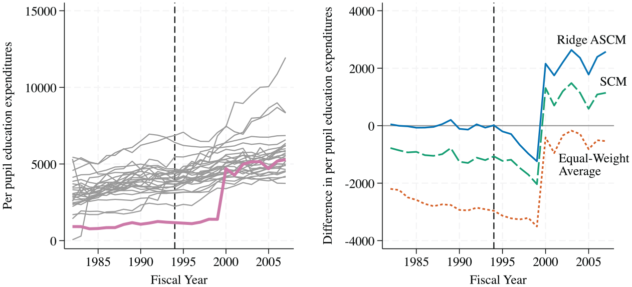
Estimating state-specific effects using Ridge ASCM and other estimation strategies.
The right panel of Figure 1 displays dynamic effect estimates of New Hampshire’s 1994 SFR on per capita education expenditures using three different comparison groups. The short-dashed orange line represents differences between New Hampshire’s per capita education expenditures and average education expenditures of nontreated states, where each nontreated state is weighted equally (referred to as “equal-weight average”). The long-dashed green line represents differences between New Hampshire’s per capita education expenditures and a synthetic control mean of education expenditures, where the synthetic control mean is calculated by assigning time-invariant weights of differing values to nontreated states based on their pretreatment match (referred to as “traditional SCM”). The solid blue line represents differences between New Hampshire’s per pupil education expenditures and a de-biased synthetic control mean of education expenditures, where the de-biased synthetic control mean is calculated by adding a bias correction term to the traditional synthetic control mean (referred to as “ridge ASCM”). In Appendix B, we include a subsection called “Bias Correction Term in the Ridge ASCM” to provide further details about the de-biased synthetic control approach.
If the comparison group adequately mirrors the pre-SFR spending levels and trend of New Hampshire, then the difference in per pupil education expenditures between the comparison group and New Hampshire should be approximately zero. As shown in Figure 1, only the ridge ASCM comparison group (blue line) consistently results in a difference, on average, of approximately zero in the pretreatment period, suggesting that the equal-weight average and traditional SCM comparison groups do not serve as good counterfactuals to New Hampshire. The use of the ridge ASCM method, therefore, serves as our preferred approach for estimating the effect of SFRs on per capita education expenditures.
RQ2: How Did Each State’s Legislature Fund Additional Education Revenues?
To identify the legislative statutes that increased state education expenditures, we used a systematic process. We began by reviewing relevant school finance history in each state using the first five sources listed in Table 1. These sources included four websites (edlawcenter.org, n.d.; schoolfunding.info, n.d.; U.S. Department of Education, National Center for Education Statistics, 2001; Verstegen, 2018) and a book documenting school finance history (Thompson et al., 2019). Collectively, these sources provided a comprehensive overview of litigation and legislative actions related to school finance in our sample of case study states. Each of these sources either provided the name of the statute that enacted the SFR or the year in which legislation altered school funding.
Reference Sources for Finding Legislative Statutes
Based on the legislative details we obtained, we conducted our search using two more steps, both of which were facilitated using the sixth source in Table 1 (congress.gov, n.d.). First, if the name of a statute was not provided, we visited the state legislature’s website. We then searched through histories of bills and acts to find the relevant statute, guided by the details we obtained from the five sources in Table 1. Second, we prioritized finding the original text of each statute. We were able to successfully find all but one original document: Kansas’ School District and Quality Performance Act (1992). In lieu of the actual text, we obtained a thorough summary of the act compiled by the Kansas Legislative Research Department. We include in-text citations of statutes we examined when discussing our results and provide the full reference with weblinks in our works cited list.
After identifying the legislative activity that was associated with each SFR, we obtained and reviewed the text of these legislative statutes and amendments for evidence of the changes legislatures made to state finances to fund increases in education spending. As needed, we also reviewed any secondary sources (i.e., academic journal articles, news articles, published briefs, or reports) we found with relevant information on how states funded SFRs. We cite all these additional sources when reporting results. Each author of this article conducted their document analysis separately and maintained analytic memos to ensure any discrepancies were addressed.
Finally, using the ridge augmented synthetic control method, we quantitatively examine the effect of a given state’s SFR on the state revenues or expenditures that were specified in legislation as being adjusted to fund increased education spending. We use the same approach to estimate the ridge ASCM as we did with RQ1, leveraging the same comparison group of states that did not have a documented SFR during our period of analysis. This second step provides an important check on whether the state legislature “followed through” and adjusted state (and, in some cases, local) finances in the ways specified in the referenced legislation.
As a robustness check for RQ2, we estimate the ridge ASCM models using a comparison group of states that had an SFR but were unable to increase and sustain expenditures after their reform. We perform this check because states with SFRs might differ in unobservable ways from those that never had a reform. As we show in Appendix E in the online version of the journal, the revenue and expenditure results are qualitatively similar to our main results, which appear in the Results section. The congruence of these results is not surprising; as noted by Shores et al. (2023), states without documented SFRs increased revenues in ways similar to states with reforms. Thus, we have suggestive evidence that our results are not driven by unobservable factors such as the propensity or motivation to engage in a finance reform.
Results
RQ1: Which States Increased and Sustained Higher Levels of Elementary-Secondary Education Spending (i.e., State Aid to School Districts) After an SFR?
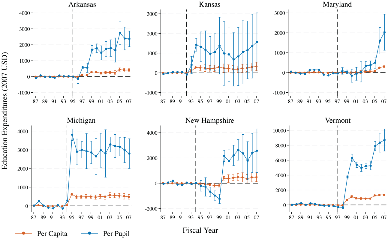
We find that 6 out of 24 state SFRs significantly increased per capita state education expenditures at the p < .05 level in the years following their first reform; therefore, they are included in our selected analytic sample. We display the ridge ASCM effect estimates of SFRs on per pupil, as well as per capita, elementary-secondary education expenditures for these six state SFRs graphically in Figure 2. For presentation purposes, we plot point estimates using 90% confidence intervals in Figure 2, given that annual dynamic effects are less precise than the average of these effects. The six state SFRs include Vermont’s Brigham v. State (FY 1997); Michigan’s Proposal A (FY 1994); New Hampshire’s Claremont School District v. Governor (Claremont I) (FY 1994); Kansas’ School District Finance and Quality Performance Act (FY 1992); Arkansas’Lake View v. Huckabee and the Equitable School Finance System Act (Act 917) (FY 1995); Maryland’s Bradford v. Maryland State Board of Education (FY 1997); and New Jersey’s Abbott v. Burke II & the Quality Education Act (FY 1991).
Ridge ASCM effect estimates of SFRs on per capita and per pupil elementary-secondary education expenditures.
As Table 2 shows, there is variation in the timing of SFRs and in their effects on state education spending. The FYs of the six SFR reforms ranged from 1992 (Kansas) to 1997 (Maryland and Vermont). The average effect of a state SFR on state education spending ranges from a high of $5,553 per pupil ($914 per capita) in Vermont to a low of $479 per pupil ($77 per capita) in Maryland.
Selected Analytic Sample of State SFRs
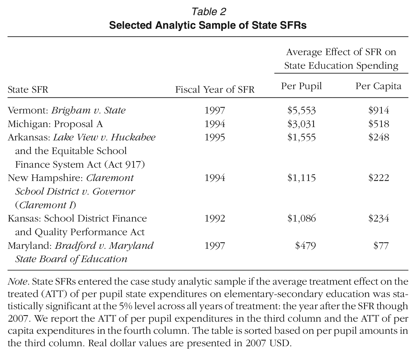
Note. State SFRs entered the case study analytic sample if the average treatment effect on the treated (ATT) of per pupil state expenditures on elementary-secondary education was statistically significant at the 5% level across all years of treatment: the year after the SFR though 2007. We report the ATT of per pupil expenditures in the third column and the ATT of per capita expenditures in the fourth column. The table is sorted based on per pupil amounts in the third column. Real dollar values are presented in 2007 USD.
Appendix Figure C1 displays ridge ASCM effect estimates of SFRs on per capita and per pupil elementary-secondary education expenditures for all 24 states that experienced an SFR between FY 1989 and 2005. For reference, Appendix Figure C2 shows the percent improvement in pretreatment model fit obtained from the per capita and per pupil elementary-secondary expenditures ridge ASCM models relative to models that use equal or traditional SCM weights.
RQ 2: How Did State Legislatures Pay for Increased and Sustained Education Spending After an SFR?
For each of the six state SFRs included in our analytic sample, we provide a brief description of the SFR and the extent to which state education expenditures increased following the SFR. We then detail how each state funded these increases in state expenditures. We begin with Vermont’s 1997 SFR, which had the largest average effect on state education funding of the six state SFRs, and we continue in descending order—Vermont, Michigan, Arkansas, New Hampshire, Kansas, and Maryland—based on the SFR’s average effect on education funding. When reporting averages of point estimates, we compute the averages using precision weighting, where the weight is the inverse of the square of the standard error.
Vermont: Brigham v. State (FY 1997)
In February 1997, the Vermont Supreme Court ruled in Brigham v. State (1997) that the state’s funding system was unconstitutional and directed the legislature to create a system that would enable “substantially equal opportunity.” In June of that same year, lawmakers enacted the Equal Educational Opportunity Act, also known as Act 60 (VT Bill H.527, 1997). Under Act 60, which went into effect in FY 1999, the legislature enabled greater equality of education funding by distributing education funds using a foundation grant program, which guarantees a base level of funding per pupil. The state also presumed the primary responsibility for funding the foundation grant program; as a result, state contributions to elementary-secondary education increased.
Districts could also opt to provide additional funding above the foundation grant by levying a local-share property tax. Funds raised from the local-share property tax were distributed using a power equalization formula, which guaranteed that districts approving the same tax rate would receive the same amount of funding per pupil, regardless of local district property wealth, through redistribution. As shown in Figure 3a, per capita state education expenditures were approximately $962 higher on average in the 9 years following Act 60’s enactment (FYs 1999–2007) compared to the state’s synthetic counterfactual.
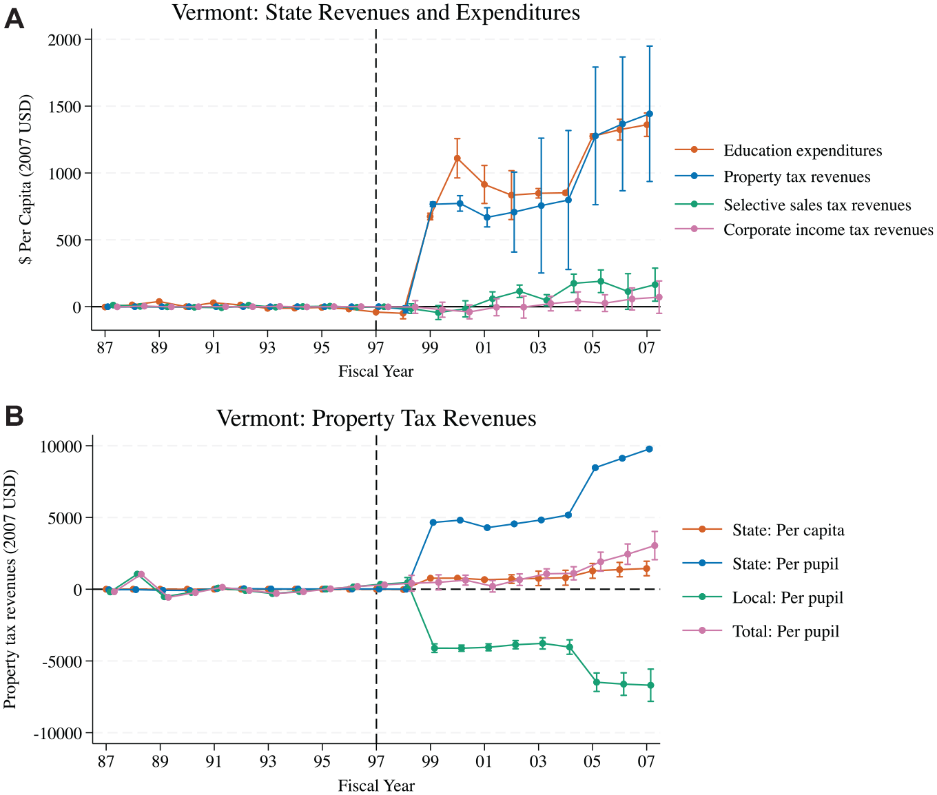
Ridge ASCM effect estimates of Vermont’s 1997 SFR: (a) ridge ASCM effect estimates of Vermont’s 1997 SFR on state revenues and expenditures; (b) ridge ASCM effect estimates of Vermont’s 1997 SFR on property tax revenues.
The Vermont legislature increased state education funding under Act 60 primarily by exerting increased control over property taxes. Specifically, the state replaced district-controlled local property taxes with a state-controlled state property tax. As a result, per capita state property tax revenues increased by approximately $763 on average—per pupil property tax revenues increased by $5,348 on average—relative to Vermont’s synthetic control group in the years following Act 60’s passage (FYs 1999–2007; see Figure 3b). In contrast, local property tax revenues decreased over the same period; per pupil property tax revenues decreased by $4,180 on average. Total property tax revenues—the sum of state and local property tax revenues—remained largely unchanged following Act 60’s enactment.
Act 60 also raised additional state education funding by mandating small increases to a variety of taxes, including the rooms and meals sales tax (2 percentage point increase), motor fuels sales tax (4 cent increase), purchase and use tax on motor vehicles (1 percentage point increase), sales tax on telecommunication services (imposing a 4.36% tax), corporate income tax (1.5 percentage point increase), and bank franchise tax and brokerage fees. Corporate income tax revenues and selective sales tax revenues (which encompass many of the tax increases mentioned above) increased post-1997, though these effects are not consistently significant (see Figure 3a).
Finally, Act 60 also specified that lottery revenues be used solely for funding elementary-secondary public education. Consequently, lottery revenues were to be placed in the education fund, rather than the general fund. Because Vermont’s lottery revenues were only about $50 per capita on average between 1999 and 2007, diverting lottery funds from the general fund to the education fund likely had negligible effects on funding for other state priorities, including welfare, corrections, and higher education. We also do not find quantitative evidence that noneducation state expenditures decreased post-1997 in Vermont.
Michigan: Proposal A (FY 1994)
In 1993, the Michigan State Legislature and governor eliminated local property taxes as a source of funding for education, which state politicians and citizens had been attempting to do since the early 1970s (Courant & Loeb, 1997). To fund education, the legislature proposed—and voters subsequently approved—a constitutional amendment, Proposal A, in FY 1994 (MI Senate Joint Resolution S, 1993). As depicted in Figure 4a, per capita education spending was $532 higher, on average, in Michigan post-1994 compared to its synthetic counterfactual.
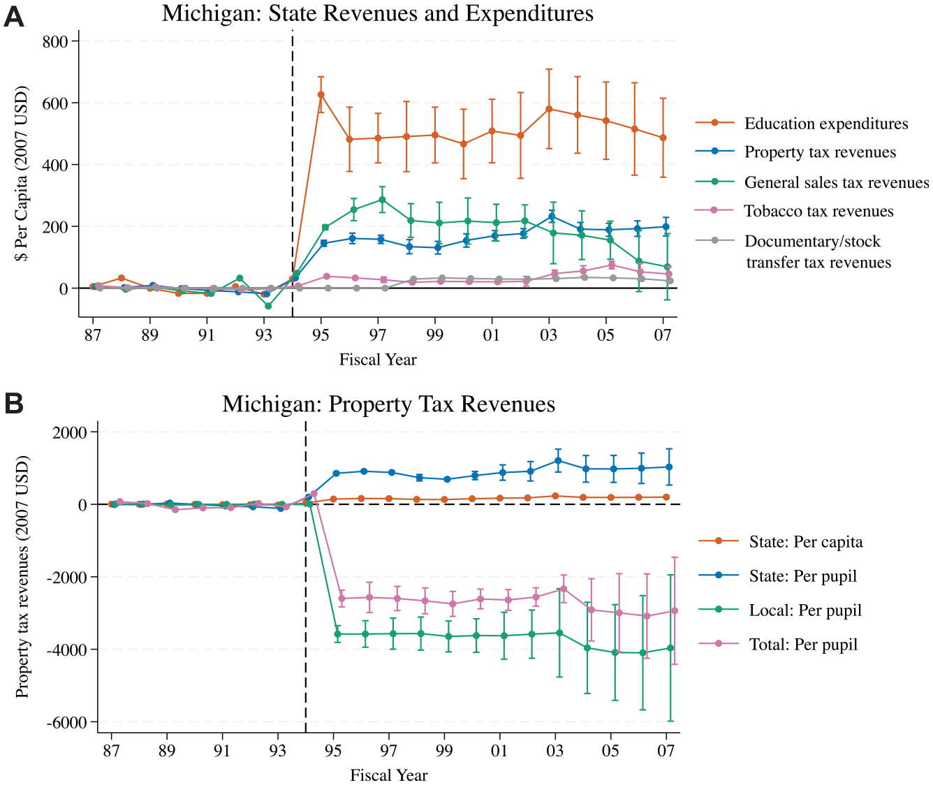
Ridge ASCM effect estimate of Michigan’s 1994 SFR: (a) ridge ASCM effect estimates of Michigan’s 1994 SFR on state revenues and expenditures; (b) ridge ASCM effect estimates of Michigan’s 1994 SFR on property tax revenues.
Proposal A led to increased state education expenditures by altering Article 9 (Finance and Taxation) of the Michigan state constitution and changing the tax systems that raised revenues for schools. Specifically, Proposal A required that the sales and use tax be raised by 2 percentage points and that a new state property tax of 6 mills be enacted. As a result, Michigan’s state general sales tax revenues were about $201 higher per capita in Michigan post-1994, while state property tax revenues were approximately $165 higher per capita ($843 higher per pupil; see Figure 4b). Proposal A also set limits on the minimum and maximum property tax rates that could be imposed locally. Consequently, local property tax rates and revenues declined on average by $3,605 per pupil, as well as total—the sum of state and local—property tax rates and revenues by $2,610 per pupil; see Figure 4b. Thus, Proposal A ultimately resulted in property tax relief for Michigan citizens.
Proposal A also increased the cigarette tax by 50 cents per pack, and the real estate transfer tax increased by 0.45 percentage points. As shown in Figure 4a, these tax changes led to small increases in the state tobacco tax—$27 per capita, on average—and in documentary and stock tax revenues—$4 per capita, on average. We note that our measure of documentary and stock tax revenues includes real estate transfer tax revenues, as the Census Bureau does not provide a separate measure of them.
All revenues generated from the Proposal A tax increases were earmarked for the state School Aid Fund and then distributed by the state to school districts based on a foundation grant formula (Courant & Loeb, 1997). Districts that raised more than the base foundation grant with the required local property tax rate were not required to return the excess revenue to the state, though the state did cap revenues in previously high-spending districts based on 1994 revenue levels (Cullen & Loeb, 2004). Certain high-wealth districts were also able to raise additional funding above the foundation grant via hold harmless mills.
Arkansas: Lake View v. Huckabeeand the Equitable School Finance System Act (FY 1995)
In December 1994, the court declared in Lake View v. Huckabee (1994) that Arkansas’ state education funding system was unconstitutional and that the state had 2 years to enact a new funding scheme. In February 1995, the Arkansas General Assembly approved the Equitable School Finance System Act, more commonly known as Act 917 (AR Act 917, 1995). Under Act 917, which went into effect in FY 1997, the General Assembly implemented an equalization school funding formula. Equalization plans typically supplement local funding by providing a block grant to districts based on certain characteristics, such as local tax base or revenues (Shores et al., 2023). In the 11 years following Act 917’s passage (FYs 1997–2007), Arkansas’ per capita state education funding increased by $208, on average, relative to its synthetic counterfactual (see Figure 5a).
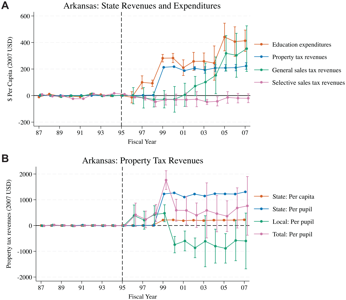
Ridge ASCM effect estimates of Arkansas 1995 SFR: (a) ridge ASCM effect estimates of Arkansas 1995 SFR on state revenues and expenditures; (b) ridge ASCM effect estimates of Arkansas’ 1995 SFR on property tax revenues.
Act 917 enabled increased state education funding by replacing local property tax rates that varied by district with a state-controlled uniform property tax rate or “base millage rate.” The state both collected and redistributed the revenues which were raised from the uniform property tax. As shown in Figure 5b, per capita state property tax revenues increased by approximately $117 on average (per pupil property tax revenues increased by $555 on average) relative to Arkansas’ synthetic control group after Act 917’s enactment (FYs 1997–2007). In contrast, local property tax revenues decreased over the same time period (per pupil property tax revenues decreased by $245 on average). Total (local plus state) property tax revenues increased by $655 per pupil on average following HB Act 917’s passage (FYs 1997–2007).
Based on our legislative document search, we also found that the General Assembly further increased state education funding in February 2004 by passing Act 107 during the Second Extraordinary Session of 2003 (AR Act 107, 2004). Effective in March of 2004, Act 107 increased the state sales and use tax rate by 0.875%, expanded the services that the state general sales tax applies to, and increased the wholesale vending tax to provide additional revenues for elementary-secondary education. Descriptively, we find that per capita general sales tax revenues increased by $324, on average, between 2005 and 2007 compared to Arkansas’ synthetic counterfactual (see Figure 5a). However, we do not find that selective sales tax revenues (which includes wholesale vending tax revenues) significantly increased in Arkansas after Act 107’s enactment (FYs 2004–2007) relative to the state’s synthetic control. This is likely due to wholesale vending tax revenues making up a small proportion of selective sales tax revenues. As shown in Figure 5a, between 2005 and 2007, Arkansas’ per capita state education funding had risen by $419 relative to the synthetic control group.
New Hampshire: Claremont School District v. Governor (Claremont I) (FY 1994)
In FY 1994, the New Hampshire Trial Court ruled in Claremont I (1994) that the state has a constitutional duty to provide each child with an adequate education. Three years later, in December of 1997, the New Hampshire Supreme Court further declared in Claremont II (Claremont v. Governor, 1997) that the state education finance system was unconstitutional because it enabled inequitable local property tax rates and fostered inadequate educational opportunities. The court ordered that the state needed to define and fund what constituted an adequate education. In response to the Claremont rulings, the state legislature eventually passed House Bill (HB) 117 in April 1999 after several failed reform plans (NH H.B. 117, 1999). HB 117 established a foundation grant program for distributing education funding. In the eight years following HB 117’s passage (FYs 2000–2007), New Hampshire’s per capita state education funding increased by $420, on average, relative to its synthetic counterfactual (see Figure 6a).
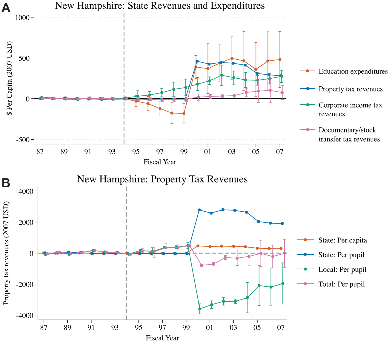
Ridge ASCM effect estimates of New Hampshire’s 1994 SFR: (a) ridge ASCM effect estimates of New Hampshire’s 1994 SFR on state revenues & expenditures, (b) ridge ASCM effect estimates of New Hampshire’s 1994 SFR on property tax revenues.
HB 117 enabled increased state education funding by replacing district-controlled local property taxes with a state-controlled state property tax. School districts were required to give excess property revenue to the state government if their state property tax revenue was greater than the base foundation grant; however, districts were also allowed to spend more than the base foundation grant by levying additional local property taxes (Lutz, 2010). As shown in Figure 6b, per capita state property tax revenues increased by approximately $424 on average (per pupil property tax revenues increased by $2,438 on average) relative to New Hampshire’s synthetic control group after HB 117’s enactment (FYs 2000–2007). In contrast, local property tax revenues decreased over the same time; per pupil property tax revenues decreased by $3,180, on average. Together, the sum of local and state property taxes decreased following HB 117’s enactment.
HB 117 also increased funding for education by mandating smaller increases to a variety of state taxes, including raising the business enterprise and business profits tax, raising the real estate transfer tax, expanding the rooms and meals sales tax, and instituting a statewide property tax on utility properties. In turn, corporate income tax revenues (which includes business enterprise and business profits tax revenues) and documentary and stock transfer tax revenues (which includes real estate transfer tax revenues) increased in New Hampshire after HB 117’s enactment relative to the state’s synthetic control (see Figure 6a). We do not find that selective sales tax revenues (which include rooms and meals sales tax revenues) significantly increased in New Hampshire after HB 117’s enactment (FYs 2000–2007) relative to the state’s synthetic control. This is likely due to the rooms and meals sales tax revenues making up a small proportion of selective sales tax revenues. The bill also dedicated revenues from future increases in the tobacco tax to the education trust fund and designated certain tobacco settlement funds received by the state for education funding.
Kansas: The School District Finance and Quality Performance Act (FY 1992)
Throughout the late 1980s and early 1990s, 42 Kansas districts filed four separate legal challenges regarding the constitutionality of the current state school finance system under the School District Equalization Act (SDEA). These legal challenges were consolidated into one case, and in 1991, a district court judge indicated in a pretrial ruling that if the case went to trial, he would likely declare that the SDEA violated the state constitution’s requirement that the legislature “make suitable provision for finance of the educational interests of the state” (Mock v. State, 1991). Subsequently, the Kansas Governor, Joan Finney, established a task force for determining a new state school funding formula.
In 1992, the Kansas Legislature passed the School District Finance and Quality Performance Act (SDFQPA) (KS H.B. 2892, 1992). The SDFQPA, which went into effect in FY 1994, established a foundation grant program. In addition, a provision of SDFQPA, known as the Local Option Budget (LOB), permitted districts to raise additional funding 25% above the base foundation grant if approved by local citizens (Johnston & Duncombe, 1998; Thompson & Clark, 2001). The funding scheme also included a variety of special weightings or cost adjustments to accommodate differences in district characteristics and differences in the student populations served by districts. In the 14 years following the SDFQPA’s enactment (FYs 1994–2007), Kansas’ per capita state education expenditures were approximately $249 higher on average compared to the state’s synthetic counterfactual (see Figure 7a).
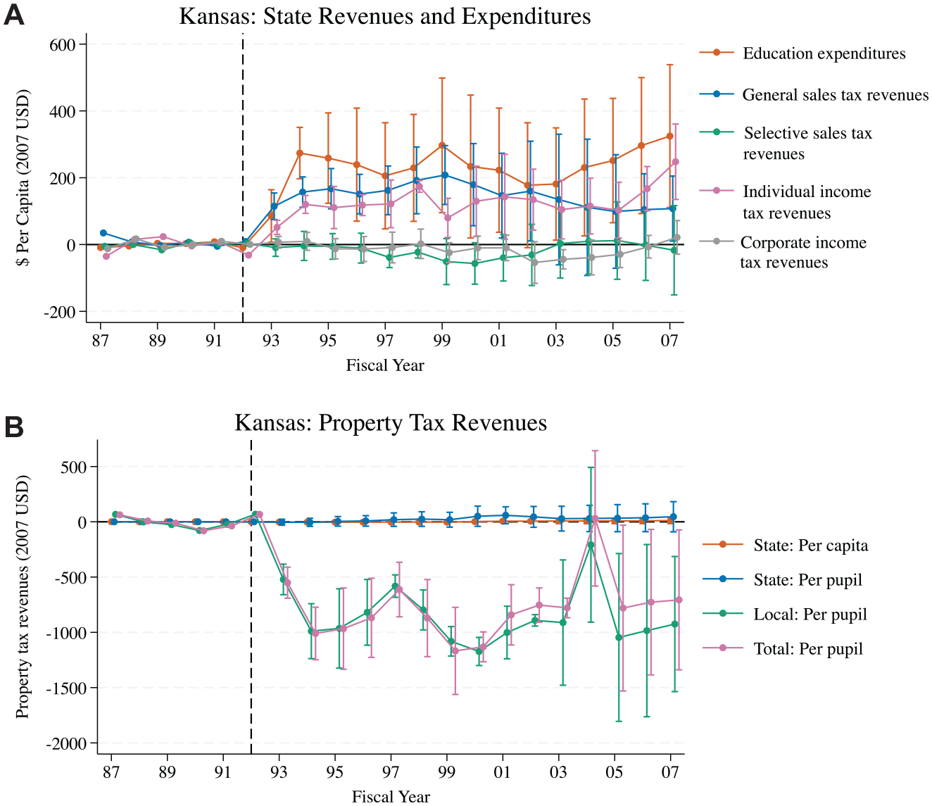
Ridge ASCM effect estimates of Kansas’ 1992 SFR: (a) ridge ASCM effect estimates of Kansas’ 1992 SFR on state revenues and expenditures; (b) ridge ASCM effect estimates of Kansas’ 1992 SFR on property tax revenues.
The SDFQPA increased state education expenditures by raising state tax revenues while simultaneously reducing local property tax burdens. State tax increases included raising the state general sales tax rate (from 4.25% to 4.9%), enacting higher individual and corporate income tax rates, and eliminating various sales tax exemptions (Johnston & Duncombe, 1998; Thompson & Clark, 2001). As shown in Figure 7a, increased general sales and individual income tax revenues enabled the bulk of new education funding, with general sales tax revenues increasing by $157 on average and individual income tax revenues increased by $144 on average in the years post-SDFQPA (FYs 1994–2007). As also shown in Figure 7a, selective sales tax and corporate income tax revenues were not statistically different from those of Kansas’ synthetic counterfactual.
The SDFQPA also required districts to impose a uniform local property tax rate, which was 32 mills in 1992; 33 mills in 1993; 35 mills in 1994 through 1996; 27 mills in 1997; and 20 mills in 1998 (Thompson & Clark, 2001). The imposition of the uniform local property tax rate resulted in lower local property tax revenues—a decrease of $888 per pupil on average (see Figure 7b)—and property tax relief for citizens. If local property tax revenues were greater than a district’s base foundation grant, the excess local revenues were remitted to the state and then redistributed to other “property poor” districts (Johnston & Duncombe, 1998; Thompson & Clark, 2001).
Maryland: Bradford v. Maryland State Board of Education(FY 1997)
In FY 1997, the court ruled in Bradford v. Maryland State Board of Education (1996) that students in Baltimore City public schools were not receiving a constitutionally adequate education; thereafter, Maryland’s General Assembly and governor established a commission to study the school finance system of Maryland and calculate the cost of providing an adequate education. The commission’s formal name was the Commission on Education Finance, Equity, and Excellence, but it was also referred to as the Thornton Commission after its chairman, Alvin Thornton. In January 2002, the commission issued its final recommendations, which included revising the state school funding formula and increasing state education expenditures by $1.1 billion (Commission on Education Finance, Equity, and Excellence, 2002).
Based on the commission’s recommendations, the Maryland General Assembly passed the Bridge to Excellence in Public Schools Act (SB 856) in FY 2002 (MD S.B. 856, 2002). The Bridge to Excellence (BTE) Act implemented a foundation program funding scheme, where districts were provided with a uniform per pupil base amount of funding that the state estimated to be the minimum amount required to provide an adequate education. BTE also called for an increase in state education funding, especially in districts with large populations of children from educationally disadvantaged backgrounds, which was to be phased in over 6 years. As shown in Figure 8a, per capita education spending subsequently increased in Maryland in the 5 years following the passage of BTE. We do not examine state education expenditures in the 6th year (FY 2008) because our fiscal data set ends FY 2007, the last FY prior to the Great Recession. Per capita state education expenditures were approximately $132 higher on average in FYs 2003 to 2007 compared to Maryland’s synthetic counterfactual.
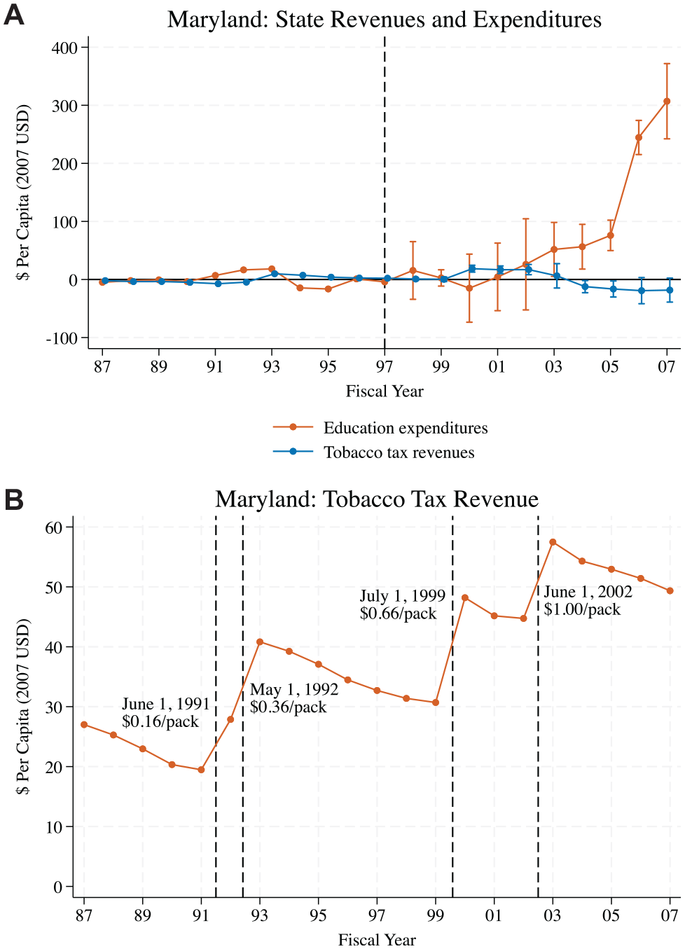
Ridge ASCM effect estimates of Maryland’s 1997 SFR and time series of tobacco tax revenues: (a) ridge ASCM effect estimates of Maryland’s 1997 SFR on state revenues and expenditures; (b) time series of tobacco tax revenues.
BTE required taxes on cigarettes to be raised from 66 cents to $1 per pack in FY 2003 to fund the 1st year of increased state education expenditures. Tobacco tax revenues and education expenditures subsequently increased in FY 2003; see Figure 8a. While tobacco tax revenues did not significantly increase in FY 2003, the confidence intervals associated with the FY 2003 tobacco tax effect estimate and elementary-secondary education effect estimate overlap. Thus, we cannot reject the possibility that tobacco tax revenues and education expenditures in Maryland rose by similar amounts in FY 2003. However, the Act did not specify a revenue source to fund the remaining 5 years (FYs 2004–2008) of mandated education spending increases. In Maryland, an act does not have to identify a revenue source for future proposed spending, per a 1978 amendment to the state constitution (Norcross, 2011).
Additional searches based on state finance documents and news articles on BTE and Maryland state education funding during this time did not yield any additional details regarding revenue sources. However, as we show descriptive in Figure 8b, the elevated tax revenues from the cigarette tax increase likely continued to fund education. We also examined the effects of Maryland’s SFR on other state revenue and expenditure categories using ridge ASCM but did not find any evidence of funding sources that could be corroborated with legislative documents.
Discussion
We find that five of the six state SFRs examined in this study—Vermont (1997), Michigan (1994), Arkansas (1995), New Hampshire (1994), and Kansas (1992)—were funded by altering tax rates and changing tax revenue sources. These five states paid for increased education expenditures by increasing a variety of state tax revenues, such as general and selective sales taxes and individual and corporate income taxes. While none of these five state legislatures altered the exact same set of tax revenues, suggesting there is no single “recipe” for funding SFRs, they did share a common approach with respect to property taxes: All five states increased state education spending by increasing state control over the imposition, collection, or distribution of property tax revenues. Consequently, local property tax revenues decreased in all five states. State property tax revenues, however, only increased in four states: Vermont, Michigan, Arkansas, and New Hampshire.
Maryland funded increased state education spending for 1 year by raising tobacco tax revenues, but we were unable to determine how the state funded the remaining 5 years of mandated education spending increases using the ridge ASCM approach. Legislative documents were not helpful because Maryland’s state constitution does not require the legislature to identify a revenue source for proposed spending in the future (Norcross, 2011). Our descriptive time series of Maryland’s tobacco tax revenues (Figure 8b), however, does suggest that the increased revenue from the cigarette tax sustained funding through the end of our sample period. Thus, in the case of Maryland, multiple approaches—the combination of legislative document analysis, ridge ASCM, and descriptive time series graphs—were needed to understand how the legislature likely funded increases in state education spending.
The five states that increased control over property tax revenues and raised a variety of other state tax revenues experienced larger average increases in state education funding compared to Maryland, which only increased one, non-property-tax revenue. Specifically, as shown in Table 2, the average estimated effect of a state SFR reform on state education spending was $77 per capita in Maryland. In contrast, the average estimated effect of an SFR on state education funding ranged from $222 to $914 per capita in Arkansas, Kansas, Michigan, New Hampshire, and Vermont. These findings suggest that larger increases in state education funding are achieved when legislatures (a) increase multiple tax revenue streams, including sales and excise taxes; and (b) exercise more control over property taxes. Our results align with prior research, indicating that reforms are funded by tax revenues (Liscow, 2018); however, our study documents the specific sources of these tax revenues and identifies their contribution to funding.
Policy Considerations
Distribute State Aid Equitably
Although a primary objective of many SFRs is to increase state education expenditures for elementary-secondary education, policymakers should also consider how to equitably distribute these funds to school districts (Downes & Pogue, 1994; Duncombe & Yinger, 1998). Districts receive state expenditures for education as state aid in their revenue accounts via an intergovernmental transfer, so the allocation of these funds matters for their district-level budgeting and planning (Odden & Picus, 2020). If policymakers were to allocate a disproportionate amount of state aid to wealthy districts, they might exacerbate the inequality of education funding driven by local property wealth (Chetty & Friedman, 2010), undermining any desired equity goals of an SFR. Alternatively, allocating additional state aid to districts with lower property wealth or more economic disadvantage could work to increase funding in these districts, which research shows translates to improved student outcomes (Candelaria & Shores, 2019; Jackson et al., 2016; Lafortune et al., 2018).
Several approaches exist for distributing state aid, ranging from distributing funds according to enrollment to targeting aid based on need (Morgan & Pelissero, 1989; Odden & Picus, 2020). One concrete example of a distribution mechanism, which was recently adopted in Tennessee because of their legislative SFR in 2022, is a weighted student funding formula (WSFF). The state’s WSFF gives each student a base funding amount and provides additional funding according to selected demographic characteristics as shares of the base amount—the so-called weights (Odden & Picus, 2020; Tennessee Department of Education, 2023). However, given that state aid is ultimately constrained by the revenue sources that fund it, any distribution mechanism, including WSFF, will involve tradeoffs about which student demographic groups should receive additional funding (e.g., economically disadvantaged students, English language learners, students with unique learning needs) and what proportion of funding goes to each group (Candelaria et al., 2023).
Account for the Preferences of Local Taxpayers
The preferences of local taxpayers matter because these taxpayers fund the local share of revenue that school districts receive (Barlow, 1970; Loeb, 2001). For school districts, the two largest revenue sources for their budget are state aid and local funding, as federal aid typically comprises a small share (Howell & Miller, 1997). The response of local taxpayers to an SFR warrants consideration from policymakers, as it affects the total funding districts receive. As shown in Figure 9, the effects of SFRs on local funding are quite heterogenous. Even though per pupil state spending increases—a mechanical artifact based on our case study selection approach—local funding decreased significantly in Kansas, Michigan, New Hampshire, and Vermont. Indeed, this is not completely surprising as these states absorbed control of property taxes for the purpose of redistribution. However, New Hampshire’s local funding decrease is notable given that the sum of local and state revenues decreased in the years after reform. One explanation for the sharp decrease in local funding is that local taxpayers engaged in a tax revolt in response to their SFR (Dandurant, 2000).
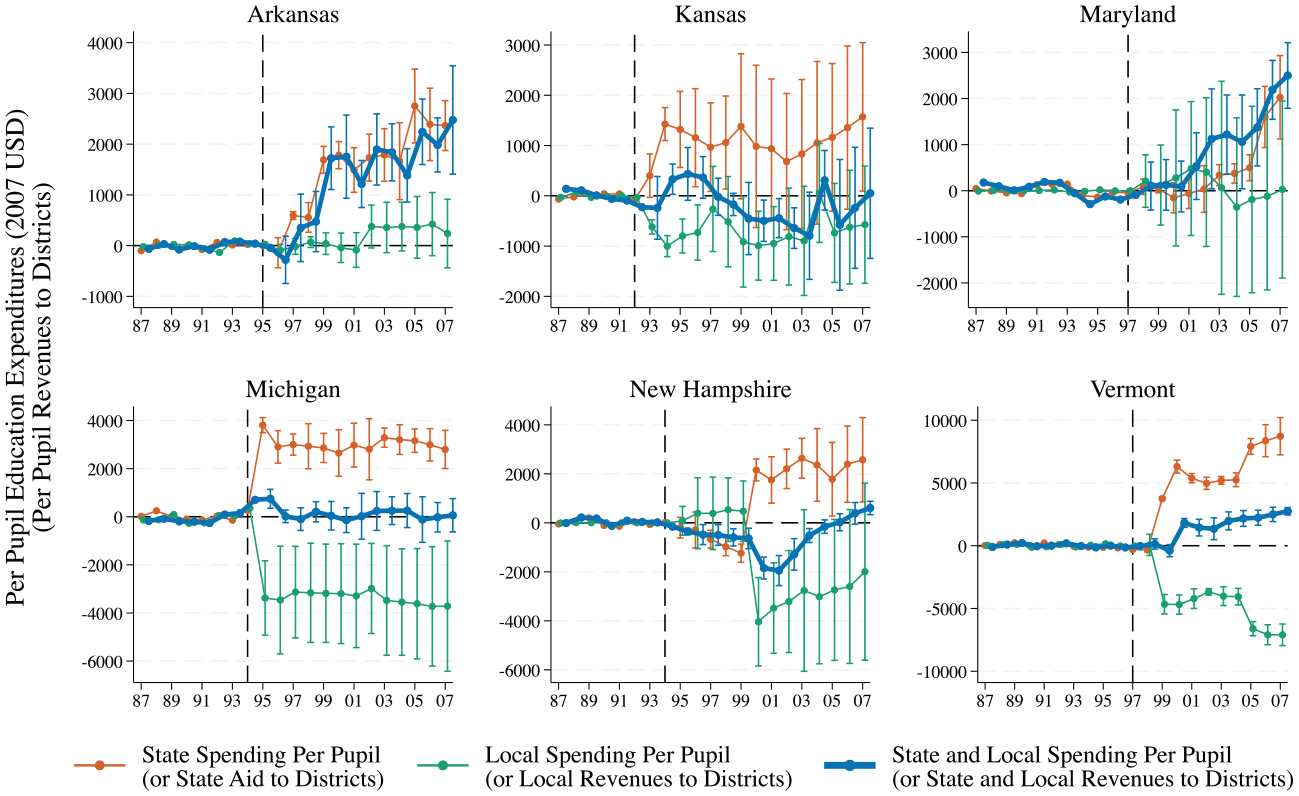
Ridge ASCM effect estimates of SFRs on state and local expenditures per pupil.
When local taxpayers face significant tax increases, there might be potential resistance to support education through fiscal effort (Hoxby, 2001; Rockoff, 2010; Steinberg et al., 2016). Therefore, assessing the impact of SFRs requires a comprehensive view of total revenues, particularly if the aim is ensuring adequate funding for students, which requires examining total revenue. State aid alone may not suffice if local funding substantially drops. SFR funding policies will need to account for the preferences of local voters to gauge whether they are likely to support education reform through additional fiscal effort, seek property tax relief, or engage in a tax revolt.
Assess Budgetary Tradeoffs
Finally, we think it is important for policymakers to assess budgetary tradeoffs—reducing noneducation expenditures or increased state debt—associated with funding SFRs (Baicker & Gordon, 2006; Liscow, 2018). We find no legislative evidence, based on our document analysis, that noneducation state expenditures were reduced or that state debt was increased to fund increased elementary-secondary education spending following an SFR. However, one may wonder if we find no evidence of reduced noneducation expenditures or increased debt because such things are not mentioned in legislative statutes related to increasing education funding—either because they are not required to be mentioned or because doing so might have negative ramifications.
To assess whether noneducation expenditures decreased or whether state debt increased, we estimated the effects of the six state SFRs on per capita noneducation state expenditures and total state debt outstanding using ridge ASCM. As described in detail in Appendix D in the online version of the journal, while we do find some evidence that noneducation state expenditures were reduced and state debt increased in the years following an SFR in a few states, we were unable to verify or corroborate such findings using other sources of information (e.g., academic journal articles, news articles, published briefs, or reports). Without additional corroborating evidence, we are not confident that the effects on noneducation expenditures and state debt should be attributed to SFRs (versus other events or policy changes that occurred at the same time). As such, we recommend further examination into whether SFR-induced increases in state education spending impact the funding of other state priorities or state deficits.
Overall, we acknowledge that these patterns we observe in this study are based on a small sample of six state SFRs and thus should be interpreted with caution. Future research should examine the relationship between how SFRs are funded and the magnitude of the increase in state education spending using a larger sample of state SFRs.
Conclusion
Prior research suggests that potential avenues for funding SFRs include increasing revenues by raising taxes; reducing expenditures on other state priorities such as welfare, corrections, and higher education; or increasing state debt (Baicker & Gordon, 2006; Liscow, 2018). However, because states have different political environments, funding priorities, and tax systems, the ways in which SFR-induced increases in education expenditures are funded likely vary across states. Our study is the first to examine how individual states funded these increased expenditures using synthetic control methods and document analysis.
We use a novel, multistep approach to determine how SFRs are funded, drawing on evidence from multiple sources (both legislative acts and quantitative finance data). Referencing relevant legislative statutes provided a very detailed accounting of (a) which specific state revenue categories were changed and (b) to what degree (e.g., how many percentage points a given tax rate was raised). We were also able to verify the impact of this legislative change by quantitatively examining the effect of a state’s SFR on the given revenue categories using state finance data and ridge ASCM (Ben-Michael et al., 2021). Research designs focusing exclusively on quantitative analyses of state finance data lack the detailed insights that can be gained from legislative review.
Although our analysis focuses on the adequacy era before the Great Recession, SFRs continue to be relevant in education policy discussions. There have been at least 10 court-ordered finance reforms that have resulted in a state high court requiring the legislature to either change their finance system or add additional funding (Hanushek & Joyce-Wirtz, 2023). In one prominent case, McCleary, et al. v. State of Washington, the state supreme court declared Washington’s education funding system unconstitutional in 2012. Although the ruling occurred in 2012, the state did not satisfy the court order until the 2018–2019 school year when lawmakers enacted a bill substantially increasing state aid (Sun et al., 2024). Independent of a court order, states may also choose to pursue finance reforms to overhaul their education funding systems. For example, Tennessee policymakers recently enacted the Tennessee Investment in Student Achievement Act into law in 2022, introducing a weighted student funding formula for distributing state aid to districts. These examples reveal that SFRs are not policy relics of the past; rather, they underscore the need for further research that examines the granular details of these reforms, including how they are funded.
The search for funding is likely a barrier that policymakers face and is one possible explanation for why some SFRs did not result in increased education funding (Shores et al., 2023). Understanding the breadth of options available for increasing education expenditures will inform state and education policymakers about different approaches for supporting education spending in their own states. From a budgetary perspective, our analyses find that our case study states did not increase state debt or require reducing noneducation expenditures. However, as we caution in our discussion, funding an SFR is only one part of the process. Policymakers must also consider the extent to which state aid is equitably distributed across districts as well as the extent to which local funding may change based on the preferences of taxpayers residing in the state, especially if the goal is to increase the sum of local and state aid to reach a funding target threshold.
Supplemental Material
sj-pdf-1-aer-10.3102_00028312241264320 – Supplemental material for Paying for School Finance Reforms: How States Raise Revenues to Fund Increases in Elementary-Secondary Education Expenditures
Supplemental material, sj-pdf-1-aer-10.3102_00028312241264320 for Paying for School Finance Reforms: How States Raise Revenues to Fund Increases in Elementary-Secondary Education Expenditures by Shelby M. McNeill and Christopher A. Candelaria in American Educational Research Journal
Footnotes
Notes
S
C
References
Supplementary Material
Please find the following supplemental material available below.
For Open Access articles published under a Creative Commons License, all supplemental material carries the same license as the article it is associated with.
For non-Open Access articles published, all supplemental material carries a non-exclusive license, and permission requests for re-use of supplemental material or any part of supplemental material shall be sent directly to the copyright owner as specified in the copyright notice associated with the article.