
Abstract
Observation Oriented Modeling is an alternative to traditional methods of data conceptualization and analysis that challenges researchers to develop integrated, explanatory models of patterns of observations. The focus of research is thus shifted away from aggregate statistics, such as means, variances, and correlations, and is instead directed toward assessing the accuracy of judgments based on the observations in hand. In this paper a number of example data sets will be used to demonstrate how Observation Oriented Modeling can be taught to undergraduate and graduate students. While the examples are drawn from psychology, the method of contrasting Observation Oriented Modeling with traditional methods of research design and statistical analysis can easily be adapted to examples from other sciences.
Overview
Observation Oriented Modeling (Grice, 2011) is a novel and intuitive approach for both conceptualizing and analyzing data in the social and biological sciences. Imagine a scientist, for instance, studying a mother and child interacting in a laboratory. Countless observations can be made regarding the mother and child in this artificial setting. Physical characteristics such as height and weight can readily be measured, behaviors such as talking and touching can be directly observed, and qualities such as parenting style or child temperament may be inferred from other observable behaviors. The goal of the observation-oriented scientist is to construct an explanatory model for the observations being made, and this goal is equivalent to seeking the causal structure of the natural system under investigation. In other words, the observation oriented scientist assumes that the persons, physical features, behaviors, and qualities directly or indirectly observed are organized or oriented toward one another in consistent and knowable ways because of nature's causal structure.
Of course no scientist is a passive observer or tabula rasa; therefore, observations are structured and ordered the way they are in part because of the scientist's judgments. Placing toys or magazines in the room, for instance, may affect the mother-child interaction and the subsequent observations. Decisions must also be made regarding which physical features or behaviors are to be observed and how they are to be recorded, and methods must be derived for assessing qualities that are not directly observable. To insure that his or her model captures the causal structure of nature accurately, then, the observation-oriented scientist must also be oriented toward the many assumptions and decisions that go into making observations. As an example, consider the commonplace strategy among personality psychologists of summing responses from multiple-item inventories to obtain trait scores. This procedure assumes that personality traits are structured as continuous quantities and can be measured as such, even though no scientific evidence exists for this latter assumption (Michell, 2011). For the observation-oriented scientist this is an untenable position. Either evidence must be gathered to support the continuity claim or the various models of traits must be altered to provide a more accurate view of reality. The latter approach would require personality psychologists to return to the question “What is a personality trait?” and to devise novel methods of observation in conjunction with their new models.
To accomplish the goal of constructing a model that accurately captures the causal structure of nature, the observation-oriented scientist must furthermore steer away from the modern paradigm of statistical modeling. This paradigm is perhaps epitomized by structural equation and path diagrams that connect constructs and variables in networks of associations. The variables in these diagrams are often assumed to represent continuous quantities and their analysis is consequently based on aggregate statistics, such as means, variances, and covariances. Their efficacy is moreover almost universally assessed via the estimation of abstract population parameters in the assumption-laden context of null hypothesis significance testing (i.e., via p values). In contrast, the observation-oriented scientist must be willing to get beyond these methods and re-orient his or her attention to the observations being made and to the individuals being studied. Rather than compute aggregate statistics and estimate population parameters, patterns of observations are instead examined in light of a causal model using analysis techniques that are relatively free of assumptions and yield results that are both transparent and interpretable at the level of the individuals in the study. The overall analysis objective is thus to assess the accuracy of a model as an explanation of patterns of observations.
As a novel approach for conceptualizing and analyzing data, the use of Observation Oriented Modeling requires something of a Gestalt shift on behalf of the scientist trained in contemporary experimental statistics. The purpose of this paper is to facilitate this shift by providing instructional information and class projects to teach Observation Oriented Modeling to graduate and advanced undergraduate students in the life sciences. The information and projects presented below are likely most suitable for an existing course on experimental statistics or research methods, and the example analyses can be taught alongside traditional methods of data analysis. In fact, the example analyses below compare and contrast traditional methods with Observation Oriented Modeling.
As will be made plain below as well, however, a basic knowledge of the different philosophical schools of thought (e.g., positivism, realism, idealism) is required of the instructor. Accordingly, important concepts and ideas that must be taught to students are discussed generally, and they are also specifically presented before each example project. The projects themselves are based on genuine or contrived studies and are designed to demonstrate: (1) the application of key concepts; (2) the development of integrated, causal models; and (3) how data can be analyzed with the Observation Oriented Modeling (OOM) software. 2 The examples are drawn from the psychological literature but students from other life sciences (e.g., biology, sociology, education) should find them accessible and meaningful as well. We begin with an explanation of the impetus behind the development of Observation Oriented Modeling.
Why Observation Oriented Modeling?
The majority of students today are taught that psychological research can be subdivided into three areas: statistical analysis, research design, and measurement. As revealed in a recent review of doctoral programs in the United States by Aiken, West, and Millsap (2008), students receive more training in statistics than either research design or measurement, although Aiken, et al. are quick to point out that training in all three areas is inadequate. They also imply in their review that insufficient training – coupled with declining numbers of quantitative psychologists – will have a decidedly negative effect on the overall quality of future research in psychology. It could in fact be argued that the predicted decline in quality has already occurred, as recent scholarly critiques have highlighted a general lack of understanding among modern researchers with regard to fundamental issues of statistics (particularly the p value; Gigerenzer, 2004; Lambdin, 2012), research design (Lebel & Peters, 2011), and measurement (Michell, 2008, 2011). Highly publicized critiques have moreover spotlighted psychologists' general neglect of fundamental principles of scientific investigation, particularly the importance of exact replication and the value of critical discourse among colleagues (Lehrer, 2010; Alcock, 2011; Yong, 2012; Abbott, 2013).
While these recent critical appraisals may seem to support Aiken, et al.'s call for more quantitative training, other scholars have drawn attention to a deeper set of issues that must first be addressed. Joseph Rychlak (1985, 1988) argued nearly thirty years ago that psychologists have a tendency to permit their methods to drive their metaphysics (their general view of human nature), whereas in proper scientific investigation methods must be devised according to a suitable metaphysics. David Bakan (1967) referred to this error more forcefully as “methodolatry” – the irrational belief that nature should conform to research methods rather than the other way round. In the domain of statistics, David Freedman, author of one of the most highly regarded textbooks on statistics (Freedman, Pisani, & Purves, 2007), argued for a return to simpler statistical methods with greater emphasis placed on sound theorizing and sleuth-like detective work (1991; see also Mason, 1991). Psychologists' tendency to idolize complex statistical methods at the expense of sound reasoning was more recently dubbed “statisticism” by James Lamiell (2013), which fits well with other descriptions of modern statistical analysis as “sorcery” (Lambdin, 2012), “mindless” (Gigerenzer, 2004), and “inevitable and useless” (Toomela, 2010). With regard to measurement, Joel Michell has argued persuasively that psychologists have, since the early 1900s, avoided the fundamental issue of measurement; namely, the establishment of additive units of measure for the psychological attributes they study. The consequent being, “There is no evidence that the attributes that psychometricians aspire to measure (such as abilities, attitudes and personality traits) are quantitative” (Michell, 2011, p. 245). If Michell's assessment is correct, then psychologists have been using and advocating methods that often presume continuous quantities (e.g., ANOVA, SEM, IRT, etc.) where no evidence exists that the qualities or attributes they study are in fact continuous. Again, this is an instance of psychologists allowing their methods to drive their metaphysics.
The premise underlying the development of Observation Oriented Modeling and the OOM software is that the arguments of methodolatry and statisticism are essentially correct; and they are correct because psychology has built its research methods foundation primarily upon the tenets of philosophical positivism, which is a viewpoint steeped in phenomenalism and long ago abandoned by philosophers due to its many additional inadequacies (see Costa & Shimp, 2011). What is currently needed, then, is a way of thinking about research that does not necessarily entail training in contemporary statistical methods or psychometric theory, but instead emphasizes model building and model evaluation from the perspective of philosophical realism. Observation Oriented Modeling is one such alternative in which students are challenged to confront human nature and the qualities people possess while building causal models that emphasize the integration of structures and processes rather than the construction and analysis of networks of variables in a structural equation or path diagram.
A General Change in Perspective
As mentioned above learning about Observation Oriented Modeling involves something of a Gestalt shift or change in perspective that can be described as a move from phenomenalism to moderate realism. Phenomenalism is a catchall term that encompasses important aspects of positivism and the philosophies of Descartes, Hume, Kant, and others. The most important common feature of these philosophies is that the essences of things cannot be known; in other words, as Kant would say, the “things-in-themselves” cannot be known. When discussing nature through phenomenalism, humanity will always be limited to the appearances of things as they are represented in consciousness. This attitude, advocated by Stanovich (2007, pp. 35–52) in his popular book How to Think Straight about Psychology, remarkably prevents psychologists from asking “what is” types of questions. Questions such as “What is intelligence?” are regarded as misguided and scientifically useless because psychologists work with numeric representations of concepts that can be manipulated and analyzed for their consistency and coherence. Operational definitions are furthermore put forth as the solution to “what is” types of questions so that a person's intelligence, e.g., is regarded as his or her score on a psychometrically sound intelligence test. The circularity of this alleged solution is obvious and unfortunate, but it is also necessary if the things themselves—as they truly are—cannot be known to us on some level.
In contrast, moderate realism posits that things have essences (or natures) and that these natures are indeed knowable. Knowledge of essences may at times be intuitive or even confused, but it is nonetheless a power of the human intellect that makes science possible (Wallace, 1996; Dougherty, 2013). In the simplest terms, imagine a scientist who wishes to study trees. Presupposed in said study is the capability of discerning trees from shrubs, various grasses, and ferns, to name a few plants, not to mention the millions of animals and other objects of nature that are not trees. Students can walk around campus and examine one hundred different trees without ever once confusing a tree for a shrub or a tree for a person. Their ability to abstract from the countless individual, unique objects the universal essence “tree” is what makes this exercise possible. Now, a student may encounter a shrub, such as a crape myrtle, and wonder if it is a small tree; but this uncertainty in no way removes the student's certainty about all of the other trees encountered. With the crape myrtle, the student investigates further, moving from what is well known into a part of the world in which his or her knowledge is less certain. Through critical thought, careful investigation, and research the student may come to realize the crape myrtle is best classified as a shrub because it normally has multiple stems.
In moderate realism essences, or the “whatness” of things, are distinguished from their various qualities (or accidents). Whereas trees and persons are integrated wholes existing of themselves, qualities exist within trees and persons, e.g., some trees are evergreens whereas others lose their leaves in winter, and some people have blue eyes whereas others have brown eyes. Empirical psychology often busies itself with the study of qualities, including determining whether or not a given quality, like intelligence, is structured continuously and measurable as such. It is therefore critical to ask “what is” types of questions. If intelligence is not in fact a continuous quality, for instance, then all current tests of intelligence are misguided. While this statement may be dramatic, the premises of moderate realism require students to ask such difficult questions to push their knowledge further and further toward conformity with the ways things are truly arranged in nature.
A useful class exercise in light of this discussion is to require students to answer the question, “What is handedness, and how do I observe (or measure) it?” Handedness is an excellent choice for this question because it is something all students understand and experience in their daily lives. Students may indeed offer an initial simple answer based on their experience, such as “handedness is the dominant hand a person uses to write with, and it can be observed as ‘left,’ ‘ambidextrous.’ or ‘right.”’ Further inquiry, however, reveals that while some people write exclusively with one hand, they may brush their teeth, swing a ping-pong paddle, or throw a ball with the other hand. Of course, a person who writes with the left hand may also swing a baseball bat or use a broom like a right-handed person. What if a person who writes with the left hand kicks a ball with the right foot? Does this matter in developing an understanding of handedness? Students should also be encouraged to search for handedness questionnaires that are freely available on the Internet and to discuss the various strengths and weaknesses of operational definitions.
The goal of asking “what is” types of questions is to begin the move from the phenomenalism inherent in modern research practices to a position of moderate realism. Table 1 presents a list of additional concepts that can be compared and contrasted when making this shift in perspective. The concepts are not presented in order of importance, and they will in turn be discussed in subsequent sections of this paper. As indicated by the integers in Table 1 some concepts will be discussed and demonstrated together.
Components of Phenomenalism and Moderate Realism

From Causation to Causality
To begin the move from phenomenalism to moderate realism, students must be taught to think more richly about causality. This will entail a review of Aristotle's four causes (material, formal, efficient, and final) discussed in his Physics (Book II, Chapter 3) and Metaphysics (particularly Books I–VII). Although students should always be encouraged to read primary sources, a number of secondary sources may be referenced (e.g., Rychlak, 1988; Wallace, 1996; Falcon, 2012). Fundamentally, students should understand that Aristotle sought to explain nature; consequently, when asking “what is” and “why” types of questions the material, formal, efficient, and final causes will be employed. For instance, a response to the question “What is deoxyribonucleic acid (DNA)?” will refer to the matter of which it is made. The response may be at a very low level in terms of atoms, or at the level of the chemical compounds, Adenine, Cytosine, Guanine, and Thymine (ACGT). Speaking generically, a cause is that which is necessary for an effect, and in this sense ACGT are the necessary material causes of DNA. Of course DNA is perhaps known best – or at least most readily recognizable – through its double-helix structure. It is primarily the discovery of this structure for which Watson and Crick were awarded the Nobel Prize in 1962. Speaking of structure, pattern, or shape incorporates Aristotle's formal cause in the explanation of DNA. In a deeper sense, referred to as substantial form, formal cause may also refer to the “whatness” of the thing, or the essence of the thing that makes it to be what it is rather than something else.
Efficient cause will most likely be familiar to students in the form of the classic S → R or S → O → R models or in the common variable-based models found in published papers, like the one shown here:
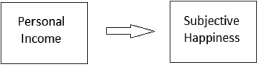
This model presents the efficient cause (personal happiness) as a source of change or production that precedes the effect (subjective happiness) in time. Although not relevant to material or formal cause, time is therefore critical when invoking efficient cause. Time is also relevant, but not necessary, to understanding final cause, which refers to a thing's end. When theorizing about persons, final cause can refer to the goals or purposes that explain behavior. For instance, a person enrolls in a psychology class to learn more about himself or herself, or enrolls in a Ph.D. program with the design of becoming a professor in the future. Final cause also entails natural end states as well that are important in explaining processes. For instance, the human body maintains a fairly steady overall temperature. When factors in the environment warm the body (efficient cause), such as when a Caucasian person sits in direct sunlight to deepen his tan (final cause), the body will change in ways to release the added heat (e.g., perspiration will increase; efficient cause), but it will not release too much heat in moving toward its balanced point (final cause). Another example involves growth; for instance, red oaks normally grow to approximately 90 feet whereas pinon pines normally grow to approximately 30 feet in height. These homoeostatic points or natural end states towards which things move or change are therefore also entailed in Aristotle's final cause (Wallace, 1996).
Biochemical pathway models are perhaps the simplest and most effective models to use when introducing students to Aristotle's four causes (e.g., an image of the Krebs cycle can be used: http://en.wikipedia.org/wiki/Citric_acid_cycle). The atoms in the model are the material causes, the structures of the different molecules in the model are the formal causes, the arrows in the model showing how compounds influence each other or change their patterns are the efficient causes, and the rhythmic, stable nature of the structures and processes in the model (viz., it is in a normal “holding pattern”) is the final cause. A simplified model of an atom can also be discussed. The protons, neutrons, and electrons are the material cause, the electrons moving about in time in their orbits are efficient causes. Students can also imagine energy being used to change the orbits of the electrons as an efficient cause. Formal cause is the “whatness” of the atom, it's pattern or configuration of matter that makes it to be a particular atom. Lastly, the structures and processes in the atom are in balance. Again, students can imagine adding or subtracting energy to change the orbits of the electrons, and in normal circumstances the electrons will settle into a stable holding pattern (final cause).
Once students appreciate the rich explanations of nature afforded by the four causes, they can apply them to psychological theories. A critical point must be made, however, either prior to or during this transition. The point is this: causes are bound to the natures of the things themselves. An unfortunate turn in history is that psychologists adopted a positivistic view of causation popularly found in the writings of J. S. Mill and David Hume. In this view, cause is reduced to efficient cause only, and moreover causes are regarded as consistent associations formed in the mind. In other words, the causal structure of nature itself cannot be known; rather, the consistent associations of sense impressions are all that can be known, and these consistently associated impressions are regarded as causation. This metaphysical standpoint not only reduces Aristotle's causality to Hume's causation, but it is highly subjective (viz., it fits with phenomenalism) as well and serves as the impetus for viewing the search for causes as largely a statistical exercise, as with mediation or structural equation modeling, or still worse solely as “equation surgery” (Pearl, 2009, p. 417). From the perspective of moderate realism, however, the search for causes is not necessarily statistical or mathematical and is instead similar to the sleuthing of Sherlock Holmes or Father Brown, requiring skills of careful observation, patience, right reasoning, and intuition to solve the mysteries of nature (cf., Freedman, 1991).
A simple mental exercise that will help students realize the distinction between Aristotle's causality and Hume's causation is to consider a scientist who develops a new type of fertilizer for corn. The scientist works with a computer program and with a molecular model kit to build models of the chemical compounds that will comprise the fertilizer. She then goes to the laboratory and manufactures the compounds and places a quantity of the fertilizer in a container. She writes instructions on the container detailing how the fertilizer is to be added to the soil to insure maximum plant growth and health. Next, consider a student working in the scientist's laboratory. Does the student need to know the molecular formulas for the compounds to test the fertilizer's efficacy on samples of corn crops? The answer is clearly, “no.” The student need only follow the instructions on the container to deliver the fertilizer in appropriate proportions to the samples. The student does not need to know the formal and material causal structure of the compounds. As the scientist begins working in her laboratory the causes exist intentionally in her mind. Once the fertilizer is created the causes inhere within it. The point is that causes are something more than simple Humean associations of sense impressions in the scientist's mind, they are instead “wrapped up” in the fertilizer's nature. This is what was meant above in stating that causes are bound to the natures of the things themselves.
Biochemical models, atomic models, computer models of the mind, and similar types of models used to understand the structures and processes of nature are referred to generally as analogical models (Haig, 2013); and when such models are developed to be faithful representations of specific natural systems (usually in visual form) they are referred to as iconic models (Harré, 1976). In Observation Oriented Modeling, these visual or diagrammatic models are referred to as integrated models to highlight the metaphysical position that nature is integrated and intelligible (i.e., explainable; see Doroughty, 2013). Perhaps the most challenging aspect of Observation Oriented Modeling, and the most challenging prospect for future psychologists as well, is the development of integrated (iconic) models. Examples can be found in Grice (2011) and Grice, Barrett, Schlimgen, and Abramson (2012), and students should be encouraged to develop such models on their own or as part of a common class exercise. It is most effective, however, to build a model for which actual observations (data) are available or can be obtained by the students. Students can collect data through an individual, approved project or through a common class project. Existing data can be provided by the instructor, requested from colleagues, obtained from open sources, or taken from printed material such as textbooks or instructional manuals. Integrated, iconic models are not widely used in psychology, hence the goal is to build such a model for the data.
An Exercise in Causal Modeling
Zealure Holcomb's (1997) Real Data workbook is an instance of an accessible resource for students that reports numerous studies with actual data. One example (p. 123) reports data for 135 women who visited a hospital seeking evaluation for self-identified symptoms of breast cancer, such as a lump or discharge (see Lauver & Youngran, 1995 for the original article). Among other things, the goal of the study was to identify the relationship between optimism and any delay in seeking the evaluation. The authors expected a negative linear relationship between the optimism and delay values as shown in the following variable-based model:

A negative relationship was expected partly because optimism has purportedly been shown to correlate positively with better future planning and with positive attitudes of acceptance (Lauver & Youngran, 1995, p. 203).
The optimism scores ranged from 0 to 4 and were computed from responses to the original Life Orientation Test, an 8-item self-report questionnaire. The women responded to statements such as “In uncertain times I usually expect the best” and “I'm always optimistic about my future” using a 5-point rating scale. The numerical ratings on the scale were then averaged. The delay values were also reported by the women and ranged from 1 to 2,538 days (i.e., days between initial detection of the symptom and the visit to the hospital). Over half of the delay values were less than 21 days, and several extreme cases were noted, which will be discussed below.
Students should be encouraged to write down their own thoughts and questions about the posited link between optimism and delay in visiting a doctor. The following types of questions may emerge:
“Are optimistic women necessarily better planners, and why isn't planning in the model?”
“Once an optimistic woman has identified what she thinks is a cancerous lump, would she necessarily feel a sense of panic and want to immediately see a doctor, or would she be less worried?”
“Wouldn't an optimistic woman actually be more likely to judge the lump as non-cancerous and therefore delay a visit to the doctor?”
The last question would in fact lead to an opposite expected correlation, but the more general and important point is that the students' questions will likely not fit any variable-based model and Pearson correlation analysis. Why? Because to be perfectly consistent, models like the one above only permit statements about variables, such as “Relatively high values on the optimism scale are expected to be associated with lower reported delay values,” or “Optimism scores are expected to be negatively correlated with delay values (estimated r = −.20).” Again, compare these statements carefully to the ways students will naturally think about the problem. When thinking about optimists and the time it takes them to report to the doctor the students' natural focus is on the persons in the study, which is proper for discussing causes that firstly inhere in the women themselves, not in the variables and variable labels (e.g., “optimism”) constructed by the researchers. This statement is of course in line with philosophical realism, and the capability of creating consistency between how students will think naturally about the world and how they will analyze their observations is one of the main advantages of Observation Oriented Modeling and the OOM software.
By focusing on the persons in the study, the integrated whole under consideration by the students is any given woman detecting an anomaly in her breast. The integrated model (a type of iconic model) therefore begins with a person, as shown in Fig. 1. In this case, a simple stick figure is drawn to represent an individual woman in the study. Every integrated model must begin with a judgment about the integrated whole or the system under investigation, whether it be a person, a baseball team, another type of animal, an atom, a bio-chemical process, etc. As shown in Fig. 1, a mind-body distinction is made by denoting that the woman senses the lump in her breast, presumably by using her hands and fingers. In her mind an abstraction is made on the basis of what is reported by the senses. This abstraction is denoted in the figure by the circle enclosing the word “lump” and a picture of the lump. How abstraction occurs and whether or not it includes a visual component is not spelled out by the model in its current form. The woman must, however, know that her fingers have detected an internal lump rather than, for instance, an external skin tag.
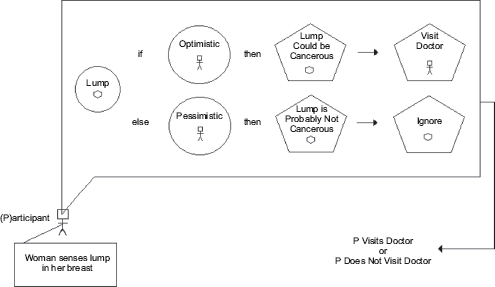
Integrated model for optimism as a cause of planning a visit to the doctor.
With the lump identified, the model next incorporates optimism, and the question is raised, “What is optimism?” On the one hand, it may be considered a quality inhering in the woman and may therefore be subject to observation by another person. On the other hand, the actual observations relevant to optimism in the study are self-report. It is more appropriate, therefore, to represent optimism as an abstraction made by the woman. Similar to “this is a lump,” the abstraction is “this (myself) is a pessimist.” The problem with this part of the model, however, is that it does not fit the optimism observations which are numbers computed by averaging values attached to a scale for judgments about the self (e.g., “I'm always optimistic about my future” rated on a scale with values from 0 to 4). With scores ranging from 0 to 4, is it presumed that optimism is a continuum? Moreover, is it presumed that the woman somehow erects a crude “optimism ruler” in her mind upon which she demarcates herself? How would such a process actually occur? By contrast, why cannot one statement, such as “Generally speaking, I consider myself to be an optimist,” be used and code it as “Yes” or “No?” Why use a 5-point scale (0 to 4) rather than a 9-point scale? Does averaging items somehow improve the scores? Students can be encouraged to ask additional questions about the questionnaire in an attempt to determine what the optimism values actually mean in the context of the nature of optimism itself. They will quickly realize that theoretical, not statistical, answers are required, and they will learn that making relevant observations about optimism requires a richer theoretical understanding of exactly what it is as a quality ostensibly inhering in persons.
Proceeding with the example, nonetheless, and presuming that optimism is an abstraction drawn from the sensory and intellectual “data” of one's self, it is logically related to judgments about the lump discovered in the breast. If the woman forms an abstraction of herself as optimistic, then she will judge the lump as cancerous; whereas if she forms an abstraction of herself as pessimistic, then she will judge the lump as not cancerous. A judgment is distinguished from an abstraction by representing the former as a regular pentagon (see Fig. 1), and again exactly how the woman makes a judgment is not spelled out by the model. Once either judgment is made, then it acts as an efficient cause (arrows in the model) for a judgment regarding whether a visit to the doctor is warranted or the lump can be ignored. It can be seen in the model, however, that the lump is judged as “could be” or “is probably not” cancerous. Are these the expected judgments? Would it be an important difference if the woman judged the lump as “most certainly cancerous” or “absolutely not” cancerous? Would such judgments be an effect of optimism or some other judgment about oneself, such as fatalism? Students may also ponder if, as suggested above and contrary to the study authors' expectations, the pessimistic woman should actually be the one who judges the lump as cancerous and who rushes to make an appointment with her doctor; after all, bad things like cancer are expected to happen. All of this is left open to debate for the students, because the point is that the integrated model in Fig. 1 is much more rich and complex than the simple variable-based model above. Asking students to construct an integrated model will require them to think about the structures and processes under investigation; in other words, to think in terms of causality rather than simply causation.
Finally, outside of the woman's mind in the model, whether or not she visited the doctor is observed. Again, to be truer to the observations in hand, the model needs to be adjusted so that the number of days between detecting the anomaly and the first visit to the doctor is the “output” from the internal features of the model. Whether the structures and processes are directly observable or not, the observations acquired must reflect some commitment to them, which is partly why this overall approach is referred to as Observation Oriented Modeling.
From Statistics and Aggregates to Patterns and Individuals
As Fig. 1 shows, the proper level of reasoning about causes and effects is at the level of the individual women in the breast cancer study. If the causal model is accurate, then a woman who self-identifies as an optimist should not delay in seeking an evaluation from a doctor, and a woman who self-identifies as a pessimist should delay seeking an evaluation. The actual data from this study were obtained, however, under the phenomenalism (see Table 1) inherent in the variable-based model shown above. Some ambiguity or difficulty must therefore be expected when attempting to analyze the data with the OOM software (Grice, 2011). Nonetheless, students will learn important lessons when they attempt to analyze the data from the breast cancer study. 3
An Initial Exercise in OOM Data Analysis
In the variable-based model, optimism and delay were assumed to be continuous quantities, hence a Pearson's correlation was computed and reported by the study authors. The correlation was significant (r = −.18, p < .05, two-tailed). It is also important to point out that the authors transformed the delay responses due to radical skewness and a number of salient outliers. The p value of course indicates that, assuming the null hypothesis is true, and a host of other assumptions have been met (including random sampling, bivariate normality, and homoscedasticity), the probability of obtaining results as extreme or more extreme than −.18 or .18 is less than .05. The conclusion to be drawn in the standard null hypothesis significance testing procedure is therefore that the two assumed continuous variables are linearly related in the population. The observed correlation serves as the estimated magnitude of the linear association, and at −.18 is rather anemic.
In the OOM software, students must first define the units of observation for the optimism and delay values. Rather than refer to optimism and delay as variables, in OOM they are referred to as “orderings” to reflect the understanding that nature is integrated and ordered in particular ways. The integrated model is supposed to reflect this ordering, both in terms of how the optimism and delay observations are ordered or structured within themselves and how they are ordered to one another. As derived by the study authors, the optimism observations are ordered into 33 units (0, 0.125, 0.250, 0.375,… 3.875, 4.00). Recall these values were computed by averaging responses on a 0–4 scale to eight items on the Life Orientation Test questionnaire. A simpler less precise ordering should be used to make the task of building and testing a pattern, as described below, more manageable for students. Twenty units work well, with scores ordered as 0–0.20, 0.21–0.40, 0.41–0.60,… 3.81–4.0. The delay observations can similarly be ordered into 20 units as shown in Fig. 2. The task here is similar to creating a grouped frequency histogram, but the overall goal is to build a model for explaining how the optimism and delay observations are to be ordered to one another. The groupings into units here is entirely ad hoc, whereas in original research how the observations are ordered will be determined by an integrated model.

Delay and optimism observations grouped into 20 units. Each asterisk indicates two persons, and observed frequencies are reported in square brackets.
With the observations grouped into their respective units, the next goal for the students is to devise a way of ordering one set of observations to the other, and the simplest and most powerful way to introduce them to this idea is through the Pattern Analysis – Crossed Observations procedure of the OOM software. By crossing the two orderings a matrix is created, as shown in Fig. 3. The question now is, if the optimism observations represent the cause, and the delay observations represent the effect, how are the effect observations ordered to (or conformed to) the cause observations? In simpler terms, what is the expected cause-effect pattern? Here the students are working visually rather than with equations, although simple equations could be used to determine a predicted pattern for discrete or continuous values. Figure 3a shows a pattern the students might suggest. The units are matched, in order, on a one-to-one basis with units ostensibly representing high optimism matched with units representing short delays in choosing to visit the doctor. Every woman in the study is expected to be found in one of the grey squares denoted in the pattern. The students can be further pressed to explain exactly why the observations (all of the women) should fall exactly in the grey units of the pattern. They may wish to build some imprecision or “wiggle room” into the expected pattern, like that shown in Fig. 3b, or they may opt for a more radical dichotomizing as shown in Fig. 3c. As debate ensues, students should be encouraged to return to the integrated model, which will again require them to take greater responsibility in thinking clearly and deeply about optimism itself (what it is, and how it must be observed) and exactly how it affects a decision to seek evaluation for an anomaly in the breast.

Expected patterns (darkened cells) for optimism and delay orderings (a–c), and actual observations for 135 women (d).
Using the imprecise pattern in Fig. 3b, the OOM software has an option for showing the observations in the figure as well. As can be seen in Fig. 3d, only about one quarter of the observations fit the expected pattern. With such a simple and elegant visual tool the students immediately realize using only an “eye test” that the prediction is a bust. Of the 135 women, only 33 observations (24.44%) were located in the expected crossed units. Without any equations, without any p values, without any statistical assumptions, and without any attempt to conjure an imaginary population, the students are also here reminded of the importance of accuracy in science. The current cause-effect pattern is clearly inaccurate, and since the pattern is derived from the integrated model developed by the students, the integrated model is deemed inaccurate as well. This is the primary question to be answered in Observation Oriented Modeling: Is the model accurate? As an intentional representation of the causes and effects inhering in the women in the current example study, the model is largely a failure.
Beyond the simple and elegant graph, the OOM software provides summary information regarding the accuracy of the model.

The Percent Correct Classification (PCC) index, as noted, is only 24.44%, and this is the primary numeric result to be considered. The PCC index is computed or derived for most all of the analyses available in the OOM software, and students should be encouraged to look for it first in the program's output. As can also be seen, a probability statistic can be requested and used in an entirely secondary role. This probability statistic is referred to as a chance value, or c-value, in OOM in order to avoid confusion with the p value commonly encountered in null hypothesis significance testing. The c-value is in most instances in OOM derived from a randomization test, which is becoming more widely recognized by quantitative experts as superior to traditional p values (see Manly, 2006; Howell, 2007, Chapter 18) despite being lauded as early as 1969 (Winch & Campbell).
The c-value for the breast cancer data is computed by randomly pairing the optimism observations with the delay observations. Specifically, the optimism values for the 135 women are randomly shuffled. The predicted pattern is then applied to the randomly paired optimism and delay observations and the PCC index computed. If this PCC index equals or exceeds the PCC index for the actual data (here, 24.44), then randomized data performed just as well as the actual data in the context of the model, which is not a desirable occurrence. This process of randomizing the data and comparing PCC indices is repeated a set number of times (1000 trials in the output above) and the results tallied. The c-value is the proportion of instances in which the PCC index from the randomized data equaled or exceeded the PCC index for the actual data. As with the traditional p value, then, a low value is desirable, although no rational person would put forth or adopt a universal convention to determine “significance” (e.g., c < .05). The c-value is entirely secondary, whereas the integrated model and PCC index are primary. The c-value in the shown output for the breast cancer data is .35, indicating that for 355 of the 1000 trials, a PCC index of 24.44 or higher could be achieved by simply randomly shuffling the data. Not only is the PCC value of 24.44 unimpressive, but it is fairly ordinary or usual as well.
Lastly, in the move from aggregates to persons, students can be asked to compare their interpretation of the PCC index to the Pearson's correlation coefficient. Recall the correlation between optimism and delay for the breast cancer data was −.18. Students can be challenged to interpret the correlation coefficient in a way that can be applied to the 135 women or to any given woman in the study. The correlation can be squared as well to convert it to a proportional statistic. Again, students can be challenged to explain how accounting for 3% of the variance in one variable by the second variable applies to the 135 women or any given woman in the study. The point of asking students to interpret the correlation in this way is of course to remind them that their interpretation must be confined to the variables; i.e., the variances and covariances of the variables. There is simply no clear way to cross the bridge from the aggregate statistic (the Pearson's r) to the scores, or observations, themselves in a way that conveys the meaningfulness of the result for these women. By contrast, the PCC index is tied directly to the observations and how they are ordered, both in terms of their units and in terms of the expected pattern. Whether or not any given woman's observations are consistent with the integrated model and pattern analysis can be determined. Indeed, using options in the OOM software students can explicitly identify the 17 women whose observations fit the expected pattern. The readily interpretable PCC index can also be compared to the correlation value in this example to remind students that “statistical significance” does not indicate practical, clinical, or theoretical significance (Thompson, 2002), nor does statistical significance indicate that even a simple majority of observations fit an hypothesized model. Lastly, students can contrast this rich exercise of thinking about what the scores on the Life Orientation Test really mean and how they are causally related to observations of delay, with the relatively sterile exercise of checking statistical assumptions and interpreting the magnitude of the observed correlation coefficient according to some arbitrary convention (e.g., “according to Cohen's conventions, a correlation of −.18 represents a small effect size”).
From Effect Sizes, p-values, and Parameters to Accuracy, c-values, and Chance
From the perspective of Observation Oriented Modeling, the word “effect” has been hijacked by phenomenalism (see Table 1), or more specifically by statisticism (Lamiell, 2013). Because psychology has primarily adopted statistics, particularly null hypothesis significance testing, as its main approach to working with quantities (discrete or continuous), the word “effect” has taken on an esoteric meaning not generally understood by scientists, philosophers, or the general public. The word and its derivatives are of course powerful and influential, as can be seen in statements such as: “The effect of the SAD light in combating depression was significant,” “The effectiveness of the psychoanalytic treatment was negligible,” “The bystander effect is reliable,” “This effect has been observed across numerous studies,” and “The size of the effect was rather large.” These statements convey a sense of importance, certitude, and scientific understanding, even though no details of the studies from which they may have come are provided. The meaning of effect in modern psychology, however, typically has very little to do with certitude and is instead almost always embedded in a probabilistic or statistical point of view.
An introductory class exercise regarding the meaning of the word “effect” requires students to write about any event in their lives and then explain why the event happened. Students may respond: “My car wouldn't start today because the battery was dead,” “I felt sick last week because I contracted the flu from my brother,” “My girlfriend and I broke up because we discovered we have little in common.” Normally, the students' statements will attribute a cause to each event and will express an understanding of nature that seems to run deep while also transcending the particular events of their lives. Such thoughts express the way things truly are…the way nature is. Cars with dead batteries don't start, people who contract the influenza virus grow ill, and uncommon people cannot stay romantically tied for life. But are these statements true? Do they really express the way nature is? Cannot an old car without electronics be physically pushed and started by popping the clutch? Aren't some people immune to certain strains of influenza? With respect to romantic relationships, is it not also true that sometimes “opposites attract?” Clearly, gaining an understanding of nature will require more than the students' day-to-day informal thoughts of causes and effects. Still, each question raised implies that an answer might be found, thus bringing students to the doorstep of science; for as Aristotle understood well, the business of science is causal explanation.
With a statement such as “The effect of the SAD light in combating depression was significant,” the psychologist is also intending to express a causal relation; namely, the SAD light causes a reduction in depression. Such statements are the “stuff” of science, but in psychology these causal-sounding expressions are almost invariably statistical expressions. While students may naturally pair effects to their causes in the class exercise described above, in psychology the opposite of “effect” is not typically “cause” but rather “null statistical difference.” In other words, an effect is said to be found when the null hypothesis has been rejected; in other the words, an effect is a statistically significant finding. The magnitude of the effect or the size of the effect moreover often refers to the average difference between groups or the proportion of variance shared by two variables. A useful exercise to drive home these points is to again rely on published data, contrived data, or data from workbooks or textbooks. These data can be used “as is” or manipulated in a way to shed light on what is meant by a statistical effect.
An Exercise on Effect Sizes in the OOM Software
In his chapter on t tests, David C. Howell (2007) reports an example data set of weight gain (or loss) for anorexic girls who received therapy for their eating disorder and those who did not receive therapy. The outcome variable is the amount of weight gain, in pounds, from the beginning to the end of the treatment or therapy. In the parlance of modern research design, the grouping variable (Therapy vs Control) is the independent variable and cause, while weight gain is the dependent variable and effect. Using a standard variable-based model, the relationship between the two variables can be shown as follows:

Howell's original data were altered here so that the computed effect size would be medium according to popular conventions and in the expected direction (i.e., the mean for the Therapy group will be greater than the mean for the Control group); yet, when examined at the level of the individuals, most anorexic women would actually keep their existing weight or lose weight, contrary to prediction. The altered data are reported in Table 2, and the exercise to be performed by students is to analyze the data using the traditional null hypothesis significance testing approach and the OOM software.
Weight Gain Data, Example Data, and Randomized Data For Control and Anorexia Therapy Groups

Weight is a continuous quantity, and the observations are independent both between and within groups. An independent samples t test is therefore suitable for these data, and the hypotheses can be written in three-valued logic form (Harris, 1997),

The μ's of course represent population weights in pounds. Students will find that the Therapy group gained an average of 1.35 pounds (SD = 3.72) compared to the Control group who lost an average of 1.23 pounds (SD = 3.25), thus supporting the predicted difference (95%CI = 0.77 ≤ μT – μC ≤ 4.38) and efficacy of the therapy. The t test is statistically significant (t58 = 2.86, p = .006), at the .05 level, and the magnitude of the effect (d = 0.74, η2 = 0.12) is nearly large according to Cohen's widely used conventions (d = 0.80 is a large effect). Examination of the data also reveals no salient outliers, but the distributions appear to be somewhat bimodal, particularly for the therapy group, when examined with histograms. Boxplots, however, will show only moderate skewness.
Students should be required to list and evaluate or discuss the various assumptions of the independent samples t test: (1) random sampling or random assignment to groups, (2) continuous dependent variable, (3) null hypothesis is true, (4) p ≤ .05 is a reasonable cut-point for statistical significance, (5) normal population distributions, (6) observations are independent both within and between groups, and (7) homogeneity of population variances. Many of these assumptions of course underlie the validity of the observed p value, a probability the students should be expected to understand completely. An excellent resource for checking students' understanding of the p value is Oakes' (1986; see also, Gigerenzer, 2004) 6-item quiz. In the context of discussing the p value students should also be challenged to define the populations under consideration. Are they all women? Are they women from certain ethnic groups or regions? Are they women of certain ages? Are they women now living, or do the populations include women from the past and future? The point of this challenge is to remind students that psychologists are almost always working with arbitrarily defined, imaginary populations. The population means are therefore almost always non-empirical; i.e., they are values that cannot be obtained in actuality. The essential lesson to be learned from discussing assumptions and populations is that null hypothesis significance testing is an extremely abstract, mathematical-statistical routine in which the primary goal is to pursue (estimate) population parameters that rarely have any basis in lived reality.
Turning to effect size, by declaring the t test “statistically significant” and rejecting the null hypothesis, the conclusion is that the population means differ by some magnitude. Cohen's d represents a standardized estimate of that magnitude based on the sample means and pooled standard deviation. For the current data the value is computed as,

The formula incorporates aggregate statistics and consequently has no direct bearing on any one of the women in the study or on any pair of women from the two groups. As has been made abundantly clear above, however, causes and their effects inhere in the things or entities under investigation – in this instance, the women in the two groups. Students should be challenged to relate the value of d to the women in the study. Another popular index of effect size is η2, which the students should compute and again attempt to relate to the women in the study: η2 = t2/(t2 + df) = 2.862/ (2.862 + 58) = 0.12. This task will prove even more difficult as the interpretation of η2 is one based on shared overlap between variables. The value of 0.12 indicates that the independent and dependent variables share 12% of their variance. Conveying what this effect size index means for the actual effectiveness of the therapy for the individual women in the study is impossible, which is why psychologists eschew the problem by using Cohen's arbitrary conventions to describe their effects as small, medium, or large.
By contrast, analyzing the same data in the OOM software will remind students that causes inhere in the persons in the study, and that any discussion of effects must be relevant to these persons. The analysis begins by first defining the units of observation. The women are observed to be in one of two groups: the Therapy group or the Control group. These two units of observation represent the cause, or they at least carry information about the causal forces effecting weight gain or loss (in Observation Oriented Modeling, an integrated model must eventually be worked out to truly understand the causes). The changes in weight are continuous quantities representing a change in this quality (heaviness) over time. The values in Table 2 range from −7.5 to 7.5 pounds for the two groups of women, and most of the women have unique values. In OOM, continuous quantities must often be grouped so that each unit (value) is represented by more than one observation. Because a population parameter is not being estimated, the notion of statistical power is meaningless in OOM. Observations can consequently be grouped without fear of losing power. While modern methodologists, for instance, advise strongly against dichotomizing data (MacCallum, Zhang, Preacher, & Rucker, 2002; Irwin & McClelland, 2003), such alterations are welcome in OOM if they advance the goal of identifying clear and meaningful patterns in the observations. The weights for the two groups of women were thus organized into 8 units (–8.0 to −6.1, −6.0 to −4.1,… 4.0 to 5.9, 6.0 to 8.1). Students can be encouraged to try different groupings after the initial analysis and explore how they affect the results, as will be shown below.
The Build/Test Model option in the OOM software is then used to attempt to bring the 8-unit weight ordered observations into conformity with the 2-unit group ordered observations using binary Procrustes rotation, a procedure that does not rely on means or covariances but is instead based on the observations themselves (see Grice, 2011, Chapter 3). The analysis is ad hoc compared to the a priori pattern defining methods used with the breast cancer data above. Specifically, the algorithm examines the relative magnitudes of frequencies of observations and determines how every observation should be classified based on the predominant pattern in the data. Each observation is then evaluated according to this pattern and judged as either correctly or incorrectly classified. The results can be presented in a simple graph referred to as a “multigram.” To help students interpret multigrams, instructors should prepare at least two contrived sets of observations, like those reported in Table 2, showing clear patterns. Consider 60 weight observations, for instance, in which all of the women in therapy gain two or more pounds while all women in the control group lose weight or maintain their current weight (column labeled “Clear One” in Table 2). The resulting multigram is shown in Fig. 4. As can be seen, a multigram graphs the two frequency distributions side by side, and in this extreme example the two distributions do not overlap at all. A clear pattern is present in which the weight values can be separated into two groups. The Percent Correct Classification (PCC) index for these data is 100%, and the pattern clearly supports the effectiveness of the therapy. Every woman in the therapy group gained weight, and moreover gained more weight than every woman in the control group.

Multigram of clear pattern example. This pattern matches expectation with the individuals in the Therapy group gaining weight.
As another extreme example, consider data (“Clear Two” in Table 2) that generate the multigram in Fig. 5. Again, the 8-unit weight observations can be classified into the 2-unit group orderings with remarkable accuracy (PCC = 96.67%). The pattern in the multigram shows that: (1) all of the women who gained 2 or more pounds were in the Therapy group; (2) all who gained up to 1.9 pounds or lost as much as 6 pounds were in the Control group; and (3) most of the women who lost 6.1 or more pounds were in the Therapy group, contrary to expectation. Based on the relative frequencies both within the 8 weight units and the 2 group units, the algorithm determined that all of the observations should have fit this pattern and were therefore classified as such. As can be seen in Fig. 5, then, two observations (viz., two Control women who lost 6.1 or more pounds) were inconsistent with this overall pattern and were hence counted as misclassified by the algorithm even though they were in the Control group and lost relatively large amounts of weight. This example thus demonstrates that the algorithm works on the pattern of observations (data), not on the researcher's predicted pattern of results as in the breast cancer study above. Nine women in the Therapy group lost 6.1 or more pounds, which is entirely contrary to expectation; yet, the algorithm counted them as correctly classified. Only two women in the Control group lost this much weight, and all of the other women in the Therapy group lost more weight than all of the women in the Control group. Based on the clear separation between groups of observations, the algorithm determined that all women who lost 6.1 pounds or more should be classified as belonging to the Therapy group, which unfortunately contradicts expectation. The analysis is entirely ad hoc, however, making such outcomes possible. A high PCC index in the Build/Test Model analysis therefore only indicates that the observations formed a clear pattern. It does not mean that the pattern fits the scientist's expectation. The multigram must be examined – preferably in light of an integrated model – to decide whether the pattern is consistent with expectation or theory, and students will quickly realize that interpreting the effects (and causes) embodied in a multigram is clearly different from computing and interpreting statistical effects embodied in d and η2.

Multigram of clear pattern example. This pattern does not match expectation perfectly, as nine women in the Therapy group lost weight. These nine women were classified as correct by the ad hoc algorithm used in the analysis because they were distinct from the other observations.
The extreme multigrams and their accompanying data in Table 2 can also be used to help students understand the chance value. Specifically, each student can be asked to shuffle randomly the weight change values (“Clear One” in Table 2) that generated the multigram in Fig. 4. Values can simply be changed in the OOM software, making certain the students randomize a large number of the 60 values across both groups. In this way, some weights for the women in the Therapy group will be given to women in the Control group and vice versa. Once the weights are randomly shuffled, the students run the binary Procrustes rotation and examine the multigram and PCC index. Fig. 6 shows an example multigram from the randomized data (labeled “Random”) in Table 2. The clear pattern in Fig. 4 has now been lost, and the PCC index for the randomized data, 61.67, is much smaller than the PCC index for the “Clear One” data (100%). The randomization test in OOM simply repeats this process a set number of times (e.g., 1000 trials) and determines the proportion of trials in which the PCC index equals or exceeds the original value. This proportion is the chance value, or c-value, and for the data in Figs. 4 and 5 it is less than .001, indicating that not one time in 1000 trials did the randomized data yield PCC indices as high as 100 or 96.67, respectively. A low c-value indicates that randomized versions of the observations do not readily produce a pattern as clear or discriminating as the one obtained for the actual data. It informs the students of the distinctiveness or unusualness of the observed PCC index and accompanying pattern, and it does so without any assumptions. Recall from above the list of assumptions necessary for the accuracy of the p value for the independent samples t test (e.g., normality of population distributions, homogeneous population variances, independence of observations). None of these assumptions are required for the randomization test (Manly, 2006), and students will consequently find the c-value to be concrete, simple, and intuitive in comparison to the traditional p value.

Multigram of randomized data with no clear pattern.
Turning students to the OOM results for the actual weight data in Table 2, the multigram in Fig. 7 reveals that a single discrimination point between the two frequency distributions cannot be made. Nonetheless, a pattern of bimodal, non-overlapping units is evident in the multigram, permitting a large number of the observations to be correctly and distinctively classified, PCC = 86.67, c-value < .001. The OOM results are as follows:

Multigram of weight gain data for Control and Therapy groups. This pattern partly matches expectation, but 11 women in the anorexia Therapy group lost weight and were classified correctly by the ad hoc algorithm because of their distinctiveness.

The OOM software has detected a pattern that classifies an overwhelming majority of the women correctly based on the observations themselves…but what is the meaning of the result? Because population parameters are not estimated, the three-valued logic hypotheses above are not relevant. Without an integrated model to guide their thinking, students must examine the multigram in Fig. 7 and interpret the pattern. As can be seen, it appears the effect of the therapy is dichotomous. Sixteen women have lost weight, which is a terrible outcome given they are anorexic, while 14 women have gained weight, which is a positive outcome. The Control group as well appears to be made up of two groups, those who lost approximately 1 to 8 pounds and those who gained approximately 1 to 4 pounds. Cohen's d and η2 offered no information about these patterns, and to speak of d as indicating a “typical” standardized difference between women in the two groups is recognized as misleading. A majority of women in the Therapy group actually lost weight, contradicting the t test conclusion supportive of the efficacy of the therapy – a disaster for the anorexia therapy.
If the weight observations are represented as two units (–0.1 to −8.0, weight loss; 0.1 to 8.0, weight gain), then the meaning of the results for the women in the study becomes even more clear. As can be seen in the multigram in Fig. 8, the two groups of women appear highly similar with respect to the 2-unit weight observations; and again, a small majority of women in the anorexia therapy group actually lost weight. These 16 women in the Therapy group were therefore classified correctly by the algorithm, a result entirely opposite of expectation. This analysis also shows, however, no ability to discriminate clearly between the women in terms of simple gain or loss in weight, as indicated by a PCC index of 51.67 and c-value of 1. In every instance, randomized versions of the data yielded a PCC index of 51.67 or higher, indicating that the pattern in Fig. 8, although opposite of expectation, is not at all distinct.
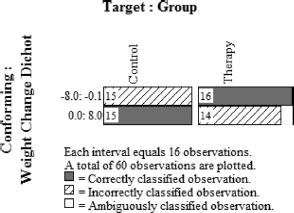
Multigram of weight gain data for Control and Therapy groups. Weight gain has been ordered into two units, and the pattern is opposite of expectation with a slight majority of women in the anorexia Therapy group having lost weight.
Effect size indices accompanying results for most modern statistical analyses are understood to be aggregate-based or variable-based values that are difficult to interpret without the aid of established conventions, like Cohen's conventions. As such, they are not effects that are logically tied to the causes that inhere in the people in the study. Effect sizes are statistical, aggregate summaries of the data, and their magnitudes have no meaning for any given individual in the study. Through this particular class exercise, students realize that OOM analyses are not based on aggregate statistics. Not a single mean, median, or standard deviation has been invoked. The output across analyses is also highly similar, allowing students to focus on the primary information; viz., the patterns and PCC indices. This streamlining is possible because OOM reduces all data to a common binary form, referred to as deep structure, upon which the analyses are based. Moreover, the goal in OOM is not to estimate abstract population parameters, but to accurately classify the observations based on some a priori or ad hoc pattern (ideally, of course, an integrated model would be available for explaining the pattern). Accuracy is therefore the key judgment, and the PCC index is readily understood by students, other scientists, and laypersons as well. The c-value in OOM is also free of assumptions and relatively concrete compared to the traditional p value in null hypothesis significance testing, and is based on a firm foundation of reasoning dating to at least the 1960s (Winch & Campbell, 1969). Nonetheless, the inference to cause and effect is only aided by a high PCC index and low c-value. The basis and force of such an inference ultimately rest upon the structures and processes in an integrated model.
From Continuities and Variables to Entities and Their Qualities
With regard to measurement, one of the three domains of quantitative training reviewed by Aiken, et al. (2008), students of psychology are universally taught to memorize and apply Stevens' (1946) four scales of measurement: nominal, ordinal, interval, and ratio. They are also taught to select their statistical analysis procedures based upon this classification scheme, and to regard parametric statistical methods for interval and ratio measurement as more powerful – statistically speaking – than nonparametric methods. What students are rarely taught, however, is that Stevens' view is a product of phenomenalism (see Table 1) and that he invented his scales of measurement in direct response to charges that psychologists had not demonstrated true measurement of the qualities they were studying (e.g., sound perception, intelligence, personality traits, depression). More specifically, psychologists had not successfully established units of measure with clear additive properties for any of the qualities.
While it can be intimidating, this history is important to present to undergraduate students. Michell's (2011) ghost of Pythagoras paper provides an excellent overview, Grice (2011, p. 145–150) presents an example in which an attempt is made to measure intelligence with reaction time, and Sherry (2011) recounts the history of measuring temperature. Another avenue for introducing students to the pitfalls of modern methods of measurement is to build upon the pitfalls of aggregating data, as shown above with the anorexia therapy example. That example revealed how interpreting results based on aggregate statistics can be difficult and misleading. The same principle holds true when aggregating responses across items, as is done in so much of psychological research today. An exercise to demonstrate this point includes the development of a fictitious “Need for Speed” questionnaire.
An Exercise in “Measurement”
Following modern psychometric theory, students are instructed at the beginning of this exercise that Need for Speed is a continuous latent variable that cannot be measured without error. More or less time can be spent on discussing the modern conceptualization of latent variables (e.g., see Bollen, 2002; Borsboom, 2008), but the pragmatic point is that multiple items must be constructed from which scores (values) can be obtained. These scores are expected to vary from person to person for two reasons: (1) variation due to true individual differences in Need for Speed, and (2) variation due to unknown factors (errors). The latter errors are often undifferentiated and expected to be normally distributed and independent. This is of course the simple classical true score model of psychometrics.
Eight items are written to include in the questionnaire, as shown in Fig. 9. Data are obtained from ratings on a Likert-type scale, i.e., arbitrarily numbered with values from 0 (highly disagree) to 6 (highly agree). The fictitious data for this exercise are reported in the Appendix. Students next conduct a standard item analysis, examining the inter-item correlations, corrected item-total correlations, and Cronbach's α. The results from this analysis will show that all pairs of items are positively correlated, and the corrected item-total correlations are all positive and greater than .45. Cronbach's α is also impressive, with a value of .83. Based on these results, the scale is said to be reliable with respect to internal consistency. Advanced students can also be required to factor analyze the data, the results of which will reveal a strong single factor on which each of the eight items loads positively (minimum loading = .58). Based on these results, the scale is said to possess some construct validity as it is judged to be unidimensional, which is consistent with the understanding of Need for Speed as a single, continuous latent variable.

Hypothetical Need for Speed questionnaire.
With sufficient reliability and evidence for a single dimension, students are taught to sum the item responses to generate a scale score that is allegedly more reliable and valid than any of the individual eight items. Advanced students can discuss the pros and cons of computing more complicated factor scores based on the results of the factor analysis. For the analyses below, however, simple sum scores will be used. Finally, as a segue to concurrent validity and perhaps multi-trait multi-method matrices, students can compare men and women (data are provided in the Appendix) on the Need for Speed sum scores using traditional statistics. The results for an independent samples t test are statistically significant at the .05 level (t78 = 2.11, p = .038), with a medium effect size (d = 0.47, η2 = 0.05) and relatively precise 95% confidence interval (0.21 ≤ μ1 – μ2 ≤7.04). As might be expected, the mean for men (M = 29.08, SD = 6.87) is higher than the mean for women (M = 25.45, SD = 8.40).
Having worked through these psychometric and statistical exercises, students are then challenged to critically examine their work and to transition to new ways of thinking. The first step is to ask students, “What exactly is Need for Speed?” Is it a less reasonable construct to investigate than depression, intelligence, need for cognition, perfectionism, gender, etc.? If it exists in human nature, exactly how does it exist? Is it reasonable to consider it to be a continuous dimension along which people can be measured in extremely precise units…even in theory? When discussing Need for Speed at this level, it is important to help students distinguish between qualities, things, and variables. A quality, speaking generally in the context of psychology, is something that exists within persons. When a student walks into a classroom, he or she recognizes various things, some of which are fellow students and some of which are objects used for instruction (tables, desks, marker boards, etc.). By differentiating between persons and objects, the student understands the substantial form, or “whatness,” of the things in the room. The student of course also realizes that some students are shorter than others; some have brown hair while others have black hair; some are more vocal than others, while others seem more reserved; and so on. These recognized differences inhere in the persons themselves and do not exist in and of themselves. They are what philosophical realists would refer to as “accidents.” In other words, a student walking into the classroom does not see “hair color,” “height,” “shyness,” etc. as things; rather, he or she sees fellow students who possess these qualities. The student sees Lisa who has black hair and Jeremy who has blond hair but never “hair color” as a thing or substantial form.
A variable is not a quality; rather, a variable is a product of human reason, as when a student states, “Let x equal scores on the Need for Speed questionnaire, and y equal measured height.” A variable is therefore a product of the human mind (subject) engaged with things and their qualities (substantial forms and accidents). Variables of course play an important role in science by providing formal representations of things and qualities that can be manipulated by reason alone. The important point being made here, however, is that the subject-object dialectic is important in philosophical realism and must be maintained. Too often statisticians and psychologists fall unintentionally into phenomenalism, which then creates a propitious context for remaining trapped in the abstract world of null hypothesis significance testing. Consider, e.g., David Howell's definition of variable in his excellent statistics textbook, “A variable is a property of an object or event that can take on different values” (2007, p. 3). This definition unfortunately conflates and confuses qualities (referred to as “properties”) that exist in the persons or objects of study, and variables that exist in the minds of the investigators.
While they certainly have not been without controversy over the centuries, Aristotle's ten categories of being may help students think more clearly about their research and about Need for Speed in the current exercise. The categories are listed, defined, and exemplified in Table 3 for a student named Sandy who completed the Need for Speed questionnaire in August of 2013 in the Personality Research Laboratory at Oklahoma State University (see Wallace, 1977; Studtmann, 2007). Examining the list, students will most likely regard Need for Speed as a quality, particularly a habit, which for Aristotle was an enduring tendency to act in certain ways to consistently achieve a particular type of end. A virtue such as justice, e.g., can be said to be a habit if the choices and actions of a person repeatedly result in right and just outcomes. Need for Speed may similarly be thought of as such a tendency. The great difficulty over the centuries, however, has been whether or not some qualities are “rooted in quantity” (Wallace, 1977, p. 30). The rulerlike appearance of the Likert-type scale with its numbered values and the sum scores for the Need for Speed questionnaire suggest the quality can be understood as a continuous quantity; what St. Thomas Aquinas referred to as a “quantitative quality” or quantitas virtutis (see Crowley, 1996; Grice, 2011, Chapter 8; Echavarría, 2013). Absolutely no evidence, however, has been presented to support this claim. The students may appeal to the excellent results from the item analysis and factor analysis of the Need for Speed questionnaire, but as Michell (1999, 2008, 2011) has made clear, these analyses (and structural equation and item response models as well) assume continuous quantities, they do not provide evidence for quantitative structure.
Aristotle's Ten Categories of Being

An effective way to prompt students to think critically about the continuity assumption, and indeed the assumptions of the classical true score model of psychometrics, is to consider scores from two respondents on Items 5, 6, and 7 of the Need for Speed questionnaire, as shown here:

Both John and Luke received sum scores of 6 on these three items. Are the students confident that both individuals possess the same amount of Need for Speed? If John were to have received a score of 12, would the students be confident in stating that he possessed twice the amount of Need for Speed as Luke? Can Need for Speed be divided into smaller and smaller equal interval units of measure using such self report methods? These are all questions relevant to addressing whether or not Need for Speed is structured as a continuous quantity. In other words, can it be analogously understood as a ruler, and is the process of summing here truly equivalent to summing up equal units from a single ruler? This last question can be approached by asking students to debate whether or not the items are truly interchangeable representations of Need for Speed. Do they essentially mean the same thing? The correlations between these three items are statistically significant at the .05 level and positive: r56 = .46, r57 = .43, and r67 = .27. Do the magnitudes of these correlations support the argument that the persons completing the questionnaire, like John and Luke, regarded the items as having essentially the same meaning?
As discussed above, interpreting aggregate statistics can be difficult and misleading. The same pattern analysis in the OOM software used for the breast cancer data can be used here to obtain a clearer picture of the data. Specifically, the observations on pairs of the three selected items should form clear patterns in which their labeled units (0, 1, 2, etc.) are matched. Figure 10, however, tells a different story. Very few observations fit the expected patterns as the largest PCC index was only 41.25 for Items 5 and 7. The other two PCC indices were below 27%. These results show clearly that each person completing the three selected items rarely used the same points on the Likert-type rating scale. Examining all eight items reveals similarly low PCC values.

Patterns of observations for three Need for Speed Items.
The OOM software employs a simple algorithm that can be used to quickly examine expected unit-to-unit patterns like that shown in Fig. 10. Such unit-to-unit patterns are commonly employed by psychologists, such as when examining inter-rater consistency. Results from the OOM Matching Analysis shown in Table 4 indicate clearly a general lack of consistency in judgments across the eight items on the Likert-type scale. The highest PCC index was 58.75 and the lowest was 13.75. Most values were below 30%, and the total PCC value across all persons and all eight items was only 28.97, although the c-value (0.10) indicated this outcome was unusual. These results and examination of John's and Luke's individual sum scores shed light on the dubiousness of assuming a single continuously structured quality somehow underlying the eight Need for Speed questionnaire items that moreover acts as a cause of the individuals' responses to the items.
Need For Speed Matching Results From OOM Software

Further analysis in OOM of the individual item and sum score observations in relation to gender (male / female) is also instructive. Recall that an independent samples t test revealed a statistically significant difference between men and women on the Need for Speed sum score, with men yielding a higher mean than women. Analysis in OOM reveals a different story. As can be seen in the multigram in Fig. 11, the observations for men and women overlapped a great deal across the 49 units (possible sum scores ranged from 0 to 48). Sum scores for four women were atypically low, which may have dragged the mean for women down. Otherwise, no clear pattern emerged differentiating men and women with regard to the observed sum scores. Interestingly, the PCC index for this analysis was mildly impressive at 70.00, but the c-value (.86) indicated that a value at least this large was readily obtained from randomized versions of the same observations. Even without the c-value, the lack of any clear visible pattern in the multigram is likely sufficient to deter putting forth a causal argument in this example.

Multigram of sum scores from Need for Speed inventory and gender.
Students will find analysis of the individual items, however, to be more instructive. As can be seen in the multigrams and PCC indices in Fig. 12, a relatively clear pattern emerged when attempting to conform the observations for Item 7 (“Red is my favorite color for a car”) to gender (male / female). Most men (63%) were observed in the 4, 5, or 6 units; whereas most women (58%) were observed in the 0, 1, or 3 units. The PCC index was fairly high (70%) and the c-value very low (0.003). Several other items yielded PCC indices close to 70%, but the patterns were not strong, visually speaking, nor were the c-values very low. With more men agreeing to the statement “Red is my favorite color for a car” than women, does this in fact mean that these men were expressing a Need for Speed? If every item is an equivalent ruler for Need for Speed, why did the same differences in proportions (i.e., the same pattern in the multigrams) of men and women not emerge for the other seven statements? These are the questions students must grapple with in an attempt to finally come to grips with the measurement problems in psychology and to find a viable way forward without letting methods trump metaphysics.
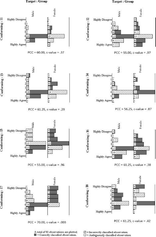
Multigrams, PCC indices, and c-values for eight Need for Speed items.
Finally, conducting independent samples t tests on the eight individual items also reveals the dilemma. Only Item 7 yields a statistically significant difference between men and women. Aggregating the eight items essentially buried the salient difference between the two sexes on Item 7 while creating the illusion that important, “statistically significant,” differences were assured on the other items as well since they measured the same quality.
This example and the anorexia study above demonstrate why a motto in Observation Oriented Modeling is “aggregation often leads to obfuscation.” To be clear, aggregation is meant to express the standard methods of computing means, variances, and covariances and all of the complex statistical methods based on these statistics. Aggregation may also refer to the simple tallying of responses or behaviors, a procedure common in the OOM software. The next generation must finally shed the “physics envy” and phenomenalism of modern psychologists who view the whole of science as continuous, quantitative measurement of qualities that are not truly knowable. Counting, or working with discrete quantities or units, underlies continuous measurement; hence, there is no shame or second class citizenship to be feared in dealing mainly with discrete quantities or speaking in terms of structures and processes rather than alleged continuous variables. It can also be noted that in Table 3, quantity is only one of Aristotle's ten categories of being.
With regard to Need for Speed, then, what alternatives might be pursued? Students can be encouraged to develop behavioral checklists, obtained via self-report or observation, as well as single-item approaches. Medical doctors often employ checklists to aid in diagnosis and treatment, and Barrett (2008) offers the Violence Risk Assessment Guide as a successful example checklist (accurately predicting violent recidivism at 72%) developed without the use of latent variable models or other sophisticated statistical models. With regard to single-item self-report approaches, they have been shown to be adequate replacements for multiple-item questionnaires in a number of contexts (e.g., see Nagy, 2002; Bergkvist & Rossiter, 2007). Rather than “measuring” extraversion with ten items, for instance, a single well-phrased item (Woods & Hampson, 2005) or a vignette can be developed:
An E-1 [extraverted] person is someone who tends to direct his or her energy toward the external world rather than to the inner world of ideas. Consequently, when presented with a new situation or unfamiliar activity, E-1s tend to jump right in without much hesitation. For instance, an E-1 attending a Yoga class for the first time with a friend would not hesitate to join in the exercises, or an E-1 visiting a sports bar for the first time would not feel uncomfortable in such a novel setting. E-1s, thus, tend to be seen as energetic and tend to seek out activities that involve other people. They also tend to be talkative, even in large groups of people, and they can sometimes appear to be aggressive when interacting with other people, even strangers (Brown & Grice, 2011, p. 3).
The person reading the vignette can be asked to affirm or deny the description as applying to himself or herself, thus avoiding a Likert-type or other form of rating scale. Using vignettes, in particular, requires students to think more deeply and concretely about the meanings of the qualities they are attempting to research. Behavioral checklists and single items will also yield units of observation more readily incorporated into integrated models because students will have to take greater responsibility in articulating the exact meaning of any numerical values they obtain.
From Statistical Replication to Model Building
It cannot be emphasized enough that any truly scientific progress in psychology will likely depend upon the development of integrated models. It has been argued above that variable-based models tested with modern statistics are superficial in most instances and downright misleading in other instances. These models, rooted in phenomalism (see Table 1), can also grow tediously complex. Some are introduced with ten or more variables linked together in a network of statistical associations (e.g., van Kampen, 2005) while others are built more gradually through a process known as replication-extension (Bonett, 2012). With regard to this latter process, for instance, recall the optimism/delay model for the breast cancer study above. After having established the statistically significant correlation in the original sample, a researcher may collect additional data for a new sample while adding another variable to the model,

The correlation between optimism scores and reported delay values is again tested for statistical significance, and if successful, the “effect” is said to have replicated. The optimism/delay correlations between the original studies can also be compared statistically, and if similar, combined into a single estimate of the posited population parameter. Students must be trained to understand correctly that “replication” here means something different than what they may have learned in their other science courses. In the context of null hypothesis significance testing, replication has an entirely statistical and probabilistic meaning. It simply means that the null hypothesis has been rejected in another sample, or that the statistics (e.g., correlations) from the two samples are not significantly different. Of course statistical power and the formal probabilities for Type I, Type II, and Type III errors (Harris, 1997) can all be discussed to help insure students' proper understanding of the statistical nature of these conclusions. Advanced students can additionally be asked to read the recent attempts to develop a p-replication statistic, which ultimately failed (Killeen, 2005; Maraun & Gabriel, 2010). Beyond these statistical concerns, replication-extension potentially represents a more troubling esoteric use of the word “replication” by psychologists. Imagine, for instance, if a different optimism questionnaire was used in the second, follow-up study. Can the tested association between the optimism scores and reported delays in the second study be called a replication of the first study? In more dramatic fashion, psychologists may change entire methodologies and still refer to subsequent studies as replications as long as two variables with the same labels can be statistically associated or as long as the “effect” being studied can be referred to in general terms, such as the “bystander effect” or “Barnum effect.”
At the root of this statistical and haphazard approach to replication is phenomenalism and a failure to recognize that causes inhere in the things themselves. A useful class exercise is to select a complex variable-based model from the literature and ask students to imagine tracing any given person through the network in a way that reflects a causal understanding of the structures and processes at work. Even attempting to determine what the actual values (scores) should be for a given person across all of the variables in the model can be challenging or impossible. Recent studies by Grice, et al. (2012) and Brown and Grice (2012) show how this type of empirical tracing of values through a model can be accomplished with the OOM software and how conclusions based on patterns of observations for individuals in the study can be markedly different from conclusions based on statistically significant associations between variables.
Variable-based models are simply not generally useful for explicating the causal structure of nature even if the statistical results from such models are “replicated” across studies. Consider Burger's (2005) recent attempt to duplicate much of the methodology in Stanley Milgram's famous 1963 study. Burger found that 70% (n = 28) of the participants in his study delivered shock after reaching the 150–volt level, which compared favorably to 82.5% (n = 33) observed by Milgram. Students can haggle over whether or not it is appropriate to judge the former percentage as replicating the second or to deem the difference as merely “inconclusive” (Bonett, 2012), but such efforts would miss the point by leading them right back into the world of statistics. What students really want to know is “why did each of the 28 persons deliver the apparently excessive shock, and why did each of the other 12 individuals decide not to administer the shock?” Burger acknowledges that psychologists don't have an answer to this scientific, causal question stating only that the studies “…are dramatic demonstrations of how individuals typically underestimate the power of situational forces when explaining another person's behavior” (2005, pp. 2–3). What is unfortunately not widely admitted or understood, however, is that population parameter-chasing schemes and variable-modeling strategies are not capable of answering such questions.
Different types of models are simply going to be required, and as a final example of integrated modeling, imagine speed measurements collected for a car traveling along a highway. The speed of the car along the level road is fairly steady (75 mph), fluctuating by less than ½ mph. The car then reaches a steep incline, and its speed quickly drops by 5 mph, but then gradually accelerates to, and holds relatively steady at 75 mph. The car then passes over the crest of a hill and accelerates momentarily by 4 mph before reducing its speed to 75 mph. What is the causal explanation for these observations? Why would an incline cause the car to first decelerate and then accelerate? Does the crest of a hill cause the car to first accelerate and then decelerate? No appeal to aggregate statistics or latent variables is necessary here, and a simple A → B → C efficient causal model is inadequate. With Aristotle's four causes under their belts, students should realize on their own that the car is adjusting its speed according to a final cause, the cruise control set to 75 mph. They should also realize that an integrated model is needed to explain the observations. In this case it would be a feedback loop model like the simple model of neuromuscular control introduced by Wiener (as cited by Powers, 1973) and shown in Fig. 13.

Feedback model of neuromuscular control system.
This simple diagram may generally be referred to as an efficient cause model, but Powers systematically builds upon this diagram to create a more complex model that can accommodate a final cause, like the cruise control setting in the car (Powers, 2008). Figure 14 shows Powers' model that can be used quite effectively for modeling tracking tasks; for instance, a person tracking a target across a computer screen or a person attempting to maintain the position of the screen cursor in the midst of various disturbances. Tracking tasks are obvious goal-directed behaviors, thus involving final cause. Moreover, Powers is clear that the testing ground for the accuracy of the model as a representation of a natural system is at the level of the persons doing the tracking, not at the level of aggregate statistics. Even in terms of replication, results should be repeatable for each and every person conducting the tracking tasks. This focus on the person, as well as the importance of goals, has led some psychologists to develop therapeutic techniques or models for clinical psychologists based on more elaborate variations of the model shown in Fig. 14 (see Mansell, 2005; Goldstein, 2007). The take-home message here is that Powers' approach to model building is radically different from the approach of most modern psychologists. His approach is truly causal, systematic, and scientific.

General model of feedback control system. Adapted from Powers (1973), p. 61.
Of course, understanding the parts, functions, and powers of an automobile or a person will not always involve employing feedback loops like those above. Other research efforts may be more like sleuthing for a particular thing or process operating as a cause, such as when a doctor attempts to diagnose a patient, e.g., pain in the bridge of the nose accompanied by headache, fever, and a sore throat may indicate sinusitis; whereas pain in the bridge of the nose accompanied by headache, fever, redness and swelling may indicate cellulitis. These symptoms can be expressed using symbols of logic as follows:
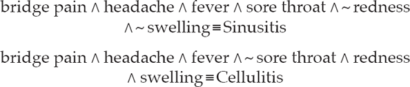
Searching for such patterns is referred to as logical hypothesis testing, and Grice (2011, pp. 203–205) reports an example contrived data set in which students can search for the formal cause of attempted suicides.
According to Doroughty, “A scientific explanation shows how the patterns discerned amid the flux of events are produced by the persisting natures and constitutions of things” (2013, p. 50). Observation Oriented Modeling, based on philosophical realism, is entirely consistent with this view. The OOM software has moreover been specifically designed to identify patterns within observations, and it provides a clear advantage over traditional statistical methods because of the transparency of the results (e.g., the graphical output, PCC indices, and c-values). By teaching students to think in terms of causes and effects rather than networks of variables, and to search for patterns rather than statistically significant associations in the aggregate, we may strike out into new frontiers, gaining a richer view of human persons and our place in the Order of Nature.
Footnotes
2
The OOM software can be downloaded for free at http://www.idiogrid.com/OOM. Additional information regarding the software and the Observation Oriented Modeling book (Grice, 2011). can also be found at this website.
3
All of data files in both SPSS and OOM formats can be found on the Observation Oriented Modeling website: ![]() . In addition, instructional videos can be found on the website for the examples discussed in this paper. These videos demonstrate how the analyses are conducted and interpreted using the OOM software.
. In addition, instructional videos can be found on the website for the examples discussed in this paper. These videos demonstrate how the analyses are conducted and interpreted using the OOM software.
Appendix
Need for Speed Contrived Data

| I1 | I2 | I3 | I4 | I5 | I6 | I7 | I8 | Group | Sum | |
|---|---|---|---|---|---|---|---|---|---|---|
| person_1 | 4 | 3 | 5 | 4 | 1 | 5 | 4 | 1 | 1 | 27 |
| person_2 | 5 | 5 | 0 | 4 | 3 | 5 | 4 | 3 | 1 | 29 |
| person_3 | 5 | 4 | 5 | 5 | 5 | 6 | 5 | 5 | 1 | 40 |
| person_4 | 4 | 4 | 4 | 5 | 2 | 4 | 5 | 2 | 1 | 30 |
| person_5 | 4 | 4 | 5 | 2 | 1 | 5 | 2 | 1 | 1 | 24 |
| person_6 | 4 | 6 | 4 | 4 | 4 | 4 | 4 | 4 | 1 | 34 |
| person_7 | 4 | 4 | 5 | 4 | 0 | 4 | 4 | 5 | 1 | 30 |
| person_8 | 4 | 4 | 0 | 3 | 3 | 6 | 3 | 2 | 1 | 25 |
| person_9 | 5 | 5 | 3 | 4 | 3 | 4 | 4 | 3 | 1 | 31 |
| person_10 | 4 | 3 | 4 | 4 | 4 | 2 | 4 | 4 | 1 | 29 |
| person_11 | 4 | 4 | 4 | 6 | 4 | 6 | 6 | 4 | 1 | 38 |
| person_12 | 3 | 5 | 4 | 4 | 5 | 6 | 4 | 5 | 1 | 36 |
| person_13 | 5 | 6 | 5 | 4 | 4 | 6 | 4 | 4 | 1 | 38 |
| person_14 | 3 | 3 | 4 | 3 | 0 | 2 | 6 | 0 | 1 | 21 |
| person_15 | 4 | 4 | 2 | 3 | 2 | 2 | 3 | 2 | 1 | 22 |
| person_16 | 5 | 2 | 3 | 4 | 0 | 0 | 4 | 0 | 1 | 18 |
| person_17 | 4 | 4 | 2 | 4 | 3 | 5 | 4 | 3 | 1 | 29 |
| person_18 | 4 | 6 | 5 | 5 | 4 | 4 | 5 | 4 | 1 | 37 |
| person_19 | 4 | 4 | 5 | 3 | 4 | 5 | 4 | 4 | 1 | 33 |
| person_20 | 2 | 2 | 0 | 4 | 3 | 5 | 3 | 3 | 1 | 22 |
| person_21 | 4 | 5 | 4 | 5 | 3 | 3 | 6 | 3 | 1 | 33 |
| person_22 | 4 | 3 | 5 | 4 | 1 | 4 | 1 | 1 | 1 | 23 |
| person_23 | 2 | 2 | 5 | 3 | 4 | 0 | 3 | 2 | 1 | 21 |
| person_24 | 5 | 5 | 6 | 6 | 5 | 1 | 5 | 4 | 1 | 37 |
| person_25 | 2 | 2 | 4 | 4 | 3 | 4 | 5 | 2 | 1 | 26 |
| person_26 | 5 | 5 | 4 | 4 | 3 | 4 | 2 | 3 | 1 | 30 |
| person_27 | 4 | 4 | 4 | 4 | 3 | 4 | 3 | 2 | 1 | 28 |
| person_28 | 5 | 5 | 5 | 4 | 4 | 5 | 4 | 5 | 1 | 37 |
| person_29 | 4 | 4 | 4 | 4 | 4 | 5 | 4 | 4 | 1 | 33 |
| person_30 | 4 | 3 | 5 | 5 | 5 | 5 | 4 | 5 | 1 | 36 |
| person_31 | 5 | 6 | 5 | 4 | 4 | 4 | 2 | 4 | 1 | 34 |
| person_32 | 4 | 4 | 4 | 2 | 2 | 4 | 2 | 2 | 1 | 24 |
| person_33 | 4 | 4 | 4 | 4 | 2 | 4 | 1 | 2 | 1 | 25 |
| person_34 | 5 | 4 | 1 | 5 | 4 | 6 | 4 | 4 | 1 | 33 |
| person_35 | 4 | 5 | 4 | 2 | 3 | 5 | 2 | 3 | 1 | 28 |
| person_36 | 4 | 4 | 4 | 4 | 4 | 4 | 4 | 4 | 1 | 32 |
| person_37 | 4 | 3 | 4 | 1 | 1 | 4 | 0 | 1 | 1 | 18 |
| person_38 | 4 | 1 | 4 | 4 | 3 | 4 | 5 | 4 | 1 | 29 |
| person_39 | 4 | 6 | 4 | 5 | 3 | 6 | 3 | 5 | 1 | 36 |
| person_40 | 1 | 1 | 1 | 1 | 0 | 2 | 1 | 0 | 1 | 7 |
| person_41 | 0 | 0 | 1 | 0 | 0 | 1 | 0 | 0 | 2 | 2 |
| person_42 | 3 | 3 | 1 | 1 | 1 | 2 | 0 | 1 | 2 | 12 |
| person_43 | 3 | 3 | 2 | 4 | 2 | 5 | 1 | 2 | 2 | 22 |
| person_44 | 6 | 6 | 5 | 4 | 0 | 4 | 0 | 0 | 2 | 25 |
| person_45 | 2 | 1 | 4 | 4 | 1 | 4 | 1 | 1 | 2 | 18 |
| person_46 | 4 | 5 | 5 | 4 | 4 | 4 | 4 | 4 | 2 | 34 |
| person_47 | 5 | 5 | 4 | 5 | 4 | 4 | 3 | 6 | 2 | 36 |
| person_48 | 4 | 4 | 5 | 6 | 5 | 6 | 4 | 4 | 2 | 38 |
| person_49 | 1 | 1 | 2 | 4 | 0 | 1 | 4 | 0 | 2 | 13 |
| person_50 | 4 | 4 | 4 | 4 | 2 | 1 | 0 | 2 | 2 | 21 |
| person_51 | 3 | 2 | 2 | 4 | 1 | 3 | 1 | 4 | 2 | 20 |
| person_52 | 4 | 6 | 4 | 5 | 4 | 4 | 3 | 4 | 2 | 34 |
| person_53 | 4 | 4 | 2 | 4 | 2 | 2 | 1 | 2 | 2 | 21 |
| person_54 | 2 | 2 | 3 | 1 | 3 | 2 | 0 | 3 | 2 | 16 |
| person_55 | 2 | 1 | 2 | 3 | 3 | 2 | 1 | 3 | 2 | 17 |
| person_56 | 6 | 6 | 6 | 4 | 5 | 6 | 4 | 4 | 2 | 41 |
| person_57 | 4 | 5 | 4 | 4 | 3 | 5 | 3 | 4 | 2 | 32 |
| person_58 | 3 | 2 | 0 | 1 | 0 | 2 | 0 | 0 | 2 | 8 |
| person_59 | 5 | 6 | 4 | 2 | 3 | 3 | 0 | 4 | 2 | 27 |
| person_60 | 4 | 4 | 2 | 4 | 3 | 3 | 2 | 1 | 2 | 23 |
| person_61 | 5 | 5 | 4 | 4 | 4 | 5 | 2 | 0 | 2 | 29 |
| person_62 | 2 | 3 | 4 | 1 | 2 | 2 | 2 | 1 | 2 | 17 |
| person_63 | 5 | 4 | 5 | 4 | 2 | 4 | 2 | 4 | 2 | 30 |
| person_64 | 5 | 5 | 4 | 3 | 3 | 3 | 3 | 2 | 2 | 28 |
| person_65 | 4 | 3 | 4 | 4 | 4 | 6 | 0 | 5 | 2 | 30 |
| person_66 | 4 | 5 | 4 | 4 | 3 | 3 | 2 | 2 | 2 | 27 |
| person_67 | 4 | 6 | 4 | 4 | 1 | 4 | 4 | 0 | 2 | 27 |
| person_68 | 2 | 0 | 2 | 5 | 0 | 4 | 1 | 4 | 2 | 18 |
| person_69 | 4 | 4 | 3 | 4 | 3 | 3 | 1 | 0 | 2 | 22 |
| person_70 | 4 | 4 | 4 | 3 | 3 | 4 | 2 | 0 | 2 | 24 |
| person_71 | 4 | 5 | 3 | 4 | 3 | 3 | 3 | 4 | 2 | 29 |
| person_72 | 4 | 4 | 4 | 3 | 3 | 4 | 3 | 5 | 2 | 30 |
| person_73 | 4 | 6 | 1 | 0 | 5 | 5 | 4 | 2 | 2 | 27 |
| person_74 | 5 | 4 | 5 | 3 | 4 | 5 | 3 | 4 | 2 | 33 |
| person_75 | 4 | 4 | 4 | 5 | 4 | 5 | 4 | 4 | 2 | 34 |
| person_76 | 6 | 2 | 5 | 5 | 4 | 6 | 4 | 4 | 2 | 36 |
| person_77 | 5 | 5 | 2 | 4 | 4 | 4 | 4 | 2 | 2 | 30 |
| person_78 | 4 | 4 | 5 | 4 | 3 | 5 | 3 | 4 | 2 | 32 |
| person_79 | 4 | 4 | 3 | 4 | 3 | 5 | 2 | 2 | 2 | 27 |
| person_80 | 4 | 4 | 4 | 3 | 2 | 5 | 2 | 4 | 2 | 28 |