
Abstract
Predicting the factor structure of a test and comparing this with the factor structure, empirically derived from the item scores, is a powerful test of the content validity of the test items, the theory justifying the prediction, and the test's construct validity. For the last two decades, the preferred method for such testing has often been confirmatory factor analysis (CFA). CFA expresses the degree of discrepancy between predicted and empirical factor structure in X2 and indices of “goodness of fit” (GOF), while primary factor loadings and modification indices provide some feedback on item level. However, the latter feedback is very limited, while X2 and the GOF indices appear to be problematic. This will be demonstrated by a selective review of the literature on CFA.
For construct validation of psychopathology and personality questionnaires, researchers often make use of confirmatory factor analysis (CFA), especially when the tests are supposed to be multidimensional. For this, a covariance matrix is calculated over the scores of a number of subjects and CFA is then applied to test whether a presumed factor structure or pattern is not contradicted by this matrix. CFA is executed by means of structural equation modeling (SEM), a very sophisticated statistical procedure for testing complex theoretical models on data. CFA is only used for the measurement part of the models. Since a computer program became available for SEM (LISREL; Jöreskog & Sörbom, 1974), this method has gained much in popularity. LISREL has been updated several times (Jöreskog & Sörbom, 1988), and there are several similar programs available now, e.g., Amos (Arbuckle, 2004; now included in SPSS), EQS (Bentler, 2000–2008), and Mplus (Muthén and Muthén, 1998–2010). All these can run on current personal computers, so the threshold to using CFA has become very low.
However, problems with the method have also increasingly been reported, especially since the turn of the century (e.g., Breivik & Olsson, 2001; Browne, MacCallum, Kim, Andersen, & Glaser, 2002; Tomarken & Waller, 2003). Current users of the method, working in the applied social sciences, may be less aware of these limitations of CFA than statisticians are and be over-optimistic about the reliability of the method when striving to validate questionnaires. The current paper is primarily meant for them. Researchers well initiated in statistics will probably find little new in it, but to see the problems recapitulated in a systematic way may motivate them to take note of the alternative approach to goodness-of-fit which I briefly sketch in the last section. Also, the two cautious explanations of puzzling findings, suggested in later sections, may invite them to dispute.
Test scales are devised to measure certain abilities or skills, whereas questionnaire scales are devised to measure, for instance, certain personality traits, diagnostic categories, or psychological conditions. So there is much difference between test items which provide an objective correct–incorrect score and questionnaire items which provide a subjective rating of oneself or another person, often on a quasi-interval scale of 3 to 10 points. Nevertheless, questionnaires are often referred to as tests in literature. For reasons of convenience the term “test” will be used interchangeably with “questionnaires” in this paper as well, yet it should never be interpreted as meaning a measure of aptitudes and abilities. This paper is about questionnaire validation only.
Item Clustering as Feedback on a Test's Theoretical Basis and Validity
Because they are meant to tap an aspect of a certain construct, the items within a questionnaire are supposed to have at least modest inter-correlations and should cluster. If a questionnaire is supposed to measure several distinct qualities, then the items should show a clustering corresponding to these various subscales.
It follows that an empirically found item clustering that corresponds to the ideas that guided the construction of the questionnaire is strong support for these ideas, as well as for the content validity of the items and the construct validity of the questionnaire. If the predicted clustering differs vastly from the empirically found clustering, the theory behind it could be considered faulty, and/or the test scale a mistaken operationalization, provided a good sample has been drawn. However, if the difference is moderate the discrepancies could be used to refine the theory and/or for further improvement of the measuring instrument.
The discrepancy could involve a low or opposite correlation of an item with its predicted scale. This may imply that the item is either poorly formulated or a poor operationalization of the phenomenon it represents, or that there is a flaw in the theory. The discrepancy could also involve a high correlation between an item and a scale to which it had not been assigned. In that case, the theory probably needs modification. Other flaws are: a correlation between two scales is much higher than expected, even to the point that the two scales could be considered as forming a single one-dimensional scale; or it is much lower than expected. In both cases, the theory will need to be reformulated to some extent.
Methods For Testing a Predicted Item Clustering
How does one test and evaluate the empirical clustering in relation to an a priori cluster prediction? A very direct and controlled way would be to examine the correlations between the items and the predicted scales (the latter are mostly operationalized as the unweighted sum of the item scores). These correlations should be in line with the prediction, and to the extent that they are not they offer a basis for revising the scales in the direction of greater homogeneity and independence. This method is known as item analysis (along the lines of classical test theory, not of item response theory!); many test developers make use of it. If the clusters are indeed revised, the revision must be performed iteratively in a very gradual manner (Stouthard, 2006), because after each modification the entire picture of clusteritem correlations will change. Test devisers do not go to extremes with these modifications because it is not wise to mold one's well thought-through test to every whim of imperfect empirical data.
Although this type of item analysis appears to be tailored for testing (and revising) cluster predictions, statisticians are uncomfortable about relying so totally on zero-order correlations between raw item scores and on equating cluster scores with the unweighted sum of the test scale items. Common factor analysis seems a better option because in this approach the variance per item is divided into a common part (common with the factor on which the item loads) and a unique part (item-specific variance plus error). Principal axis factor analysis is the most applied form of common factor analysis. It has partly replaced principal component analysis, which is based on the undivided variance of variables. In factor analysis all variables contribute—with a greater or smaller weight—to each factor.
However, these are examples of exploratory factor analysis (EFA). EFA is applied to data without an a priori model. It traces dimensions within a covariance or correlation matrix to the point at which enough variance has been explained. To further optimize these dimensions rotation is performed: orthogonal, when independent scales are expected, and oblique, when some of the dimensions are expected to correlate moderately or highly (up to a ceiling). The resulting factors may be compared to the presumed test scales: are the items of Scale A the ones loading highly on Factor X, those of Scale B on Factor Y, etc.? And are they loading much lower on a different factor? Is the correlation between the factors in line with the expected scale correlations?
The disadvantage of this often applied approach may be that the empirical factor structure/pattern 3 is too much affected by incidentally extreme item inter-correlations or by over- or under-representation of certain items, yielding factors that differ in number and content from the test scales. When a result is due to unrepresentative properties of the correlation/covariance matrix, such a result need not indicate a faulty prediction. However, adjusting the predicted structure/pattern to the data without unnecessarily giving up the prediction, on the one hand, and not violating the data on the other seems a less vulnerable procedure. CFA offers a way to achieve this, based on common factor analysis with its division in common and unique variance of the variables. How does this work?
Testing Predicted Factor Structure by Means of CFA
The prediction of the factor structure/pattern of a test involves the number of factors and the specification of the test items that define each factor (the so-called indicators), i.e., those which are expected to have high to moderately high loadings (or beta coefficients) on the factor. The investigator will most likely also have expectations about the correlation between the factors and perhaps about some cross loadings. Unique variance of the observed variables is also part of the model. These covariances, as well as the variances of the variables involved, are the parameters of the measurement model.
To test this predicted factor structure/pattern with CFA, the following procedure is applied:
The measurement model is translated “back” into a crude covariance matrix over all measured variables.
This covariance matrix is then adjusted to the empirically found sample covariance matrix in a number of iterations, mostly by means of maximum likelihood estimation (MLE). This is done in such a way that the difference between the two is minimized without violating the data too much. The final result is the implied covariance matrix.
For this process to come to an end and produce a result that helps to evaluate the model, the prediction must have been detailed enough, or, in SEM jargon, the model has to be over-identified. A model is over-identified when the number of known elements (non-redundant variances plus covariances of the sample matrix 4 ) exceeds the number of unknown parameters that have to be estimated by the iterative process.
Parameters that have to be estimated are: primary factor loadings of the indicators (mostly except one), factor variances and covariances (when not explicitly predicted to be very high or low), and error variances. The error covariances that are expected to correlate non-negligibly (an indicator inter-correlation beyond the result due to the common factor), if any, have to be added to this number; the others will not be estimated.
Parameters that are fixed at a certain value will not be estimated. Usually, one indicator per factor is fixed at 1 (non-standardized value) for the sake of adjusting the scaling of the factor to that of the indicators. Secondary factor loadings (non-indicators) are fixed at 0, except when a cross-loading is probable; then it has to be estimated. If the model prescribes an orthogonal factor structure, the factor covariances are fixed at 0; if the model prescribes a clearly oblique structure, they are fixed at 1; otherwise, they are to be estimated. Error covariances that are thought to be negligible have to be fixed at 0. (Fixing at 1 does not imply a correlation of 1.)
The fixed parameters strongly affect the adjustment procedure mentioned in point 2 by constraining it. The estimation of the non-fixed parameters is free, albeit steered by the model.
This procedure of iteratively adjusting the model matrix to the sample matrix replaces the orthogonal or oblique rotation of factors (maximizing high primary factor loadings and minimizing low cross-loadings), which is typical of EFA.
The resulting implied covariance matrix is compared with the sample covariance matrix. The difference is the residual covariance matrix. It may be standardized to facilitate interpretation.
This provides a basis for calculating the degree in which the predicted factor structure/pattern fits the data. If the residual covariances are, on average, small enough, then the model fits the data well.
These differences are expressed in χ2, with degrees of freedom (df) equaling the number of known parameters minus the number of unknown, non-fixed parameters, thus parameters that will be estimated. See Points 4 and 5 for more details.
This χ2 should be small enough—in relation to df—to be merely the result of chance deviations in the sample with respect to the population (when larger, it is ascribed to prediction errors).
The main source for the account above is Brown and Moore (2012; also see Brown, 2015).
Complications With χ2
The residuals, and thereby χ2, will often reflect an imperfection of the model, especially in the primary and intermediate phases of a research project. When this is the case, this feedback should be used for a revision of the theory and the SEM model. However, in the final stage of the research project, when the model has become well thought-out, the residuals will probably, on average, still deviate from zero. Now, the difference may merely or mainly be due to sample imperfections and fluctuations with respect to the population. Cudeck and Henly (1991) called the model imperfection error the approximation discrepancy, and the sample imperfection error the estimation discrepancy. When applying the χ2 test, the assumption is that, on the population level, the approximation discrepancy is zero (the prediction is perfect), so the empirically found difference on the sample level has to be only due to the estimation discrepancy (sample fluctuations). If the latter is small, then the null hypothesis, “the model does not hold for the population,” can be rejected.
How suited is the χ2 test for demonstrating statistical significance of a predicted factor structure/pattern by means of CFA? Conventionally, χ2 is used to express a difference between an empirically found distribution and the distribution to be expected based on a null hypothesis. This difference should be robust enough to hold—within the boundaries of the confidence interval—for the population as well. However, in CFA the difference should be the opposite of robust; i.e., the difference should be small enough to accept both the predicted factor structure/pattern and its generalization to the population. Therefore, paradoxically, χ2 should be statistically non-significant to indicate a statistically significant fit.
Demanding this may be asking for trouble. Indeed, with large samples (and SEM demands large samples), even very small differences may be deemed significant by current χ2 tables, suggesting a poor fit, in spite of the greater representativeness of a large sample. Many experts in multivariate analysis have thought this to be a problem. An exception to them is Hayduk. He argues that we should profit from χ2's sensitivity to model error and take the rejection of a model as an invitation for further investigation and improvement of the model (see Hayduk, Cummings, Boadu, Pazderka-Robinson, & Boulianne, 2007.) On SEMNET, 3 June 2005, Hayduk notes that “χ2 locates more problems when N is larger, so that some people blame chisquare (the messenger) rather than the culprit (probably the model).”
The other side of the coin is that models can never be perfect, as MacCallum (2003) contended, because they are simplifications of reality (see also Rasch, 1980, p. 92). Therefore, models unavoidably contain minor error. In line with this argument, there are always a few factors in exploratory factor analysis that still contribute to the total explained variance but so little that it makes no sense to take them into account. Thus, these factors should be ignored in CFA as well. Nevertheless, if the measurements are reliable and the sample is very large, such minor model error may yield a significant χ2 value, urging the rejection of a model that cannot further be improved.
What about expressing the approximation discrepancy? Is χ2 suited for that job? No, its absolute value is not interpretable: it must always be evaluated with respect to df and N. χ2 can only be used to determine the statistical significance of an empirically found value, the estimation discrepancy. Therefore, some statisticians also report χ2/df, because both χ2 and df increase as a function of the number of variables. This quotient is somewhat easier to interpret, but there is no consensus among SEM experts about which value represents what degree of fit.
Indices of Goodness of Fit
To cope with these complications and this problem, SEM experts have tried to devise other indices of “goodness of fit” or “approximate fit.” These should express the degree of approximation plus estimation discrepancy, and provide an additional basis for the acceptance or rejection of a model. All but one of these goodness-of-fit indices are based on χ2 and df, and some also include N in the formula. The remaining one (SRMR) is based directly on the residuals. Several suggestions have been made regarding their critical cutoff values (determining acceptance or rejection of a model), among which those of Hu and Bentler (1998, 1999) have been very influential.
Over the years, these indices have been investigated in numerous studies using empirical data and, more often, simulated data. Time and again they have been shown to be unsatisfactory in some respect; thus, adapted and new ones have been devised. Now, many of them are available. Only four of them will be mentioned below because they are often reported in CFA studies and they suffice to make my point. The formulas are derived from Kenny (2012), who, it should be noted, briefly makes several critical remarks in his discussion of the indices.
Standardized Root Mean Square Residual (SRMR; Jöreskog & Sörbom, 1988)
The most direct way of measuring discrepancy between model and data is averaging the residuals of the residual correlation matrix. This is what is done in SRMR: the residuals (Sij–Iij) are squared and then summed. This sum is divided by the number of residuals, q. (The residuals include the diagonal with communalities, so q=p (p + 1) / 2, where p is the number of variables.) Then, the square root of this mean is drawn. (In the formula below, S denotes sample correlation matrix, and I stands for implied correlation matrix.)

A value of 0 indicates perfect fit. Hu and Bentler (1998, 1999) suggest a cutoff value of ≤.08 for a good fit. Notice that x2 is not used to calculate SRMR.
Root Mean Square Error of Approximation (RMSEA, Steiger, 1990)
Root mean square error of approximation (RMSEA) has much more indirect relation with the residuals because it is based on χ2, df, and N. Its formula is

which could also be expressed as:

By dividing by df, RMSEA penalizes free parameters. It also rewards a large sample size because N is in the denominator. A value of 0 indicates perfect fit. Hu and Bentler (1998, 1999) suggested ≤.06 as a cutoff value for a good fit.
Tucker-Lewis Index (TLI; Tucker & Lewis, 1973)
The Tucker-Lewis Index, also known as non-normed fit index (NNFI), belongs to the class of comparative fit indices, which are all based on a comparison of the χ2 of the implied matrix with that of a null model (the most typical being that all observed variables are uncorrelated). Those indices that do not belong to this class, such as RMSEA and SRMR, are called absolute fit indices. Comparative fit indices have an even more indirect relation with the residuals than RMSEA. The formula of TLI is

Dividing by df penalizes free parameters to some degree. A value of 1 indicates perfect fit. TLI is called non-normed because it may assume values < 0 and >1. Hu and Bentler (1998, 1999) proposed ≤.95 as a cutoff value for a good fit. It is similar to the next index:
Comparative fit index (CFI; Bentler, 1990)
Here, subtracting df from χ2 provides some penalty for free parameters. The formula for CFI is
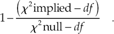
Values > 1 are truncated to 1, and values < 0 are raised to 0. Without this “normalization,” this fit index is the one devised by McDonald and Marsh (1990), the Relative Non-centrality Index (RNI). Hu and Bentler (1998, 1999) suggested CFI ≥.95 as a cutoff value for a good fit. Marsh, Hau, and Grayson (2005, p. 295) warned that CFI has a slight downward bias, due to the truncation of values greater than 1.0.
Kenny (2012) warned that CFI and TLI are artificially increased (suggesting better fit) when the correlations between the variables are generally high. The reason is that the customary null model (all variables are uncorrelated) has a large discrepancy with the empirical correlation matrix in the case of high correlations between the variables within the clusters, which will give rise to a much larger χ2 than the implied correlation matrix will. This affects the fractions in CFI and TLI, moving the quotient in the direction of 1. Rigdon (1996) was the first to raise this argument; later he advised using a different null model in which all variables have an equal correlation above zero (Rigdon, 1998).
Determination of Cutoff values by Simulation Studies
How do multivariate experts such as Hu and Bentler (1998, 1999) determine what values of goodness-of-fit indices represent the boundary between the acceptance and rejection of a model? They do so mainly on the basis of simulation studies. In such studies, the investigator generates data in agreement with a predefined factor structure/pattern, formulates correct and incorrect factor models, draws a great many samples of different sizes and observes what the values of a number of fit indices of interest will do.
One of the conveniences of simulation studies is that the correct and incorrect models are known beforehand, which provides a basis, independently of the fit index values, for determining whether a predicted model should be rejected or accepted. To express the suitability of the selected cutoff value of a goodness-of-fit index, the percentage of rejected samples is reproduced, i. e., the samples for which the fit index value is on the “rejection side” of the cutoff value. The rejection rate should be very small for correct models and very large for incorrect models. What percentage is to be demanded as a basis for recommending a certain cutoff value is often not stated explicitly by many researchers. It seems reasonable to demand a rate of ≤ 10% or even ≤ 5% for correct models and at least ≥ 90% or even ≥ 95% for incorrect models, considering that mere guessing would lead to a rate of 50% and p ≤.05 is conventionally applied in significance testing. A limitation of most simulation studies is that there are very few indicators (e.g., 3 to 6) per factor; usually, the number of items per scale of the typical tests or questionnaires is larger, especially in the initial stage of its development.
The study performed by Marsh, Hau, and Wen (2004), who replicated the studies of Hu and Bentler (1998, 1999), may serve as an example of this method for determining cutoff values.
Hu and Bentler had set up a population that corresponded to the following models: three correlated factors with five indicators each, with either (1) no cross-loadings, the simple model, or (2) three cross-loadings, the complex model. So the simple model had 33 parameters to estimate (3 × 4 factor loadings + 3 × 5 indicator variances + 3 factor covariances + 3 factor variances), whereas the complex model had 36 parameters to estimate (these 33, plus 3 additional factor loadings). With 15 variables, there were 15 × 16/2 = 120 known parameters. So the df for the true simple model was 120−33 = 87, and for the true complex model 120–36 = 84.
The misspecification in the simple model involved one or two factor correlations misspecified to be zero (orthogonal instead of oblique), whereas in the complex model one or two cross-loadings were overlooked (in other words: incorrectly held to be zero). So the df for the false simple models were 88 and 89, respectively, whereas those for the false complex models were 85 and 86, respectively.
The population of Marsh, et al. (2004) involved 500,000 cases. Samples of 150, 250, 500, 1,000, and 5,000 cases were drawn. (The number of samples was not mentioned.) MLE was applied. The dependent variable was the rejection rate per goodness-of-fit index with the cutoff value advised by Hu and Bentler (1999). Unlike Hu and Bentler (1999), Marsh, et al. (2004) calculated the population values of χ2 and the indices, which allows for a direct comparison of sample and population.
To provide the less initiated reader an idea of the results of such studies, a small portion of Tables 1a and 1b of Marsh, et al. (2004) is reproduced 5 in Table 1.
Cutoff Values and Related Percentage Rejection For RMSEA and SRMR (Marsh, et al. 2004)
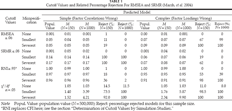
RNI replaces CFI here; see the section “Determination of Cutoff Values by Simulation Studies.”
Table 1 shows that the mean sample values of the first two fit indices are closer to the population values for N = 1,000 than those for N = 150. This result is observed because smaller samples have greater sample fluctuations.
It is further demonstrated that the population values (and mean sample values) of RMSEA for the simple model are below the advised cutoff values of Hu and Bentler (1999). In line with this observation, the rejection rate for N = 1,000 is 0%, whereas it should be ≥ 90%.
For the complex model, the population value (and mean sample values if N = 1,000) of SRMR is below the advised cutoff value; thus, the rejection rate is 0% whereas it should be ≥ 90%.
For RNI (comparable with CFI), the population values are on the acceptance side of the cutoff values in the two misspecified simple models and in the least misspecified complex model, and the rejection rates are accordingly.
Table 1 further shows that, ironically, χ2 performs better with respect to both models simultaneously than RMSEA and RNI, although it leads to more than 10% rejection of the correct models in three out of four cases.
This replication by Marsh, et al. (2004), therefore, did not confirm the advised cutoff values of Hu and Bentler (1999). Several of the misspecified models scored on the acceptance side of the cutoff values of the goodness-of-fit indices. Thus, what should be a cutoff value depends, first, on the type of misspecification one is interested in, and, secondly, on the degree of misspecification one is willing to tolerate for each type (Marsh, et al., 2004).
It can further be concluded from Table 1 that smaller samples may be problematic when assessing the correctness of a model: for N = 150, the mean RMSEA values for incorrect models are somewhat lower than the population values (decreasing the rejection rates), whereas the mean SRMR values for both correct and incorrect models are higher than the population values, increasing rejection rates for incorrect models (albeit insufficiently in this replication study). χ2, too, leads to an insufficient rejection rate for incorrect simple models in the case of the smallest misspecification.
SRMR seems to do very well in the case of the simple model (one or two factor correlations are zero instead of moderately positive), but Fan and Sivo (2005) showed that this was due to the fact that these zero factor correlations produce many zero variable correlations in the implied matrix, leading to large residuals and, consequently, a high SRMR because of its very direct relation to the residuals, more so than the other fit indices. If the factor correlations were misspecified to be 1 instead of merely high (meaning that the factors had to be fused), then SRMR no longer showed a special sensitivity to misspecified factor loadings.
Finally, note that only two kinds of misspecifications were investigated. Incorrectly assigned indicators and correlated error terms, for instance, were not modeled. This limits the degree to which the cutoff values may be generalized even more. Note further that even when the fit index values are beyond their cutoff criterion, they still hold some utility as measures of the approximation discrepancy.
Why Should One Draw Samples at All?
As indicated, Marsh, et al. (2004) calculated the population values of the fit indices, and when the values appeared to be rather far removed from an advised cutoff value, the rejection rates were close to 0% or 100%, depending on which side of the cutoff value each population value was. Chen, Curran, Bollen, Kirby, and Paxton (2008) reported similar experiences in their simulation study, which was designed to test the cutoff values for RSMEA (see the next section for more details regarding that study). In Table 2, the population values for the three correct and misspecified models are reproduced. Six out of nine population values for the misspecified models were below a cutoff value of 0.06 or even 0.05.
Population Values in the Study of Chen, et al. (2008, Derived From Their Table 1)

The information provided by the population values places one in a position to determine whether a selected cutoff value is too liberal, even before having drawn any sample. Thus, what is the use of drawing all those samples? Miles and Shevlin (2007) and Saris, Satorra, and van der Veld (2009) refrained from drawing any real sample and contented themselves with an imaginary sample of N=500 and N=400 respectively, perfectly “mirroring” the population values, saving themselves much calculation time [see Sections “Saris, Satorra, & van der Veld (2009)” and “Large Unique Variance Promotes an Illusory Good Fit” in the present article]. Sample drawing is only useful when the cutoff value is rather close to the population value because then the rejection rates, especially in the case of the smaller samples, are not obvious.
Reconciling Avoidance of Both Type I Error and Type II Error
In addition, cutoff values should be such that two types of error are avoided at the same time. They should be strict enough to avoid accepting a model when in fact it is incorrect, which represents a Type I error (a false positive). Alternatively, the cutoff value should be lenient enough to avoid rejecting a model that is correct, which represents a Type II error (a false negative). Can these two opposing interests always be reconciled, for any sample size, in CFA? Table 1 shows that the answer depends on the combination of model, sample size, and severity of misspecification for RMSEA, RNI, and SRMR. χ2 does not appear to be suited to reach 95% acceptance of correct models. In this case, the goodness-of-fit indices do better.
The study by Chen, et al. (2008), referred to in the previous section, offered an excellent opportunity for determining the degree to which both errors can be avoided at the same time, at any rate in the case of RMSEA. Chen, et al. (2008) investigated three models: (1) in Model 1, three factors with three indicators each plus one cross-loading indicator each; (2) in Model 2, three factors with five indicators each plus one cross-loading indicator each; and (3) like Model 1 but with four inter-correlating exogenous variables correlated with one factor and of which two variables also correlate with the other two factors. In Models 1 and 2, the misspecification involved omitting one, two, or three of the cross-loading indicators from the prediction. In Model 3, the smallest misspecification was omitting all three cross-loadings from the prediction, the moderate misspecification was omitting the four correlations of exogenous variables with the factors, and the largest misspecification combined the small and moderate misspecifications. The sample sizes were 50, 75, 100, 200, 400, 800, and 1000. The investigators generated 800 samples for each of the 84 experimental conditions.
The authors investigated the rejection rates for RMSEA cutoff points ranging from 0 to 0.15 with increments of 0.005. From their results it was clear that avoiding Type I and Type II error at the same time was often not possible for N ≤ 200. As an illustration of their findings, Table 3 shows what is inferred from their Figs. 4–15 for N=200 and N = 1000 only (this table is not a literal reproduction of one of their tables or a part of these, but is inferred from their Figs. 4–15). 6
Cutoff Values of RMSEA Required to Reach Good Rejection Rates (Chen, et al., 2008, Inferred From Figs. 4–15)

If N=200, only the moderate and severest misspecification in Model 3 allow for cutoff values that are suited for both accepting 90% or more correct models and rejecting 90% or more of incorrect models. In the seven other cases, no such cutoff values can be found. In three cases, even RMSEA = 0 is not strict enough to arrive at 90% rejection! For N = 1000, the results are much better: seven out of nine cases survived. However, the cutoff value that seems advisable based on this study would be 0.025 for N = 1000, which is most likely too strict for many other studies, especially for those with real data in which minor model error is unavoidable (MacCallum, 2003; see also Section “Three Degrees of Unique Variance and Their Effect on Goodness of Fit.” Moreover, a sample size of N = 1,000 is often out of reach in empirical studies with real data, especially in the field of psychopathology.
High Reliability (Small Unique Variance) Spoils the Fit
The variance in values for a variable within a set of variables is divided into common variance and unique variance. Common variance is a function of one or more features of the variables they have in common, and unique variance is a result of the influence of specific factors and measuring error. High common variance implies high correlations between the variables. If there is much error, i.e., low reliability, then the correlations between the linked variables are attenuated. In psychological research, making use of questionnaires or tests, there is often moderate reliability at best. However, in biological or physical research very reliable and homogeneous measurements are within reach. One would assume that this would be ideal for model testing.
Paradoxical Effect of a High Reliability
However, an article by Browne, et al. (2002) seemed to demonstrate the opposite. The researchers discussed data obtained from a clinical trial of the efficacy of a psychological intervention in reducing stress and improving health behaviors for women with breast cancer (Andersen, Farrar, Golden-Kreutz, Katz, MacCallum, Courtney, et al., 1998). One focus was on two types of biological responses of the immune system to the intervention. For each response there were four replicates. These 2 × 4 replicates were treated as indicators of two corresponding and related but distinct factors. Because the measures were biological and replicates, one may expect a high reliability and homogeneity among them, which implies a small unique variance. Indeed, on the face of it, the correlation matrix showed two distinct clusters of highly inter-correlating variables: 1–4 (M intercorrelation = .85) and 5–8 (M inter-correlation = .96). An MLE CFA was carried out hypothesizing these two factors. In spite of the clear picture (the residual matrix only contained values very close to zero) and the small sample (N = 72), x2 was significant, urging rejection of the model, and so did RMSEA and three other absolute GOF indices. The comparative fit indices RNI and NFI showed better performance but were nevertheless below the advised cutoff values. Only SRMR, with a value of 0.02, indicated acceptance of the model unambiguously, in line with the fact that this index is based on the residuals alone.
The researchers went on to frame a correlation matrix, consisting again of two clusters, but with much lower inter-correlations between the variables. Within the first “cluster” in particular the mean variable intercorrelation (its cohesion) was only .14, and the cohesion of the second cluster was .61, which is quite high but much lower than that of the original cluster. MLE CFA with a model for two related factors should yield the same residual matrix as above, and therefore the same SRMR, as indeed it did. The result: χ2 was no longer significant, thus indicating a good fit, in spite of the first cluster's unconvincing cohesion. The same held for the goodness-of-fit indices.
Browne, et al. (2002) concluded that χ2 and the fit indices based upon it measure detectability of misfit rather than misfit directly. In other words, the high statistical power of a test may easily lead to the rejection of a model, whereas a mediocre statistical power leads to the acceptance of the model (see also Steiger, 2000). In social science research, one is rarely confronted with this undesirable phenomenon because most measures are of moderate quality. Nevertheless, they may vary from rather reliable and homogeneous to mediocre. It would be ironic if only the latter would show good fit index values. Browne, et al. (2002) reasoned that this discrepancy is caused by the fact that, due to the procedure in CFA, χ2 is affected not only by the residual matrix but also by the sample matrix. Thus, it can be influenced by the degree of unique variance in the observed variables. Because all GOF indices but SRMR are based on χ2, they will indicate a poor fit as well.
Hayduk, Pazderka-Robinson, Cummings, Levers, and Beres (2005) against Browne, et al. (2002)
The data gathered in the study by Browne, et al. (2002) enjoyed a remarkable reanalysis by Hayduk, et al. (2005). These investigators had reason to believe that the two-factor model of Browne, et al. had not been correct and that two “progressively interfering” factors should have been included, which were thought to affect the respective two clusters of measurements. This alternative model appeared to fit the data very well, such that χ2 was far from significant in spite of the minute unique variance. Eliminating one of the progressively interfering factors from the model spoiled the results. The same held for a few other variations of the model.
From the section, “A Spurious Influence of the Number of Factors and Variables,” we can learn that a greater number of factors in proportion to the number of observed variables promotes the acceptance of incorrect models. So improving fit by introducing two additional factors into the model does, in itself, not prove the superiority of the χ2 test. The added factors should first make sense theoretically. I am not the one to judge that in the present case.
Mulaik (2010) proposed a further refinement of the model, which involved a correlation of .40 between each of the progressively interfering factors and the clusters of measures they were supposed to affect. This refinement did not improve the already good fit but was theoretically more plausible.
Saris, Satorra, and van der Veld (2009)
Saris, et al. (2009) reported a similar study: they devised population data for a one-factor model. Strictly speaking, the data were more precisely described by a two-factor model in which the correlation between the two factors was .95. This difference they considered trivial, so the one-factor model should have been deemed acceptable. The authors drew an imaginary, perfectly representative sample (N=400) from this population and calculated χ2, RMSEA, CFI, and SRMR. If the factor loadings were .85 or .90—which presupposes high reliability and low specific variance—then the values of χ2 and RMSEA led to the rejection of the one-factor model. Only CFI (in line with the expectations of Miles & Shevlin, 2007; see Section “Large Unique Variance Promotes an Illusory Good Fit”) and SRMR (not being χ2 based) had values in favor of acceptance of the model. If the loadings were decreased to ≤ .80, then χ2 and RMSEA also indicated acceptability of the two-factor model.
Conclusion
The lesson to be learned from the foregoing is that one should not be too eager to resist indications of ill fit simply because the unique variance is particularly small. A serious search for an alternative model should always be undertaken (Hayduk, Cummings, Pazderka-Robinson, & Boulianne, 2007; McIntosh, 2007). That does not mean, however, that indications of ill fit should never be considered trivial. However, the latter cannot automatically be concluded from a very small unique variance; it must be supported by substantive arguments.
Large Unique Variance Promotes an Illusory Good Fit
A much more important lesson to be learned from Browne, et al. (2002), however, is that non-significant χ2 and favorable goodness-of-fit index values cannot be trusted uncritically because these may merely be promoted by low intervariable correlations as a result of a large unique variance. Their findings do not stand alone. Some simulation studies have detected similar problems.
Miles and Shevlin (2007) reasoned that comparative fit indices might be more robust against the paradoxical influence of reliability because the former depend on the comparison of two χ2 values that should be approximately equally affected by the degree of unique variance in the observed variables. To test this, they devised a study in which they compared χ2, RMSEA, SRMR, and a number of comparative fit indices.
The authors set up a population, corresponding to two related factors (correlation 0.3) with four high-loading indicators each and two minor factors, the one loading very low on two indicators of the one major factor and the other loading very low on two indicators of the other major factor. Miles and Shevlin (2007) “drew” an imaginary sample of N=500, perfectly mirroring the population values. The tested model was a two-factor structure omitting the two minor factors. With a perfect reliability of 1.0, the disturbance by the minor factors was enough to have the model rejected by χ2. RMSEA indicated a doubtful fit, but the other fit indices indicated a good fit, as they were predicted to do. However, decreasing the reliability to a modest 0.8 resulted in χ2 and RMSEA both indicating a good fit, whereas the comparative indices and SRMR continued to indicate a good fit.
Miles and Shevlin (2007) performed a second study using this model, but left out the two minor factors while the correlation between the two factors was increased to 0.5. This time, the model tested was severely misspecified, a one-factor model. If the reliability was 0. 8, χ2 indicated misfit, as it should, and so did all of the fit indices. However, when the reliability was decreased to a meager 0.5, χ2 suddenly indicated a good fit and so did RMSEA and—in spite of not being χ2 based—SRMR. It was hoped that the comparative fit indices would be robust against the spurious influence of reliability on χ2, but only two of them were—the normed fit index (NFI; Bentler & Bonett, 1980) and relative fit index (RFI; Bollen, 1986). Three of them did not indicate misfit: CFI, TLI, and incremental fit index (IFI; Bollen, 1989).
Three Degrees of Unique Variance and Their Effect on Goodness of Fit
Stuive (2007; see also Stuive, Kiers, Timmermans, & ten Berge, 2008) investigated unique variance systematically as an independent variable.
Stuive's study was performed with continuous data, simulating a 12-item questionnaire with three subtests of four items each. The misspecification here was an incorrect assignment of one or more items to subtests (three levels; note that this is a much more serious prediction error than misspecified cross-loadings). In addition, 10% “minor model error” was introduced in one-third of the data and 20% in another one-third of the data, following the argument of MacCallum (2003) that 0% model error can never be realized in studies with real data. This “minor model error” consisted of the effect of nine unmodeled factors.
The independent variables were: (1) unique variance (25, 49, or 81%), (2) amount of minor model error, and (3) correlations between the three factors (.0, .3, or .7). Variables 1 and 3 were parameters to be estimated, not fixed; Variable 2 was not part of the model. The sample size was another independent variable: 50, 100, 200, 400, and 1,000 cases. For each combination of conditions, 50 samples were drawn.
The dependent variables were: the percentage of (a) accepted correct assignments and (b) rejected incorrect assignments. Acceptance of the assignments depended on the p value (> .05) of MLE χ2, as well as on different cutoff values for three fit indices and combinations thereof.
Figure 5.2 in Stuive (2007) shows that introducing 10% model error had a very strong effect on χ2 (p > .05), resulting in a decrease in the acceptance rate of correct models from approximately 92% to approximately 58%, over all unique variance conditions. Introducing 20% model error resulted in an acceptance rate of only 40%. If one finds 10% and 20% model error too large to be considered “minor,” then these results are in favor of using χ2 (p > .05), not against it. In spite of these strong effects, Stuive and her team joined together the cases with 0, 10, and 20% model error in order to study what the three degrees of unique variance did to the statistical power of CFA.
Rejection of Correct Models (Type II Error)
The samples N=50 and N = 100 will be ignored in this section and Section “Acceptation of Incorrect Models (Type I Error)” because they caused too much erroneous judgments in the cases of moderate and high unique variance. What was the effect of the degree of unique variance on the rejection of correct models (Fig. 5.1 in Stuive, et al., 2008)?
If the unique variance was 25%, approximately 70% of the correct models were rejected 7 based on χ2, p > .05. Of the fit indices, RMSEA and CFI needed their most lenient cutoff values (0.10 and 0.94, respectively) to reduce the rejection of correct models to approximately 10%. SRMR did not seem affected by a small unique variance: 0% of the correct models was rejected for N ≥ 200, even with the strict SRMR ≤ .06.
In the case of 49% unique variance, the rejection rate of correct models based on χ2 dropped only slightly below 70% for N = 1,000. For N=400 it decreased to approximately 50%, a score not above chance level. RMSEA and CFI, on the contrary, demanded little or no rejection of correct models, provided N ≥ 400. SRMR did well for N ≥ 200.
In the case of 81% unique variance, the rejection of correct models, based on χ2, dropped dramatically to approximately 15% for N = 1000 and 10% for N=400 (Stuive, 2007, Fig. 5.1c). In other words, the minor model error in the correct models no longer mattered much. The three goodness-of-fit indices scored well.
In all, a higher unique variance promoted the acceptance of correct models (decreasing Type II error). But did it also promote the acceptance of incorrect models (increasing Type I error)?
Acceptation of Incorrect Models (Type I Error)
The results are inferred from Stuive (2007, Fig. 5.4) and Stuive, et al. (2008, Fig. 2).
With 25% unique variance, the rejection rate was approximately 100%—justly so—for χ2, RMSEA, SRMR, and CFI, even with the most lenient cutoff values.
With 49% unique variance, the cutoff value for RMSEA had to be somewhat stricter (reject the model if RMSEA > .08) to reach approximately 90% rejection with N=400 and N = 1000. The same held for SRMR (reject the model if SRMR > .08). CFI and χ2 were still performing perfectly.
However, with 81% unique variance only the strictest cutoff value of RMSEA (reject the model if RMSEA > .03) led to an acceptable rejection rated (95% for N = 1,000 and 85% for N=400). Remember, using this strict value led to the rejection of “correct” models as well, in the case of unique variances of 25 and 49%. SRMR performed even worse: even the strictest cutoff value (reject the model if SRMR > .06) led to acceptance of (almost) all incorrect models, except for the small sample sizes (sic). CFI, on the contrary, continued to show good rejection rates, at least for N = 400 and especially N = 1000; this is in line with its greater robustness against a high unique variance, as assumed by Miles and Shevlin (2007). As to x2, for N = 1,000 it accomplished 100% rejection, as it should have; for N=400 it yielded 85% rejection, while for N ≤ 200 it rejected only 50% and less of the incorrect models.
To summarize: in line with the findings and reasoning reviewed in sections “High Reliability (Small Unique Variance) Spoils the Fit” and “Large Unique Variance Promotes an Illusory Good Fit,” MLE χ2 (p > .05), in case of small unique variance, demanded too much rejection of correct models (only if the data contained minor model error), whereas in case of large unique variance it allowed too much acceptance of incorrect models. Being χ2-based in a very direct manner, the same held for RMSEA, albeit to a much more attenuated degree. CFI was rather robust against the undesirable influence of unique variance. SRMR, however, appeared to lose its power to detect incorrect models as a consequence of high unique variance (81%, not 49%), in spite of not being χ2-based, even more so than RMSEA. This also put into perspective the favorable acceptance rates of SRMR regarding correct models, mentioned in the study of Browne, et al. (2002).
Large Unique Variance Combined With High Factor Correlation Promotes Type I Error
The results of Stuive (2007) with respect to incorrect models were reasonable when the unique variance was 49%, especially for CFI. However, this only held when the factors correlated 0.3 or 0.0, but not when the factors correlated 0.7. Then, a large unique variance caused the fit indices, including CFI, to lose their power to reject incorrect models altogether (see Fig. 5.5 in Stuive, 2007). Let us have a more detailed look.
With 25% unique variance, χ2 and RMSEA continued to reject incorrect models perfectly. SRMR rejected incorrect models perfectly only with the strictest cutoff value (reject model if ≤ .06), but was below the chance level with more lenient cutoff values. CFI, too, required the strictest cutoff value (reject model if CFI ≥ .96) to reject enough cases (approximately 90% with N=400 and N = 1000).
With 49% unique variance, only χ2 for N ≥ 200 led to (almost) perfect rejection of incorrect models. RMSEA then required the stricter cutoff value of 0.06, in combination with N ≥ 400, to reach 95–100% rejection (when the factor correlations were 0.0 or 0.3 the cutoff value 0.8 sufficed). The rejection rate for SRMR and CFI, however, was below chance.
With 81% unique variance, χ2 with N = 1000 sank to 85%, but below chance level for smaller sample sizes. RMSEA, SRMR, and CFI were no longer suited to reject incorrect models (almost 0% for the larger sample sizes). Remember, on top of the incorrect item assignments there was the minor model error in 67% of the models, which affected χ2 and RMSEA considerably if the factor correlation was still ≤.3.
In sum, from Stuive's (2007) simulation study (Sections “Three Degrees of Unique Variance and Their Effect on Goodness of Fit” and “Large Unique Variance Combined With High Factor Correlation Promotes Type I Error”) and from the studies discussed in Section “Large Unique Variance Promotes an Illusory Good Fit,” it can be concluded that the more “messy” the empirical factor structure/pattern is, the better the fit is suggested by SRMR and CFI and to a lesser degree by χ2 and RMSEA, even for the rather severely misspecified models that were typical for her study. Goodness of fit is increasingly over-estimated with higher unique variance, especially in combination with an unmodeled high factor correlation, thereby promoting Type I error (false positives).
The utmost consequence of this undesirable relation between unique variance and goodness of fit was drawn by Marsh, Hau, and Wen (2004), repeated in Marsh, et al. (2005, p. 318), where the authors stated, “… assume a population-generating model in which all measured variables were nearly uncorrelated. Almost any hypothesized model would be able to fit these data because most of the variance is in the measured variable uniqueness terms, and there is almost no co-variation to explain. In a nonsensical sense, a priori models positing one, two, three, or more factors would all be able to ‘explain the data’ (as, indeed, would a ‘null’ model with no factors). The problem with… this apparently good fit would be obvious in an inspection of… all factor loadings [which, then, all turned out to be] close to zero.”
Explanatory Suggestion
An explanation of the model-accepting effect of a “messy” factor structure/pattern is beyond the scope of this paper. However, I wonder whether the problems might be due to the element of comparing two complete correlation matrices. (a) If all correlations are relatively small (large unique variance), then the residuals will also tend to be small. This will artificially decrease SRMR and to a lesser degree χ2 and RMSEA, obscuring real misfit. (b) If the correlations between the indicators per factor are high, then their residuals will also tend to be high, obscuring real fit. For CFI and TLI, however, the opposite may hold because of a larger distance of the tested model to the null model (see the argument of Kenny, 2012, and Rigdon, 1996, mentioned in Section 5, last paragraph.) (c) For item clusters to hold, if the clusters are almost independent then the items within each cluster correlate much more highly with each other than with the items from the other clusters. On the other hand, if the clusters correlate highly, then the correlations of the items within a cluster will not be much higher than those of the items between clusters. Consequently, the residuals of incorrectly assigned items would be smaller in the case of highly correlating factors than in the case of independent factors. That would explain why a high factor correlation spoils the detection of misspecified models, as reported in this section (and promotes the acceptance of correct models: the other side of the coin!). For the reproduced correlation matrices in factor analysis of oblique structures/patterns this may hold to an attenuated degree, but the effect will not completely be flattened out.
A Spurious Influence of the Number of Factors and Variables
Breivik and Olsson (2001) reasoned and observed that RMSEA tends to favor models that include more variables and constructs over models that are simpler, due to the parsimony adjustment built in (dividing by df). These findings are in line with those of Meade (2008). Meade investigated the suitability of various fit indices to detect an unmodeled factor present in the data. This author observed that RMSEA ≤.06 was strict enough to detect the unmodeled factor, only if the factors consisted of four items. However, if the factors consisted of eight items each, ≤.06 appeared too liberal; in other words, the calculated RMSEA had become smaller than 0.06 (Fig. 9 in his article).
The same problem seems to hold for SRMR (Anderson & Gerbing, 1984; Breivik & Olsson, 2001; Kenny & McCoach, 2003). Fan and Sivo (2007) observed that SRMR performed much better for smaller models; in the larger models, the value of SRMR (not reproduced by the authors) was too small to reject misspecified models (their Table 3 vs their Table 2).
Explanatory Suggestion
Why do more factors relative to the number of variables result in a smaller SRMR? A full explanation is beyond the scope of this paper, but again a cautious suggestion can be made. For my argument, have a look at the Appendix. Four correlation matrices of 12 variables each are printed. Each matrix is ordered in such a way that the clusters of correlations, corresponding to the factors, can easily be detected. If there are two clusters with six indicators each, there are 42 within-clusters inter-item correlations (communalities included) against 36 between-clusters inter-item correlations. If there are three clusters of four items each, as in Stuive's (2007) study, then there are 30 within-cluster inter-item correlations against 48 between-clusters inter-item correlations. If there are four clusters of three variables each, then there are 24 within-clusters inter-item correlations against 54 between-clusters inter-item correlations. Finally, if there are six clusters of two items each, then there are 18 within-cluster inter-item correlations against 60 between-cluster inter-item correlations.
So, the more item clusters in relation to the total number of variables (except in the case of two clusters), the more the between-clusters inter-item correlations outnumber the within-factors inter-item correlations. In the case of an equal number of variables per cluster, this follows the formula:

in which w = the number of within-clusters residuals; b = the number of between-clusters residuals; v = the number of variables; and f= the number of variable clusters (factors).
Unless the factors are severely misspecified, the absolute values of the correlations that are not part of the factors will generally be much lower than those of the within-factors correlations, even if the factors intercorrelate moderately high, by definition so. This will hold for both the empirical and the implied matrix.
The difference between variable pairs with low correlations will mostly be smaller than the difference between variable pairs with high correlations. So the residuals of the between-factors inter-item correlations will generally be smaller than the residuals of the with-in-factors inter-item correlations (unless the factor correlations have been fixed to be 0 (see Fan & Sivo, 2005; also discussed in the section “Determination of Cutoff Values by Simulation Studies”).
In the case of many factors with few indicators each, these small between-factor inter-item residuals will outnumber the somewhat higher within-factor residuals. The average of all residuals together will then be smaller too. And this will result in a smaller value for SRMR, and—with some attenuation—a smaller RMSEA and χ2 as well. This suggests a better fit, even if the model is more or less misspecified.
CFA and Its Limited Feedback on Test Item Level
A limitation of CFA of an altogether different kind has to do with the feedback on the level of individual items. CFA is meant for a test of the measuring instrument as a whole: if χ2 and/or the goodness-of-fit indices assume unfavorable values, then the prediction could be considered refuted. However, such an all-or-nothing decision is not the only or main thing in which the researcher is interested, especially not in the early and intermediate phases of his investigation. Then the preference is for more detailed feedback, which enables him to improve the theory or test, or both (Anderson & Gerbing, 1988). Such feedback would be provided by a factor structure/pattern with factors, corresponding in number and nature to the predicted factor structure, yet completely in accordance with the empirical correlation matrix. The output of CFA, however, contains a factor structure/pattern that is strongly affected by the theoretical model behind the test, quite different from the structure/pattern resulting from exploratory factor analysis with oblique rotation: secondary factor loadings (beta-weights) are lacking because they were fixed at zero in the prediction, except where cross-loadings had been predicted (which, necessarily, concerns only a few indicators). So the researcher can see which items have a suspiciously low primary loading (standardized beta-coefficient), but not whether they should have been reallocated to another factor (and, if so, which one), or that they should be considered cross-loading.
The output also includes modification indices per parameter. These indices show to what extent χ2—and/or one or more of the goodness-of-fit indices—could adopt a better value (because of smaller residuals) by reallocating these items to another factor, or by assuming cross-loadings or different factor correlations. The researcher could “free” the fixed parameters with the poorest values and have them estimated by the iterative procedure used before or fix the free parameters with the poorest values. However, after such a modification, the whole picture of modification indices (and primary factor loadings of the items) will change, so the picture of modification indices in the initial stages cannot be relied upon to give accurate information on all items (parameters) simultaneously.
A further disadvantage is that CFA requires rather large samples to be reliable, especially in the case of a large number of variables; 5–10 observations per variable is often the advice. For the latter reason, scores of subtests or of item “parcels” are often preferred above single items to obtain reliable results. The items individually, however, are the very thing the cluster predictor or test deviser is interested in, and whether these can be combined into parcels has yet to be proven. 8 In addition, especially in the field of psychopathology, large samples are rarely realizable. Most of the time one has to content oneself with “convenience samples” of moderate size, i.e., samples selected non-randomly from a “poorly-defined super-population” (Berk & Freedman, 2003).
Factor analysis was invented to deal with a great number of correlating variables, producing massive covariance matrices. SEM was invented to test structural models with a limited number of theoretical constructs and a few observed variables, which, together, produce modest empirical and implied covariance matrices and whose residual matrices can be overviewed easily. For structural models, it makes sense to have a few measures that summarizes the fit of both matrices. For tests with a great number of items, this makes much less sense. Perhaps it was not a good idea in the first place to use SEM for confirmatory factor analysis as well.
Discussion
Even if it would also makes sense to have indices of goodness of fit in cases of a great number of observed variables, those that are produced by SEM are plagued by various problems:
χ2 may indicate misfit, especially in tests of high statistical power, simply because the sample is large. On the other hand, SEM requires large samples to do its job properly.
The goodness-of-fit indices do require large samples to discern good from poor predictions, in line with what SEM needs, but large samples are often out of reach in many psychological studies, especially in the field of clinical psychology.
When the reliability of a test is high and the specific variance of the variables is small (betraying itself in high correlations between the variables within a cluster), χ2 and RMSEA lead to the rejection of well-predicted models if there is minor model error. Minor model error, however, is unavoidable under real-world conditions. CFI is somewhat more robust against this effect.
On the other hand, when the reliability of a test is low, χ2 and RMSEA lead to the acceptance of poorly predicted models (comparative fit indices somewhat less).
When the unique variance of test variables is high (high specific variance and/or low reliability), then χ2 does not detect incorrect models when N ≤ 200. RMSEA does not detect misfit under any N. SRMR can no longer discern good fit from misfit. CFI requires a strict cutoff value and N ≥ 400.
When the factors have a high correlation (.70), while the unique variance is 49%, SRMR and CFI are no longer suited to reject incorrect models. If the unique variance rises to 81%, none of the fit indices is suited to reject incorrect models, except χ2 with an N = 1000.
There are also indications that increasing the number of factors relative to the number of variables spoil the power of RMSEA and SRMR to detect incorrect models.
So, on the basis of this selective review, reinforced by the brief theoretical suggestions in the sections “Large Unique Variance Combined with High Factor Correlation Promotes Type I Error” and “A Spurious Influence of the Number of Factors and Variables,” it must be concluded that, for a significance test of a model, χ2 and the GOF indices are too unreliable, and for an estimation of the approximation discrepancy, the GOF indices are too inaccurate. As early as 2007, such problems made Barrett call for their abandonment: “I would recommend banning all such indices from ever appearing in any paper as indicative of ‘model acceptability’ or ‘degree of misfit.’” (Barrett, 2007, p. 821). In addition, for feedback on the level of individual items CFA is not ideal.
Limitations
Part of the findings by Stuive and associates has to be put into perspective. It was interesting to see what happened to χ2 and the fit indices in the case of 81% unique variance, but such a high unique variance in a 3 × 4 item test implies a Cronbach's a of .50, as Stuive, Kiers, and Timmermans (2009) admit. Such tests will probably not be used in practice. The other extreme, a questionnaire with a unique variance of only 25%, will probably also be rare in psychology research; around 50% is more likely. But it is then that CFA yields its most practical results. So the skeptical conclusions above should not be taken to imply that all studies that have applied CFA are of questionable value. However, a critical attitude to such studies is certainly warranted.
Another limitation is that some of the criticisms may pertain more to the way CFA is applied by many researchers than to CFA as such, in the first place, leaving too many parameters free to estimate (for then, a good fit will be readily attained but does not say very much), or fixing too many (e.g., not including cross-correlations or correlated error terms in the model). A more complete and precise measurement model prediction will probably yield more reliable and meaningful χ2 and goodness-of-fit index values.
The criticisms raised in this article hold especially for CFA of tests with many items, not for SEM of structural models with only a few—both valid and reliable—indicators per factor in the measurement part. Besides, the objection of limited feedback at the item level becomes less relevant in an advanced stage of a research project when the test has gained good psychometric properties. Then, a global evaluation of approximate fit (GOF) and estimation fit (statistical significance) might be all the researcher needs.
Future Directions
What could be an alternative to, or an improvement of, CFA in the case of testing instruments with many variables when one is still in the early and intermediate stages of a research project?
Exploratory Structural Equation Modeling
In 2009, Asparouhov and Muthén introduced a variant of CFA that was called exploratory structural equation modeling (ESEM). This approach was intended to overcome the earlier mentioned limitations of CFA. In this method, in addition to a CFA measurement model, an EFA measurement model with rotations can be used within a structural equation model. There is no longer a need to fix the non-indicators per factor on 0. They can be freely estimated, and they are reproduced in the output. So there are secondary factor loadings.
The superiority of ESEM to CFA in cases of more complex measurement models has already been demonstrated in studies like Marsh, Ludtke, Muthèn, Asparouhov, Morin, Trautwein, et al. (2010), Furnham, Guenole, Levine, & Chamorro-Premuzic (2013), Booth and Hughes (2014), and Guay, Morin, Litalien, and Vallerand (2014). Also, ESEM could further be used for a data-driven model-modification with more realistic and informative results than CFA.
Data-driven Optimization of Predicted Clusters: A Fruitful Approach to Goodness of Fit
What would be the advantage of such “a data-driven model-modification”? That would result in factors that are congruent with the predicted ones on the one hand, but that are in good agreement with the empirical correlation or covariance matrix on the other: predicted indicators that appeared to have a insufficient factor loading would no longer be considered an indicator, while variables that have an unexpected high loading on a factor will now count as indicators. These modifications often imply that the clusters formed by the redistributed factor indicators have a better cohesion (average inter-variable correlation) than the corresponding predicted ones at the start.
Such a result would be comparable to that of item analysis, as explained in the section “Methods for Testing a Predicted Item Clustering,” but this time continued to the point at which the clustering neatly fits the empirical correlation matrix. If performed with ESEM, the result will be based on common factor analysis, which may be preferred by statisticians. Model re-specification with CFA based on the modification indices is also a possibility (Stuive, et al., 2009), but ESEM will probably lead to better results.
Whatever the method applied, such final factor structure/pattern (or cluster structure, as the case may be) will be extremely capitalized on chance and other sources of error, as MacCallum, Roznowski, and Necowitz (1992) warned. However, that would only be a problem if the revised factor structure would be adopted unconditionally as the better one, but that is not what it should be used for. Having a predicted factor structure on the one hand and an optimized factor structure on the other, the latter being continuous with the predicted one but in good agreement with the empirical correlation matrix at the same time, puts the researcher in a position for a detailed comparison of the two structures. And this generates detailed feedback on item level as well as a basis for a new kind of goodness-of-fit index. This will be explained briefly.
Indicators that are shared by both the predicted and its corresponding optimized factor can be considered correct positives; in other words, hits (H items). Indicators that had to be removed from the predicted factor to arrive at its corresponding optimized version can be considered false positives (F items). Indicators that had been missed in the prediction of the factor, corresponding with its optimized version, can be considered false negatives (M items). The number of H items, F items, and M items can now be combined in a simple formula:

Here, AP (it) stands for accuracy of prediction in terms of number of items, H for number of hits, F for number of F items, M for number of M items, Cp for size of the predicted cluster, and Cf for size of the final (optimized) cluster. A correction for “correct prediction by chance” needs to be added to this formula. Then, it will yield values between 1 (perfect fit) and 0 (no fit at all), or even below 0 (fit is worse than chance level).
The procedure above implies that a weight of 1 is attached to each hit and each F and M items. In the case of substantial cross-correlations, especially if these had been expected, such a procedure may generate goodness of fit values that are more mediocre than warranted. This is the case, because a reassignment of an item in spite of its relatively high loading on its predicted factor (so an F item) should be considered a relatively small error. In the same vein, reassignment of an item that had a mediocre loading in its new factor (so an M item) is a smaller error than a high-loading M item. This imperfection could be partly corrected by attaching a weight < 1 to the errors, a weight depending on the factor loading of the item concerned. 9
The proposed alternative approach to goodness of fit produces a fit value per factor, which can be combined into a fit value over all factors. Predicted factor correlations, if there were any, will not affect this goodness-of-fit index. To test such predictions would require a separate test and—if deemed useful—separate index.
Next, the content of the F and M items should be examined in relation to the content of the H items, to see whether these errors warrant a minor or major revision of the theory or whether they could be considered to be poor representations of the phenomena they were supposed to cover. In the initial and intermediate stages of a research project, this probably will result in a revised factor prediction which is in better but not complete accordance with the optimized factor structure. Remember, the latter has been capitalized on various sources of error. The criterion for modifying one's prediction is whether the changes make better sense theoretically than the original prediction does on second thought, not what the optimized factor structure tells in all detail. However, Steiger (1990, p. 175) has shown himself a believer in the researcher's ability to find whatever theoretical justification is needed, which is merely a flattering way of saying that he is skeptical of the value of such theoretical justifications; but then, there is always the scientific community to criticize sloppy arguments.
If not in complete accordance, then the optimizing program may run again and will yield goodness-of-fit values better than those of the unrevised factors but still below 1. Of course, it would need a new sample (preferably more than one) for a more conclusive test.
Structure refers to the matrix of factor–item correlations (factor loadings) after both an orthogonal and oblique rotation; pattern refers to the matrix of pattern coefficients (standardized beta weights) which is part of the output after an oblique rotation only.
The lower half of the matrix, variances included. It equals p(p + 1)/2. p=number of variables.
With the kind permission of Herbert Marsh (May, 2013).
Findings reproduced with the kind permission of Feinian Chen (May, 2013).
This value seems a poor score, but if one regards Stuive's (2007) correct models for the most part as incorrect because 10 and 20% minor model error is considered to be too large, then this rate is in line with 33% fully correct models. The introduction of minor (?) model error makes Stuive's results somewhat difficult to interpret.
According to Marsh, Lüdtke, Nagengast, Morin, & Von Davier (2013), this practice is undesirable in any case.
In November 2014, I have submitted an article explaining in detail this approach and the two formulas (Prudon, submitted); it is still under review.
Footnotes
APPENDIX
Number of Factors vs Variables (Number of Within-clusters vs Number of Between-clusters Correlations), Visualized Correlation Matrices of 2, 3, 4, and 6 Clusters Within 12 Variables (Diagonal Consists of Communalities)
Prudon, P. (2015) Confirmatory factor analysis as a tool in research using questionnaires: a critique. Comprehensive Psychology, 4, 10. DOI: 10.2466/03.CP.4.10
The formula for SRMR on page 4 contains an error. The ½ (left from the sigma) should be modified into 1/q.
As published:
This erratum was appended July 20, 2015.