Sage Journals: Discover world-class research

Abstract

High through-put studies commonly use automated systems with 96-well plates in which multiple chemicals are tested at multiple doses using log-2 dose increments after a suitable incubation period. There are typically multiple (ranging from five to eleven) doses on each chemical, and occasionally plate replications of the dose-response studies. The target endpoint for such studies is typically the LC50, but for some chemicals, there may be multiple doses below a benchmark dose where there is no apparent adverse response relative to control response. We show how an estimation approach can lead to clearly interpretable results about response in the low dose region using data from a high throughput study of 2189 chemicals on yeast. Accurate estimates can be obtained of response for study chemicals by using best linear unbiased predictors (BLUPs) in a mixed model, and summarized via plots with expected response (assuming no low-dose effect) with confidence intervals for response below the benchmark dose for each chemical, providing an informative summary of response at low doses. We conclude that this approach can provide valuable insights that would be missed if the observational data were only considered through the lens of statistical methods appropriate for experimental studies.

INTRODUCTION

High through-put studies are commonly used to screen large numbers of chemicals, with typical analysis objectives aimed at identifying toxicity of the chemical to a particular organism, such as yeast, e-coli, or tumor cell lines. The target endpoint for such studies is typically the LC50. Our objective is an examination of statistical issues that relate to whether data from high through-put studies can be used to investigate response at low doses below a benchmark dose (BMD). We conclude that such data can provide meaningful insight by considering chemicals as random effects in the context of a mixed model, and how interpretation can be enhanced by inclusion of simulated results based on background response error.

There may be different opinions as to whether useful insights can be obtained from high through-put studies about response at low doses. For example, some researchers may argue that such data are not useful for such a purpose in the following way. Since the number of doses below a BMD is by definition small, and the potential difference in response at these doses relative to control is modest, the number of observations at low doses for any chemical is likely to be insufficient to draw any firm statistical conclusion. The fact that there are many chemicals with insufficient data will not alter the situation. In summary, to study response at low doses, studies should be designed that have adequate power to detect such effects. This perspective is common in standard experimental design texts such as Hinkelmann and Kempthorne (2008); Kirk (1995) and Maxwell and Delaney (1990).

Other researchers (Rothman 1990) may believe that data from high through-put studies may contribute to understanding response at low doses. Rather than focusing on testing hypotheses about true response at low-doses, the emphasis is placed on estimating response at these doses. Although for an individual chemical, there may be low reliability for a particular estimator, according to these researchers, the collection of estimates for the chemicals studied can provide a valuable summary of low-dose response. Following this argument, more accurate estimates of response at low doses can be obtained by using mixed models, where the study chemicals are assumed to have been obtained by sampling a larger population of chemicals.

We discuss these two perspectives relative to high through-put studies recently analyzed by Calabrese et al. (2006, 2008). The data analyzed was collected as part of the U.S. National Cancer Institute (NCI) Yeast Anticancer Drug Screen database. We briefly review the study conducted by NCI to set the stage for discussion, and discuss the strategy used to identify a BMD, and doses below that dose. We follow this presentation with a discussion of models and statistical inference relevant to investigating response at low doses in high through put studies. We conclude with a discussion of frameworks for inference that we consider to be helpful in using data to understand such problems.

A HIGH THROUGH-PUT STUDY OF 2189 CHEMICALS ON 13 STRAINS OF YEAST

We use as an example recent analyses applied to the U.S. NCI Yeast Anticancer Screen database by Calabrese et al. (2008) that were focused on understanding response relative to control at doses below a BMD. A detailed description of the NCI database, experimental design, and methods is given in Calabrese et al. (2006). Briefly, data from stage 2 of the NCI testing procedure were evaluated on 2189 compounds considered to be prospective anti-tumor agents based on preliminary testing. Each agent was tested at 1.2, 3.7, 11, 33, and 100 uM.

The chemicals were tested in 13 strains of yeast, 11 of which contain mutations in genes that can affect susceptibility to toxicants and radiation by altering the capacity for DNA repair or cell cycle controls (Simon 2001; Holbeck and Simon 2007). For simplicity, we focus the discussion on results from one strain, “wild type”. The responses in the NCI database were obtained from the growth of the yeast strain exposed to the compound relative to the growth of the same yeast strain in a solvent (i.e., DMSO) control. Yeast cells in the exponential phase of growth were inoculated into synthetic complete medium containing 2% glucose and the test chemical. The initial cell density was 10⁴ cells per well containing 200 ul of medium. Each agent was assessed four times at the same five concentrations in each yeast strain. Chemicals were tested in 96-well plates, with 80 chemicals tested at the same concentration on one plate. The remaining 16 peripheral wells were used as controls, of which four were unexposed controls, eight solvent controls, and four controls containing cycloheximide. The assay was deemed invalid if growth occurred in the presence of cycloheximide. All concentrations of a drug were incubated over the same 12-hour period on different plates such that there were five plates run on the same chemical at the same time. The chemical location in the 96-well plate was systematic rather than randomly allocated. Employing a different source of chemical on each day and different daily yeast cultures maximized variability in response.

The response data consisted of a ratio of the optical density (OD) of the response well with the chemical divided by the mean of the OD readings of eight solvent-control wells for each concentration. OD readings were at 600 nm, with low OD readings indicating adverse effects. This process was repeated on a second day, and the ratios from the two days were averaged. We refer to the average response as the replication response. Two replication responses were produced for each concentration in each strain, and only the average response and difference between the two responses were recorded (Calabrese et al. 2007).

DETERMINING A BENCHMARK DOSE

An important factor in evaluating response at low doses is the determination of which doses are considered to be low. We use the idea of a benchmark dose (BMD_x) defined as the concentration at which the response is estimated to have decreased x% below the control value (Crump 1984) to define the low-dose region. To guard against the possibility that a chemical was not toxic, we required response at a higher dose to indicate a toxicological effect. Doses below those used in identifying the BMD_x are in the low dose region. Not all chemicals included doses in a low-dose range that could be used in an analysis. For highly toxic chemicals, response at even the lowest dose was toxic, and there were no doses administered below the BMD_x. Other chemicals failed to achieve a toxic response.

To identify doses below a BMD in the context of the five-concentration study design, a priori entry criteria were created. Evidence of toxicity was defined as response ≤ 80% of control at the highest concentration (100 uM). A value of 5% was selected for the BMD, in part because this percentage was approximately one standard deviation of control response. The BMD⁵ was estimated by a linear interpolation between the concentration immediately above and below the 95% response, similar to Figure 1 in Calabrese et al. (2006). Doses used to derive the BMD₅ were not included in the low-dose range. Only doses below those determining the BMD₅ for chemicals with a toxic effect were defined as doses in the low-dose range.

FIGURE 1.

Histogram of p-values for Two-sided Hypothesis Tests of Equal True Response in the Low Dose Range to Control Response based on “WT” Yeast for 249 Chemicals.

As reported by Calabrese (2008), many assays did not produce data where there were doses in the low dose range. For 2,451 studies (9% of the 28,457 replicated assays), there were three doses in the low dose range. We focus attention on 253 chemicals of these studies for ‘wild type’ yeast strains where three doses were in the low dose range and discuss what can be learned from these data concerning response at low doses. In answering this question, we turn to two statistical paradigms that are common in research, hypothesis testing and estimation. Both approaches are widely used to draw inference from study data. The first approach, hypothesis testing, is usually applied in the context of experimentally designed studies. The second approach, estimation can be used for a wider variety of settings which include experimental studies, but also surveys and non-randomized observational studies.

A HYPOTHESIS TESTING APPROACH TO EVALUATING RESPONSE AT LOW DOSES.

A traditional Neyman-Pearson (1933) hypothesis testing approach may be the first strategy considered when investigating response in the low dose range. We review this approach in the context of the dose-response studies conducted on ‘wild type’ yeast for 253 chemicals where there were three doses in the low dose range. Let the chemicals be indexed by s = 1, …, n, where n = 253. We first define a simple statistical model for response in the low dose range for a particular chemical, say chemical s.

Let us index doses in the low-dose region by t = 1, …, m, where m = 3 (corresponding to doses of 1.2, 3.7, and 11.0 μM, respectively). Two measures of response are made at each dose. We represent response on replication k by the random variable Y_stk , where k = 1, …, r = 2. Response is typically measured as the percent of control response. We subtract 100 from response expressed in this manner so that the actual response can be interpreted as the percent difference from control. An example of such response for the replicated studies at three low doses for chemical NSC#1928 is given in Table 1.

TABLE 1.

Response (as percent difference from average control response) Reported for Three Low Doses for Chemical NSC#1928 in the NCI Yeast Study.

Actual Dose (μM)	Index for Dose (t)	Index for Replication (k)	Response
1.2	1	1	−3
1.2	1	2	−3
3.7	2	1	4
3.7	2	2	−8
11	3	1	−1.5
11	3	2	−16.5

Associated with each dose for a chemical is an expected response which is defined as the long-run average response if chemical s was administered at dose t to yeast in an identical manner many times. We represent the expected response as μ _st . For replication k, the difference between response, Y_stk , and the long-run average, E_stk = Y_stk – μ _st is not likely to be zero, leading to the stochastic response error model

Y_{s t k} = μ_{s t} + E_{s t k}

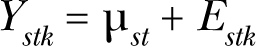
where E(E_stk ) = 0 and var(E_stk ) = $(E_{s k t}) = σ_{s t}^{2}$ . We make the common assumption that the replication variance is equal for each dose, and represent the common variance by $σ_{s}^{2}$ . This assumption is often reasonable since the difference between doses in the low dose region is small, resulting in similar factors contributing to variability in response at low doses.

We use the simple response error model to define the average of μ _st over the three doses, and refer to this average as the ‘true’ response in the low dose range for chemical s given by $μ_{s} = \frac{1}{m} \sum_{t = 1}^{m} μ_{s t}$ . Defining the dose t effect as the deviation from this average, δ _st = μ _st – μ _s , we arrive at the simple model

Y_{s t k} = μ_{s} + δ_{s t} + E_{s t k} .

Such experimental data can be used to test a hypothesis about the true response at low dose, μ _s , versus an alternative hypothesis. For example, assuming response error is normally distributed, a test of the null hypothesis H ₀: μ _s = 0 versus the alternative, H_A : μ _s ≠ 0 results in a t-statistic given by $t = \frac{- 4.67}{3.20}$ , for the data in Table 1. Compared to a t-distribution with three degrees of freedom, the data are inadequate to reject the null hypothesis using α = 0.05, resulting in a p-value of 0.241. Such test results are generated by fitting a one way ANOVA model to the data for the chemical, considering dose to be a fixed effect.

A similar procedure could be used to test the null hypothesis that the true response in the low dose range is the same as control response among all 253 chemicals. For 4 chemicals, since the response for replications at each dose did not differ, the estimate of the residual variance, $σ_{s}^{2}$ , is zero, and hence a test could not be conducted. A histogram of the p-values for the remaining 249 chemicals is given in Figure 1. For 127 chemicals (50.8%), the p-value was less than 0.05, indicating that the null hypothesis would be rejected, supporting the conclusion that the true mean response is not equal to the control response. Among these 127 chemicals, 124 had estimated means greater than the control. If a one-sided hypothesis, i.e. H ₀: μ _s ≤ 0 vs H_a : μ _s > 0 was conducted, the null hypothesis would be rejected for 146 chemicals (58.6%).

These results suggest that there is evidence for many chemicals that the true response is greater than control in the low dose range. Before reaching this conclusion, however, it is important to note that since many hypotheses are tested, there is an elevated risk of falsely rejecting the null hypothesis. In order to control the Type I error, i.e. the probability of rejecting the null hypothesis when the null hypothesis is true, at 5 percent over all the tests, we need to consider test statistics statistically significant only when the p-value is less than 0.05/249 = 0.0002 (using a Bonferroni control for multiple testing (Kutner et al. 2005)). Based on this criterion, only eleven chemicals (4.4%) have test statistics that lead to rejection of the two-sided null hypothesis. Although the mean response exceeds control response for all eleven chemicals, after controlling for multiple testing, there is inadequate data to reject the null hypothesis that the true mean response in the low dose range is equal to the control response for the majority (95.6%) of the chemicals.

The fact that so few hypothesis test results are statistically significant may have been anticipated by some researchers. This result is a consequence of the low power for any individual chemical assay both due to small sample size, and due to the small differences that might be anticipated for the response mean, relative to control. Finally, the results may have been anticipated due to the necessity of controlling for multiple comparisons to maintain the overall false-positive Type I error level at 0.05. This imposes a heavy penalty on tests for individual chemicals, and has a consequence of increasing the magnitude of the differences needed to conclude statistical significance has been reached. Each of these conclusions may have been anticipated by researchers familiar with such methodological issues. The relatively small percentage of chemicals where statistical significance was reached (4.4%) from this perspective could be seen as a confirmation that the analysis was not warranted. Overall, such researchers may conclude that such high through put data are not suitable for learning about response at low doses.

AN ESTIMATION APPROACH TO EVALUATING RESPONSE AT LOW DOSES

We contrast the conclusions from the hypothesis testing approach with conclusions that are developed from an estimation approach. By way of introduction, it should be noted that some researchers (Lehmann 1993, Perlman and Wu 1999, Gigerenzer 2004), openly question the hypothesis testing approach previously described. The estimation approach we describe can be considered to complement the hypothesis testing approach, with a few important differences. We consider a simple approach, using as an estimate of the true response at low doses, μ _s , the estimated mean from an ANOVA model. Since two measures of response at each dose are made, the estimate corresponds to the simple average response at doses in the low dose range. A histogram of these estimates is given in Figure 2 for the 253 chemicals, with a cumulative distribution of the mean response given in Figure 3. The cumulative distribution is constructed by ordering the estimates of response from lowest to highest value, and associating with each response its percentile in the ordered distribution. A plot of the percentile versus the estimate produces the cumulative distribution. The vertical line corresponding to an estimated response of zero would be the expected response if response in the low dose range followed a threshold model. Both Figure 2 and 3 portray elevated average response for the majority of chemicals in the low dose range.

FIGURE 2.

Histogram of Average Response (Percent Difference from Control) in Low Dose Range for 253 Chemicals of ‘WT” Yeast.

FIGURE 3.

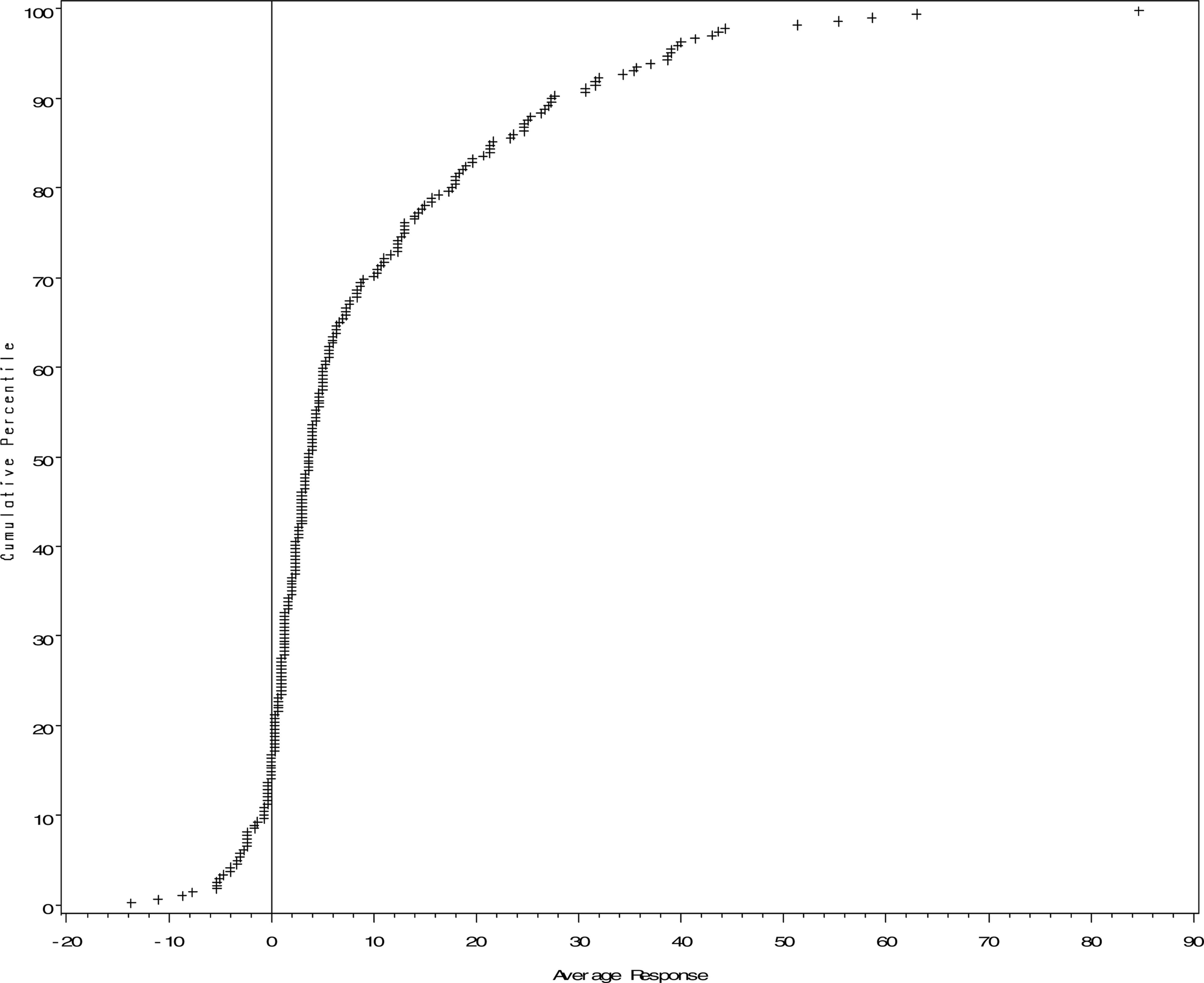
Cumulative Distribution of Average Response (Percent Difference from Control) in Low Dose Range for 253 Chemicals of ‘WT” Yeast.

An aspect of the analysis that is missing from Figures 2 and 3 is a measure of uncertainty in the estimates. Such a measure is typically given in a confidence interval (Neyman 1937). Assuming response error is normally distributed, a 95% confidence interval is defined by two points, $L = {\bar{Y}}_{s} - t_{d f, (1 - α / 2)} S E ({\bar{Y}}_{s}) and U = {\bar{Y}}_{s} + t_{d f, (1 - α / 2)} S E {({\bar{Y}}_{s})}_{s}$ such that P(L < μ _s < U) = 0.95. For example, a 95% confidence interval for the true response based on the data in Table 1 for chemical NSC#1928 based on t _{df,(1–α/2)} = 3.182 is given by the interval (−14.9, 5.5). The width of the confidence interval provides a measure of how large a distance is covered by the central 95 percent of estimates of the true mean from a histogram constructed by multiple, independent samples selected in the same manner.

We can augment the estimate with a confidence interval for each chemical. Is some adjustment needed to account for the fact that multiple confidence intervals are being constructed? If we follow the same logic as in the hypothesis testing setting, it may seem that rather than using α = 0.05 in constructing a confidence interval, we should use a Bonferroni corrected level of α (taken as 0.05/249 = 0.0002) for the confidence intervals. Using such a value of α will result in an ‘adjusted’ confidence interval for chemical NSC#1928 given by the interval (−178, 170). This is a very broad interval, and conveys the impression that there is very little confidence in the estimate −4.67 of true response.

Although the adjustment of the α level for confidence intervals may be sensible when they are used to control the false positive rate (using confidence intervals as a proxy for hypothesis testing), the adjustment of α does not make sense when interpreting the width of a confidence intervals as a measure of the central width of the sampling distribution of the estimator. The fact that this width provides a direct estimate of the sampling distribution width means that multiple comparison adjustments only serve to change the type one error, not adjust for construction of confidence intervals for multiple chemicals. For example, the confidence interval given by (−178,170) is a 99.98% confidence interval, and not a 95% confidence interval that is desired.

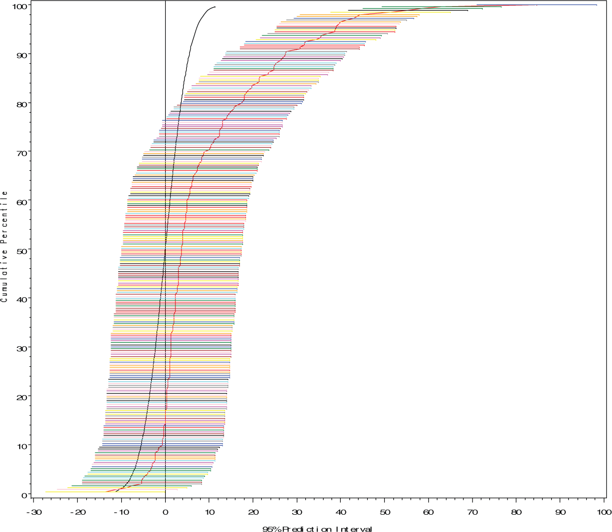
For these reasons, no adjustment to the level of confidence for confidence intervals is needed when summarizing results from multiple chemicals. We can add a confidence interval band to the estimates in Figure 3, resulting in the cumulative distribution of estimates of the true response for 253 chemicals in the low dose range in Figure 4. The endpoints of each horizontal line in Figure 4 represents the lower and upper limits of estimated 95% confidence interval for a chemical, constructed under the assumption that response error is normally distributed. Notice that the confidence intervals appear to be wider at each end of the distribution. This pattern may be associated with the ordering of the sample mean response from smallest to largest value. Also, it is evident that there are some chemicals with very wide confidence intervals, indicating very large standard errors. Some of these large standard errors could be due to outlier values, but the limited data precluded their identification.

FIGURE 4.

Cumulative Distribution of Average Response (Percent Difference from Control) in Low Dose Range for 253 Chemicals of ‘WT” Yeast with 95% Confidence Intervals.

ACCOUNTING FOR RESPONSE ERROR IN ESTIMATING AVERAGE RESPONSE AT LOW DOSES

The results in Figure 4 indicate that wider confidence intervals occur for chemicals when estimated response corresponds to either low or high percentiles. To some extent, response error itself may provide the underlying explanation for the low and high estimates of response. The phenomenon is familiar in many practical problems, such as the observation that baseball batting averages have a broader range early in the season, as discussed by Casella (1985). We provide a similar discussion in the context of estimating the true response in the low dose range.

Suppose a threshold model applies to all 253 chemicals in the low dose range, such that the true response is equal to control response (where the true percent difference from control is zero), but that response is observed with error. An estimate of response corresponding to the average response over measures in the low dose range will not necessarily be equal to zero due to response error. Instead, the average will equal the average response error. Since we have assumed that a threshold model applies to all chemicals, estimating average response in the low dose range will result in 253 independent estimates of average response error. Some of these estimates will be less than zero, while others will be greater than zero. Ordering the estimates from smallest to largest, and plotting them in a cumulative distribution (as in Figure 3) will result in an S-shaped curve that reflects the cumulative distribution of average response error. In this context, estimated response below zero is not a measure of toxic low dose effects, but rather simply an artifact of response error. A similar interpretation applies to estimated response above zero, which do not provide evidence for elevated true response at low doses.

On the other hand, if response error is very small (virtually zero), but chemicals have different true response in the low dose range, then ordering the average response from smallest to largest for chemicals, and plotting the cumulative response distribution will closely represent the true response for the chemicals. In such a setting, the interpretation associated with average response below zero is that there is a low dose toxic effect, and the interpretation associated with average response above zero is that there is a stimulatory effect.

It is possible that both phenomena are present. There is clear evidence of response error since there are different responses for replications of a chemical at the same dose. Similarly, since chemicals are distinct, it is possible that the true response in the low dose region for different chemicals is distinct. Interest is in the true response distribution, not the observed response distribution formed from average estimates for each chemical. The difference between these two distributions is often referred to as regression to the mean (Galton 1886). In reality, since it is possible that both response error and some distribution in the true responses at low dose are present for chemicals, separating these two sources is important for interpretation.

Statistical methods have been developed that can distinguish the true response at low doses from the average response. Such methods are broadly referred to in the context of mixed models as discussed by Brown and Prescott 1999, Bryk and Raudenbush 1992, Demidenko 2004, McCulloch and Searle 2001, and Verbeke and Molenberghs 2000. We briefly describe their application in the context of estimating true response (which we refer to as latent response) in low dose regions.

Consider a list of s = 1, …, N chemicals where assays have been conducted and a low dose range identified. For chemical s, let us represent the latent response in the low dose region by μ _s . We assume that the latent response can not be directly observed, but that the k^th response, which we represent by Y_sk has an expected value equal to μ _s , is given by the model

Y_{s k} = μ_{s} + E_{s k} .

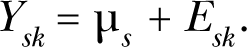
Notice that only Y_sk is observable, not the latent value, μ _s , nor the response error, E_sk . We assume that replicated responses are independent, with variance σ² _s = var(E_sk ). Defining the average latent response over all chemicals as $μ = \frac{1}{N} \sum_{s = 1}^{N} μ_{s}$ , we can represent response via the linear stochastic model

Y_{s k} = μ + β_{s} + E_{s k},

where β _s = μ _s – μ corresponds to the difference between the latent value for chemical s and the average latent value, which we refer to as the effect of chemical s. This model is a fixed effect with only response error considered to be a random variable.

We define a mixed model by considering a subset of i = 1, …, n chemicals to be the result of conceptually selecting a simple random sample of n chemicals. For wild type yeast with three doses in the low dose range, the sample of chemicals is the n = 253 chemicals. Suppose that the order of the chemicals in the sample was determined by selecting a chemical, one at a time from the population, resulting in a sample sequence. Since a chemical could have been selected in any position in the sequence, we represent the chemical effect, β _s , as a random effect, β _i , when the chemical is in position i in a sequence. Once the sequence is known, we know which specific chemical is in position i, where the specific chemical is referred to as the realized random effect. The mixed model replaces the subscript labeling a particular chemical, s, by notation corresponding to selections of chemicals (with the index i) such that

Y_{i k} = μ + B_{i} + E_{i k} .

In this model, B_i is a random effect, the value of which will depend on which chemical is selected in position i in a sample. Prior to selection of the sample sequence, we represent that latent value for the chemical associated with the sample index i by (μ + B_i ). After sampling, this random variable will take on a value equal to the latent value for the selected chemical. In the mixed model, it is commonly assumed that E(B_i ) = 0, since on average, the values of β _s sum to zero, while var(B_i ) = σ², the variance in chemical latent values. We make these assumptions here, noting that they would result if we considered the 253 chemicals as being the entire population of chemicals assessed.

It is possible to predict the latent value corresponding the realized random variable (μ + B_i ). The predictor is called a best linear unbiased predictor (BLUP), and has been widely discussed in the statistical literature (Robinson 1991, Stanek et al. 1999, Stanek and Singer 2004). Representing response for selected chemicals via the mixed model enables predictors of latent values of realized random effects with smaller mean squared error than fixed effect linear model estimators. The gain in accuracy is due to the simultaneous accounting for the uncertainty of both the latent value, and the response error. Relative to the simple estimate of a chemical's latent value based on a sample mean, the BLUP regresses the sample mean, ȳ_i , to an estimate of the overall mean, given by $\bar{Y} = \frac{1}{n} \sum_{i = 1}^{n} \bar{Y}$ (when all chemicals have equal numbers of response), via a shrinkage factor $k = \frac{σ^{2}}{σ^{2} + σ_{e}^{2} / m}$ , where m is the number of measures on a chemical, such that

{\overset{\circ}{Y}}_{i} = \bar{Y} + k ({\bar{Y}}_{i} - \bar{Y}) .

Estimates of the variance components between chemicals, σ², and within chemicals, $σ_{e}^{2} = \frac{1}{N} \sum_{s = 1}^{N} σ_{s}^{2}$ , are substituted into the expression for k to result in empirical BLUPs. The advantage of this approach to estimating latent values for chemicals is that the resulting predictors are more accurate than an estimate of the latent value corresponding to the simple mean. The BLUP for individual chemicals are closer to the chemical average (over 253 chemicals) than simple mean estimates, a factor described as regression to the mean. Figure 5 contains predictors of latent values for chemicals with 3 doses in the low dose range, and accounts for the shrinkage using BLUPs. Note that included in Figure 5 is the cumulative distribution of the average response error distribution, assuming the average response in the low dose range is an estimate of the true control response. The shift of the estimates to the right for the reported data indicates that estimates of the true response in the low dose region are higher than the expected response under a threshold model for most chemicals. The broad interval estimates indicate that the central 95% spread in the distribution of an estimate is approximately ±15%. Overlap of these interval estimates with the vertical like at zero indicates that for many chemical, it is premature to conclude that their true response at low doses is greater than control, while at the same time concluding that it appears for most chemicals, the true response at low doses is greater than control.

FIGURE 5.

Cumulative Distribution of Best Linear Unbiased Predictor of True Response (Percent Difference from Control) in Low Dose Range for 253 Chemicals of ‘WT” Yeast with 95% Confidence Intervals.

DISCUSSION

The apparent conflicting results of hypothesis testing and estimation approaches are directly related to researcher's orientation towards gaining knowledge. Researchers who commonly work in a highly controlled experimental environment are used to designing studies with adequate power to test focused hypotheses and known alternatives. For such researchers, a sequence of such studies leads to measurable progress in research. The experimental design statistical approach has contributed to the steady progress in science. Hallmarks of the approach are the judicious collection of data, reducing both the data collection effort and cost, and the simplicity of statistical analyses for designed studies. The estimation approach does not refute this hypothesis testing paradigm, but provides a different approach in a modern environment where the cost of data collection has diminished, and sequential nature of data collection has been overlaid with the proliferation of very large numbers of relatively small designed studies such as the yeast study, a typical example of a compound screening study.

The estimation approach applied to the yeast study illustrates how data on many diverse chemicals can be assimilated. It provides a snap shot of the multiple studies, retaining important characteristics for individual chemicals such as the confidence intervals reflecting the likely sampling variability of the response. By using models such as mixed models, more accurate estimates of true latent response in the low dose range can be constructed than using conventional fixed effect approaches. The results can be readily summarized using a cumulative distribution of BLUPs of chemicals, and placed in the context of anticipated background response (if true response was equal to zero). The ability to capture this information in a simple figure provides a way of digesting large amounts of study data while retaining the important variability.

It is likely that the number of high through put data sets will increase in the future. As data capture and automated procedures are implemented in more settings, there is more opportunity to learn from the data as long as there are ways of appropriately summarizing the information. Extracting knowledge from such data does not mean solely testing hypotheses, although hypothesis testing has a role in the general process. Visualization of the data is important, and can provide insight. The mixed models accompanied by cumulative plots of best linear unbiased predictors with confidence bands and a plot of anticipated cumulative null distribution can provide an informative summary of large numbers of results.

References

Brown

and Prescott

. 1999. Applied mixed models in medicine. John Wiley and Sons, LTD, New York

Bryk

and Raudenbush

. 1992. Hierarchical Linear Models. Sage Publications. New York

Calabrese

Stanek

EJIII

Nascarella

, and Hoffmann

. 2008. Hormesis predicts low-dose responses better than threshold models. Int J Toxicol 27:369–378

Calabrese

Staudenmayer

Stanek

EJIII

, and Hoffmann

. 2006. Hormesis outperforms threshold model in NCI anti-tumor drug screening data. Toxicol Sci 94:368–378

Calabrese

Staudenmayer

Stanek

EJIII

, and Hoffmann

. 2007. Hormesis and high throughput studies: Crump's analysis lacks credibility. Toxicol Sci 98:602–603

Casella

. 1985. An introduction to empirical Bayes data analysis. Am Stat 39: 83–87

Crump

. 1984. A new method for determining allowable daily intakes. Fundam Appl Toxicol 4:854–871

Demidenko

. 2004. Mixed models: Theory and applications. John Wiley and Sons, New York

Galton

. 1886. Regression Towards Mediocrity in Hereditary Stature. Journal of the Anthropological Institute of Great Britain and Ireland. 15: 246–263

10.

Gigerenzer

. 2004. Mindless statistics. J Socio Econ 44:587–606

11.

Hinkelmann

and Kempthorne

. 2008. Design and Analysis of Experiments: Volume I, II. John Wiley and Sons, New York

12.

Holbeck

and Simon

. 2007. The FHCRC/NCI yeast anticancer drug screen. In: Nitiss

, and Heitman

, (ed) Yeast as a Tool in Cancer Research, pp 347–374. Springer. New York

13.

Kirk

. 1995. Experimental Design. Brooks/Cole, New York

14.

Kutner

Nachtsheim

Neter

, and Li

. 2005. Applied linear statistical models 5th edition. McGraw-Hill Irwin, Boston MA

15.

Lehmann

. 1993. The Fisher, Neyman-Pearson theories of testing hypotheses: one theory or two? J Am Stat Assoc 88:1242–1249

16.

Maxwell

and Delaney

. 1990. Designing Experiments and Analyzing Data. Wadsworth, Belmont, Ca.

17.

McCulloch

and Searle

. 2001. Generalized, Linear, and Mixed Models. John Wiley and Sons, New York

18.

Neyman

and Pearson

. 1933. On the problem of the most efficient tests of statistical hypotheses. Philos Trans R Soc London, Ser A 231:239–336

19.

Neyman

. 1937. Outline of a theory of statistical estimation based on the classical theory of probability. Philos Trans R Soc London, Ser A 236: 333–380

20.

Perlman

and Wu

. 1999. The Emperor's new tests. Stat Sci 14:355–381

21.

Robinson

. 1991. That BLUP is a good thing: the estimation of random effects. Stat Sci 6: 15–51

22.

Rothman

. 1990. No Adjustments Are Needed for Multiple Comparisons. Epidemiology 1 (1): 43–46

23.

Simon

. 2001. Yeast as a model system for anticancer drug discovery. Emerging Ther Targets 5:177–195

24.

Stanek

EJIII

Well

, and Ockene

. 1999. Why not routinely use best linear unbiased predictors (BLUPS) as estimates of cholesterol, Percent Kcal from Fat, and Physical Activity. Stat Med 18:2943–2959

25.

Stanek

EJIII

and Singer

. 2004. Predicting random effects from finite population clustered samples with response error. J Am Stat Assoc 99:1119–1130

26.

Verbeke

and Molenberghs

. 2000. Linear mixed models for longitudinal data. Springer, New York

Predicting Low Dose Effects for Chemicals in High Through-Put Studies

Abstract

INTRODUCTION

A HIGH THROUGH-PUT STUDY OF 2189 CHEMICALS ON 13 STRAINS OF YEAST

DETERMINING A BENCHMARK DOSE

A HYPOTHESIS TESTING APPROACH TO EVALUATING RESPONSE AT LOW DOSES.

AN ESTIMATION APPROACH TO EVALUATING RESPONSE AT LOW DOSES

ACCOUNTING FOR RESPONSE ERROR IN ESTIMATING AVERAGE RESPONSE AT LOW DOSES

DISCUSSION

References