
Abstract
One of the biggest difficulties in telecommunication industry is to retain the customers and prevent the churn. In this article, we overview the most recent researches related to churn detection for telecommunication companies. The selected machine learning methods are applied to the publicly available datasets, partially reproducing the results of other authors and then it is applied to the private Moremins company dataset. Next, we extend the analysis to cover the exiting research gaps: the differences of churn definitions are analysed, it is shown that the accuracy in other researches is better due to some false assumptions, i.e. labelling rules derived from definition lead to very good classification accuracy, however, it does not imply the usefulness for such churn detection in the context of further customer retention. The main outcome of the research is the detailed analysis of the impact of the differences in churn definitions to a final result, it was shown that the impact of labelling rules derived from definitions can be large. The data in this study consist of call detail records (CDRs) and other user aggregated daily data, 11000 user entries over 275 days of data was analysed. 6 different classification methods were applied, all of them giving similar results, one of the best results was achieved using Gradient Boosting Classifier with accuracy rate 0.832, F-measure 0.646, recall 0.769.
Keywords
Introduction
Customer churn analysis plays an important role in all business sectors where customers have a choice between different service providers. A well known fact is that often the costs of existing customers retention are much lower than the costs of attracting new customers, especially it is true for telecommunication companies (Ullah et al., 2019). Thus, in a long-term perspective customer churn problem must be addressed more actively than proper advertisements of company services. There are numerous researches on this topic, however, there is a lack of attention paid to some assumptions such as suitability of different churn definitions. Also, most of the researches do not analyse temporal data, i.e. instead of using call detail records (CDRs) to produce some features and feed the machine learning methods with it directly (Alboukaey et al., 2020) – this limits the analysis to the scope of classification problem alone, however, the success of classification highly depends on the actual knowledge existing in the data.
In the telecommunication industry acquiring a new subscriber costs 16 times more than retaining an existing one (Ullah et al., 2019). The world wide growth of competition in the telecommunication industry along with the maturation of the service market have turned customer churn management into a main challenge within these industries.
Churn prediction problem usually is formalized as a classification problem. More specifically, for a chosen moment t, using the last data before that moment, the method must decide whether the customer will churn after moment t or not, i.e. whether he must be classified as churner. In other words, the binary classification must be performed in order to split customers into 2 classes: churner and non-churner. In other words, such classification means the prediction telling that the customer will not return to the usage of the services from the chosen moment t, however, it can be generalized by requiring to predict churn before the moment of the last customer activity, introducing a time window relative to the last activity in which the churn must be predicted.
The churned customers usually form a minority – the amount of objects we want to detect is small, creating an additional challenge for a proper measurement of classification results and tuning the methods’ parameters. Such data for classification are called imbalanced. As it was pointed out by Chawla (2009) the churn classification data are often imbalanced, i.e. it occurs if objects from one of its categories are 10% or less compared to some other ones. Amin et al. (2016) consider churn detection as a classification problem and focus on the class imbalance problem for the churn detection. Authors used on synthetic dataset and the source of other publicly available datasets were not available, thus, the practical application of results is questionable. This can be seen in other articles as well (Keramati and Ardabili, 2011; Keramati et al., 2014). Thus, the data balancing is important for churn classification, however, in many researches this problem was not addressed.
In most of the researches the churn problem in telecommunications comes down to a classification problem, thus, the accuracy of classification methods defines the wellness of final solution. However, the assumptions used for technical formulation of churn classification problem are often very inaccurate and might lead to bigger solution errors than the classification problem solution itself. One of the main such assumption is the simplified churn definition used for data labelling. This research is dedicated to analyse how does the churn definition (directly affecting labelling rules) affect the churn prediction.
The analysis of the results would let us find out how does the prediction accuracy depend on labelling rules due to different churn definitions. Some of the research questions that will follow from the research are:
There is a wide variety of methods and their combinations were applied to a telecommunication churn prediction. Some of them will be discussed below.
The extensive comparison of different classifiers was done in the research by Adhikary and Gupta (2020) where authors analysed and compared the performance of over 100 classifiers in churn prediction of a telecom company. However, it is important to mention that in the aforementioned research the tuning of different methods was not analysed nor the set hyperparameters were provided – the details were defined by the selected software automatically. Thus, the result of highest accuracy which was given by the Regularized Random Forest classifier is unreliable.
Bose and Chen (2009) have utilized the clustering techniques to improve the decision tree-based churn prediction – clustering was combined with decision trees in such a way that the unsupervised learning technique aided the performance of a supervised learning technique for the classification task of churn prediction.
The other study by Vafeiadis et al. (2015) compares different standard machine learning techniques, the tuning of the hyperparameters is performed, the accuracy level 97% was achieved on the publicly available test data. Data are artificially based on claims similar to the real world (Vafeiadis et al., 2015). Note that the results are highly dataset-dependent, we suppose that in this case the high performance is due to dataset specificity.
Some studies show the possibility to combine multiple methods, for example, De Caigny et al. (2018) develop a new hybrid classification algorithm that uses a combination of decision trees and logistic regression and that is developed to reduce the weaknesses of DT and LR while maintaining their strengths.
Some research is dedicated to alternative classification methods, such as fuzzy classification methods (Azeem et al., 2017). According to the authors, the achieved level of AUC score of 0.68 is high comparing to other authors, however, achieved values above 0.9 can be found in literature (Ahmad et al., 2019). It is important to note that the results might strongly depend on the dataset specificity, the direct comparison between the results of different researchers is very limited, since different researchers use different datasets. It is important to note that (Azeem et al., 2017) ignore the hyperparameter tuning skipping the opportunity to get better results for every method, leading to incomplete comparison between different methods.
The quality of the results might be strongly conditioned by the data preparation algorithms, according to the research by Coussement et al. (2017), the data-preparation technique can strongly affect churn prediction performance. Authors show the improvements of up to 14.5% in the area under the receiving operating characteristics curve (AUC) and 34% in the top decile lift.
In literature, some research that is based on very specific data which is usually not available can also be found. For example, in research by Ahmad et al. (2019) the outstanding 70 terabyte dataset from Syrian company SyriaTel was analysed using Hadoop Distributed File System and Spark engine. According to the authors, the extensive expansion of traditional attributes by some data that use a lot of memory has let them improve the results that otherwise were very poor. However, it should be noted that a lot of data had details about customers. The European Union (EU) regulations on data privacy might not let perform similar analysis in EU countries, since a lot of private data in mentioned research was used, such as exact information of migration between companies for each person. Another note is that according to the information specificity, the matrix with the data was very sparse, thus, the storage of these data could be greatly improved by using compressed matrices. Adwan et al. (2014) analysed the customer movement from one provider to another. However, nowadays, under EU data privacy regulations the implementation of such research would be hard or nearly impossible. Thus, methods in the aforementioned research are not applicable in practice.
In context of the final goal for business, the reason for churn prediction is the possible customer retention; there are researches in which the churn prediction is accompanied by its further application. Ullah et al. (2019) presented the investigation of the existing techniques in machine learning and data mining and proposed a model for customer churn predictions, to identify churning factors and to provide retention strategies. In study by Ahn et al. (2020), there are main concepts for churn loss evaluation presented: Customer Acquisition Cost (CAC), Customer Lifetime Value (CLV); also the feature engineering was discussed. There are successful attempts to include the survival analysis methods into the churn prediction, interpreting the churn retention as a subject survival (Routh et al., 2021), the risks raised due to competing events are used in modelling by a random survival forest.
Literature overview.
Literature overview.
Various machine learning methods are used to determine the churn, as can be seen from the overview in the Table 1. The results obtained in the articles show that the results of the several different methods are good enough. Thus, the efficiency of churn prediction for the actual customer retention might not be bound by the actual (technical) classification performance – the main source of inaccuracy might arise from some assumptions, such as sufficient conditions of churn definition or the assumptions used for the artificial data generation. This is the problem which we are going to address.
In general, there are few most commonly used methods that give a reasonably good results in many researches, moreover, often there were no significant differences between these and some other methods that sometimes perform better in other researches. In our case, several commonly used methods were selected and studied, most of them are tree-based methods.
For example, Adhikary and Gupta (2020) have analysed as many as 100 methods for determining the churn. However, as we have already mentioned, the hyperparameters tuning was ignored. It can be assumed that the hyperparameter optimization was not analysed in the aforementioned research. Thus, it can be considered as a drawback of the considered study.
Another important note can be done based on research by Alboukaey et al. (2020) – the RFM (Recency, Frequency, Monetary) features enabled even such method as Random Forests to perform surprisingly well, however, this method was not among the best ones in other researches. The results without RFM features were much worse in aforementioned research. Thus, in this article we compute RFM features as an important part of dataset for all experiments as well, a detailed description is provided in Section 3.1.
A big amount of flaws can be noted in other researches, which can be seen as research gaps – here we will try to categorize them by providing the appropriate research requirements. From the overview of the results of other researchers, we highlight these requirements which should be fulfilled:
the temporal data is used when the features are derived from actual CDR and/or payment data keeping the information about behaviour dynamics. Data aggregation over the whole period removes the information about the temporal changes in customers’ behaviour leading to the loss of the discriminative ability of the classification methods. Note that the temporal data was not utilized in this research, the most of features lack the information about behaviour dynamics.
the dataset must be not synthetic and the labelling rules and data filtering should be defined, otherwise the usefulness for practical purposes is questionable. The big amount of publicly available datasets are synthetic, the sources of datasets are not properly described, thus, the practical application of results is questionable.
hyperparameter tuning is performed, since methods with default parameter values might perform far from perfect in many cases. The research ignores the hyperparameter tuning skipping the opportunity to get better results for every method, leading to incomplete comparison between different methods.
data balancing is performed as an important part of minority churn class detection. Churn labelling leads to imbalanced data, thus, proper balancing techniques are required to utilize the full power of machine learning methods.
Hyperparameter ranges of classification methods. Here + or − refer to requirement fulfillment or non-fulfillment, accordingly, +/− – means the partial fulfillment of the requirement, the unknown state of the fulfillment of provided requirements is referred as nan.
From Table 2 the lack of the proper attention to the aspects mentioned above can be seen. However, it must be noted that the good results can still be achieved without fulfilling all of these requirements. For example, some of the methods are less prone to the data imbalance problem and might perform relatively well even without balancing, especially if a proper measurement was used (for example, if it is sensitive to the Recall metric such as F-measure). However, according to other authors, these requirements are recommended to be fulfilled and in current research one of the goals is to fulfill these requirements.
Often a churner in the mobile telecommunications is defined as a customer that stops doing revenue generating events during the next 90 days (Alboukaey et al., 2020), while he was active during the observation period. Churn directly affects the profit of the company, thus a customer retention is an important part of company strategy. However, to be able to apply any customer retention, it is necessary to detect the churn event on its early stage, i.e. during the first days of this 90 day period or even before this period has started. In order to estimate the consequences of the churn, it is important to estimate the loss of the profit due to some specific churn event, i.e. churners might have different weights depending on the amount of profit being generated by these customers. However, it is important to note that in most cases the one month period is sufficient to identify the churn case, i.e. the inactivity during 30 days is followed by another 60 day inactivity in most cases. Thus, the definitions of a partial churner as a customer who doesn’t use the services for 30 days might be used in practice. On the one hand, the shorter period lets us label more recent cases, thus it lets a model achieve a faster reaction to the changes in the behavioural patterns. On the other hand, the quality of the possible prediction using shorter time interval might decrease due to possible errors in labels of the churners, i.e. a small portion of partial churners does not fulfill the true churner criteria which means a good machine learning approach will produce a portion of false positives and potentially these false positives could even increase false negatives as well due to the shifts in the model focus while learning from some false data.
The above said implies that it is necessary to find a compromise between relevancy and certainty. This topic has not been investigated before, some authors only mention that in their specific case the churner definition and the partial churner definitions are equivalent in over 80% cases, however, they achieve over 80% accuracy in their predictions using machine learning models, thus it is not clear what is the true accuracy and how does the differences between churner and partial churner affect the final results. On technical level, the aforementioned differences of definitions lead to different labelling rules, thus different training and test data for the classification problem. This is one of the main questions this article is dedicated to.
The main reason behind the churner detection and prediction is the customer retention in order to save the portion of the profit, since in most cases the costs of customer retention are usually much lower than the costs of new user attraction (Barrett, 2003; Lu, 2002). However, the success of retention highly depends on how fast the churn detection was performed. Some authors focus on early churn detection calling it early prediction (Zhang et al., 2016). Therefore, only analysis of retention effectiveness can lead to clues about analysis of suitability and usefulness of different churner definitions, but this is out of scope of the current research. We will assume that the standard definition is the most commonly used definition of 3 months customer activity absence leading to a benchmark rule for labelling the churner. Any other alternative definitions along with their appropriate labelling rules will be considered as approximations of the standard definition, the precision of such approximations is the main topic of the current research.
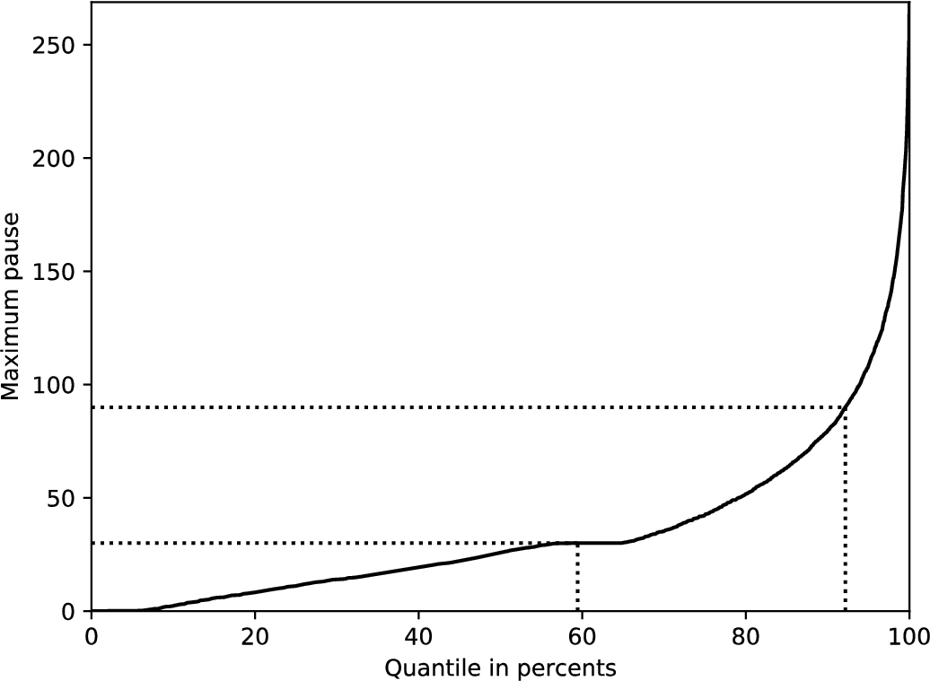
The values of quantiles of maximum pauses during 275 days time interval according to Moremins data.
In Fig. 1, the values of quantiles for maximum pauses per customer are presented. This lets us evaluate the difference of partial churn and churn, more specifically, every customer with maximum pause between 1 and 3 months would mean at least one false positive label if we substitute the churn by partial churn in some specific time window. If we define a churner to be a customer leaving the services forever, then it can be seen that 30 day length interval would let us correctly label up to 59.4% of churners, 90 day interval – would be correct for up to 92.2% of cases. It must be noted that these data are derived from the whole interval, however, at some selected moment there will be only a part of these falsely potentially labelled churners. In other words, the provided estimates show the pessimistic lower bound of correctly labelled churners’ percentage. Thus, the three month period can be seen as quite robust and reliable comparing to labelling in 30 day period. It can be concluded that for the considered data churn and partial churn definitions show how different they can be, despite some authors (Alboukaey et al., 2020) claiming otherwise based on the distribution of churners’ activity during the last thirty days – such analysis can be misleading because the churners form a minority and there might be other customers’ minority group that has a similar activity patterns (e.g. with periodic peaks of activity). The provided rough lower bounds do not prove the suitability or unsuitability of the partial churn definition either. In order to compare the performance of different churner definitions, both definitions with according labelling rules can be used for training the classification algorithm, however, for the final measurement the full churner definition can be used to compare the results of different classification algorithms. Also, it is an open question whether we should consider a churner which stopped using the services for 3 months and have returned afterwards, since it can be considered as churn from competitor services.
Summarizing the said above, there is no perfect churner definition itself and appropriate criteria to define a churner might differ depending on many factors. However, the analysis of suitability and usefulness of different churner definitions is out of scope of the current research, thus, as a standard we will use the most commonly used definition of 3 month customer activity absence and use it as a reference labelling rule. For this research we generalize the churner definition by introducing the labelling rule parameter
The remainder of this paper is organized as follows: the datasets used in this research are described in Section 2, Section 3 provides the method-related information for this study, results are provided in Section 4 followed by discussion in Section 5.
Dataset Overview
The most of the analysed articles have either missing references to the dataset sources or the links to the sources of different datasets are broken. Thus, the amount of publicly available datasets that were used by other authors is quite limited, here we will overview the main of them.
One of the datasets is data from IBM (2020). It is a fictional telco company that provided home phone and Internet services to 7043 customers. The churn column indicates whether the customer left within the last month or not. Other columns include gender, dependents, monthly charges, and information about the types of services each customer has. One of the advantages of these data is column “churn reason”, which we wouldn’t have in real data without additional sophisticated analysis. IBM data have 33 columns and 7043 rows (which is equal to the number of customers).
Amin et al. (2016), Ullah et al. (2019), Xu et al. (2021a) mention a dataset consisting of 3333 instances and 21 attributes, one of which is the churn tag. The links in these articles are not working. However, these data can be found in the Kaggle platform. Dataset is available at (2021).
state – customer state;
total day minutes – total minutes of talk during the day, can be generalized into a value aggregated in other time interval, e.g. total month;
total day calls – number of calls in the day, can be generalized into a value aggregated in other time interval, e.g. month;
total day charge – call charges during the day;
total eve minutes – total minutes of talk last night;
total eve calls – number of calls last night;
total eve charge – charges for calls last night;
total night minutes – night total call minutes;
total night calls – total number of calls in the evening;
total night charge – total charge for calls at night.
Moremins dataset has been taken from a company Moremins. This company is oriented to the niche of customers that migrate between countries, the services are based on cheap calls between different countries, in some of the countries this company has the status of a mobile operator, in others, it has status of a mobile virtual network operator (MVNO). Moremins dataset is not available to public because of the restriction applied on it from Moremins company, since the license was granted for research purposes only. The data is available to researchers in Moremins company and will be available for others after getting the permission from the company (2021). Dataset contains 275 day usage information, the period covered is from 2020-11-10 to 2021-08-12. The data was derived by aggregating Call Detail Records (CDRs) and payment history information. More than 1200000 phone calls and more than 58000 payment records were examined and characterized. The daily aggregation of these data by users yielded 11100 vectors with values of 426 features of daily behaviour.
The attributes of the prepared dataset for the experiments are given in the Table 3. The daily data are calculated for these parameters: call count, the amount of minutes, payment count, the costs of payments.
The aforementioned parameters are calculated for last 90 days of data resulting in 360 features in total.
Structure of the prepared dataset.
Dataset overview is summarized in Table 4.
The churn rate in different datasets. In order to evaluate the imbalanced data problem for different datasets, here we provide the percentage of churned customers among all customers: BigML – 14.49%, IBM – 26.54%, which makes it a slightly imbalanced data, Moremins – 20.21%.
As it can be seen, the imbalance in the considered data is not very high, this will be taken into account later in Section 4.2.
Dataset review.
Feature Extraction
A proper feature extraction might be the key for the performance of machine learning methods. Here we discuss the features used in the current research.
Raw data. Here we present the most detailed form of data feeding the machine learning methods in this research. For that role we have chosen to aggregate the most important parameters for every day per each customer, according to other researches (De Caigny et al., 2018; Alboukaey et al., 2020), the most significant and usually sufficient information is the one which is directly related to the usage of services (minutes, amount of SMS, etc.) or charges for the services (customer payments), thus, a daily data is used and is described as: The sum of minutes from all calls during the day; The amount of calls during the day; The sum of costs of customer payments during the day; The amount of payments during the day.
Thus, we consider this data to create the basis for all future analysis. Next, the appropriate time window must be defined, i.e. how many days must be considered in order to create a sufficient amount of data.
RFM features. As it was mentioned before, the absence threshold for partial churn is 30 days partial, for such labelling in some other researches Alboukaey et al. (2020) RFM-based classification has given one of the best classification results achieving over 90% accuracy.
Compared to usual operators, MVNO clients tend to perform non-regular usage of the services, since clients use services from traditional operators as well. Which means the explicit aggregation of parameters in longer time intervals could give the regularization effect making adding the robustness to the solution.
Recency, Frequency and Monetary (RFM) features are well-known for their suitability for churn modelling (Gupta et al., 2006; Khajvand et al., 2011). These features are the values obtained by aggregation of the considered parameter in the selected time interval in three different ways. Let us assume that we have daily data, i.e. the sums of some parameter for different days, we denote
As it was proposed by Alboukaey et al. (2020), we calculate RFM features in intervals
call count,
the amount of minutes,
payment count,
the costs of payments.
In order to label the data for some time moment t, some amount of future days must be known. This means that if we use partial churn definition to label the data we can do that only for the moment t that is at least 31 days old (compared to the actual real moment). For the RFM feature usage we need the data aggregation in 5 time windows: 4 for RFM features, and one 30 day window RFM features labels RFM features are added to data, the set is split into train and test parts; using the final performance estimation is performed by applying the model on the test part of data labels
As can be seen, for the full analysis of the selected time moment the data from 180 days is needed, the selected time moment to perform the classification is the beginning of 91th day.
Other features. Here we present the list of some simple, yet efficient features suitable for churn prevention, mostly taken from publicly available datasets (Xu et al., 2021a) or based on them: monthly revenue; monthly minutes; state – customer state; payment method; monthly change; percentage change in monthly minutes of use vs. previous three months average; mean monthly revenue over the data collection period; mean number of monthly minutes of use; mean monthly revenue.
Here we provide the sequence of procedures defining the classification algorithm. It must be noted that some standard steps were omitted from discussion since the motivation of their usage is well known and these are done in most of other researches. More specifically we include into the algorithm: data normalization, random oversmapling balancing method, dimensionality reduction method PCA (Principal component analysis). Data normalization is important for variance-based PCA, PCA can increase the performance of some methods such as SVM. Thus, the steps to perform the churn prediction are:
RFM and other feature extraction,
data labelling according to different churn labelling rules,
unsupervised method application: feature vectors’ normalization by standard scaler (division by standard deviation), application of PCA (Principal component analysis),
the construction of classification method based on these steps: random oversampler (churner entries duplicating), the selected method,
execution of Algorithm 1 passing to it data and a method,
saving the metrics.
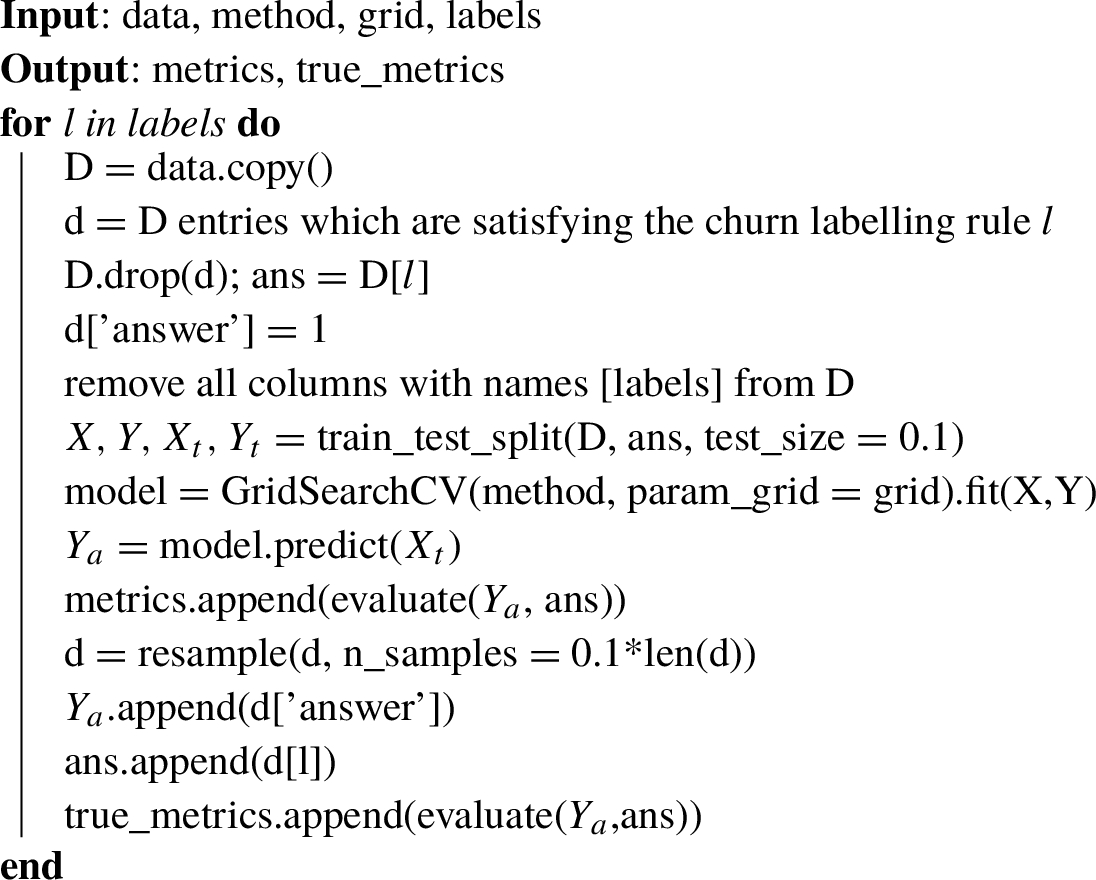
The algorithm for metrics extraction
In Algorithm 1 some of functions reflect the functionality of Pandas dataframes and scikit-learn library, more specifically: method drop() refers to removing the rows (entries); train_test_split randomly splits the data into test and training/validation samples with the given proportion (0.1 to the test part); GridSearchCV iterates through all possible combinations of the given ranges of parameters; resample refers to the random sampling from the given set of entries at the given proportion, i.e. it leaves 0.1 of the initial rows to sustain the constant proportion of removed and total entries between the initial and test data.
Also, the true metrics concept is indirectly present in Algorithm 1, it will be described in details in Section 3.4.
Taking into account the results obtained by other authors, we notice that the methods based on the decision tree give a good enough result. GradientBoostingClassifier (GBC) is a stochastic gradient boosting algorithm, which was proposed by Friedman (2001, 2002). The weak learner of this method is a decision tree. On each iteration, trees are fit on the negative gradient of the loss function evaluated at the previous iteration. XGBClassifier (XGBoost) was proposed by Chen and Guestrin (2016). This model grows trees level-wise. It was developed as a method for computation speed and performance. It is state-of-the-art in many articles. LGBMClassifier (LGBM) – a gradient boosting model (Ke et al., 2017). This model grows trees leaf-wise. It chooses the leaf which is predicted to give the largest improvement for the loss function. RandomForestClassifier (RF) was proposed by Breiman (2001). This method creates a forest of random trees. L. Breiman minimized the generalization error for forests, because the number of trees in the forest increases. KNeighborsClassifier (KNN) was first developed by Fix and Hodges (1951). The idea of this method is to assign classes to new data (test data) on the basis of data already classified (learning data). SVM – supervised classification method for classification in two groups. SVM was proposed by Cortes and Vapnik (1995). The training data are divided in the high dimension feature space so that the distance between the classes is the greatest. New data (test data) is displayed in the same space. The assignment of test data is based on which side of the gap it is displayed.
We find a lack of description of different metrics’ importance in other researches, thus, here we will fill this gap by discussing different metrics in the context of the churn problem.
Accuracy. Accuracy is the most common metric to measure the performance of classification method. What it lacks is the sensitivity for imbalanced data, i.e. if, for example, there are 10% of churners in the data, and there will be no single churner classified, the accuracy will still show value 0.90 which is usually a good result in the case with balanced data. For churn prediction the focus must be made on churners, the minority of objects, so the accuracy doesn’t show the performance very well.
Recall. Recall or true positive rate (TPR) is calculated as
Specificity. Specificity or true negative rate (TNR) is calculated as
Precision. Precision or positive predictive value (PPV) is calculated as
Balanced accuracy. Balanced accuracy is a compromise between recall and specificity, more specifically, it is an average of the aforementioned two metrics
F-measure. F-measure has the same motivation behind it as the balanced accuracy has, but the counterpart of recall is selected to be the precision which is far more suitable to describe the success of minority prediction. Moreover, attention should be paid to the fact that we are talking about rates, so the significance of the changes of absolute values depend on the values themselves, e.g. decrements of 0.1 have a more dramatic effect for value 0.11 than for value 0.9. In such situations a more appropriate way to find a compromise is to use harmonic mean instead of arithmetic average. Thus, F-measure is the harmonic mean of precision and recall
AUC. The aforementioned metrics are calculated using a finally tuned and fixed classification method, however, often methods give you the estimations of likelihood of some object being belonged to one or other class, the final classification is performed by selecting discrimination threshold which must be stepped over in order to assign the object to some class. This means, that, for example, you can sacrifice the accuracy for a bigger recall if you shift the discrimination threshold for the final decision. In other words, after the learning process is finished, you can create a series of classification algorithms by choosing different thresholds and draw the ROC curve describing the dependence of TPR on FPR, both values will increase from 0 to 1 forming a curve. The area under ROC curve (AUC) is a good way to estimate the overall machine learning technique independently of discrimination threshold. The closer AUC value to 1 – the better, AUC equal 0.5 means the method’s performance is similar to random classifier.
True metrics. In the context of the current research there is a need to distinguish between the classification metrics and the actual metrics in terms of the true (full) churn definition. The reason is the partial churn definition and generalized definitions which let the churner be labelled based on the inactivity time interval which is less than 3 months. However, it is done with the intention to predict the churner based on the full churner definition assuming that the differences between aforementioned definitions are small.
For correct formulation of classification problem we must remove the entries for which the answer is already known. It is assumed that the definition itself is changed to an alternative one with other labelling rule, so if the object fulfills this definition the prediction is not needed, the answer is known. Such removal of the entries is an exact representation of what is done in other researches, Alboukaey et al. (2020) excluded inactive customers for the last 30 days. I.e. in the training data there should be no customers who are inactive for the last
Therefore, to unify the metrics for different churn definitions we introduce the true metrics concept – before the final measurement, the entries, which where excluded due to decreased time interval in labelling rules, must be returned to the dataset, such objects must be labelled as churners.
Experimental Results
Data Preparation
The labels defining different labelling rules for different churn definitions.
The labels defining different labelling rules for different churn definitions.
As it was mentioned in Sections 1.3 and 3.4, the churn definition, which is used for labelling, affects the dataset. A single parameter can be used to describe different labelling rules for different churn definitions used in the current research – the amount of days of customer absence
Churner – the churner according to the standard 90 day absence definition,
Churner4 – the label according to a partial churner definition which is often used as an alternative due to many reasons and assumptions,
Churner1, Churner2, Churner3, Churner4 – the labels used to describe the compromise between the standard (full) and partial churner definitions,
Churner5 – the label used to investigate the extreme case with a very short churner detection window of 15 days.
Note that in order to label the data, additional 90 days from the future were used, expanding the actual time interval used to create the dataset from 275 to 365 days, last 90 of which were used only for labelling.
The explored hyperparameter ranges in current research are presented in Table 6.
Hyperparameter ranges of classification methods.
Hyperparameter ranges of classification methods.
Hyperparameter values for Moremins dataset are presented in the Table 15 and for other datasets in Table 8. The appropriate parameters were selected by trying all possible combinations using the Grid search method, as a comparison criterion F-measure was used.
As it was already presented in Section 2, the imbalance in the considered data is not very high. Thus, metrics for imbalanced data, such as F-measure, should not be blindly considered as the only right way to seek for an optimal solution. It is possible to optimize the F-measure metric at the cost of Accuracy via thresholding techniques or even the usage of special loss functions, however, the optimality of results obtained in that way can be still questionable as there is no single perfect way to measure the performance of the methods. Thus, the approach used in this research is to let methods converge using loss functions which are known to be most suitable for according methods, i.e. default ones, however, to use F-measure to perform the final selection of combination of hyperparameters.
Comparison of different methods for different datasets is presented in Tables 9–13.
Results of different datasets using different methods.
Results of different datasets using different methods.
As it can be seen from Table 7, the achieved accuracy score for dataset BigML is close to the values which were presented for this particular dataset by other authors, which in most cases are between 0.91 and 0.98 (Xu et al., 2021b; Śniegula et al., 2019), as for IBM dataset, its accuracy values can be found in literature to be between 0.69 and 0.80 (Singh et al., 2021; Pamina et al., 2019). However, in some sources there is a lack of information about the F-measure scores which were used in the current research as the criterion to choose parameters, thus, in this research, a bit of accuracy might be sacrificed to achieve a better F-measure. Thus, from now we assume that the achieved results along with the quality of the selected methods are similar to the ones existing in other researches. In Table 8 the used parameters are presented.
Hyperparameters of model for different datasets.
Results of dataset with different churn labelling rules using GBC.
Results for Moremins dataset with different churner labelling rules using XGBoost.
Results for Moremins dataset with different churner definitions using LGBM.
Results for Moremins dataset with different churner definitions using RF.
Results for Moremins dataset with different churner definitions using KNN.
Results for Moremins dataset with different churner definitions using SVM.
Hyperparameters of methods for Moremins dataset.
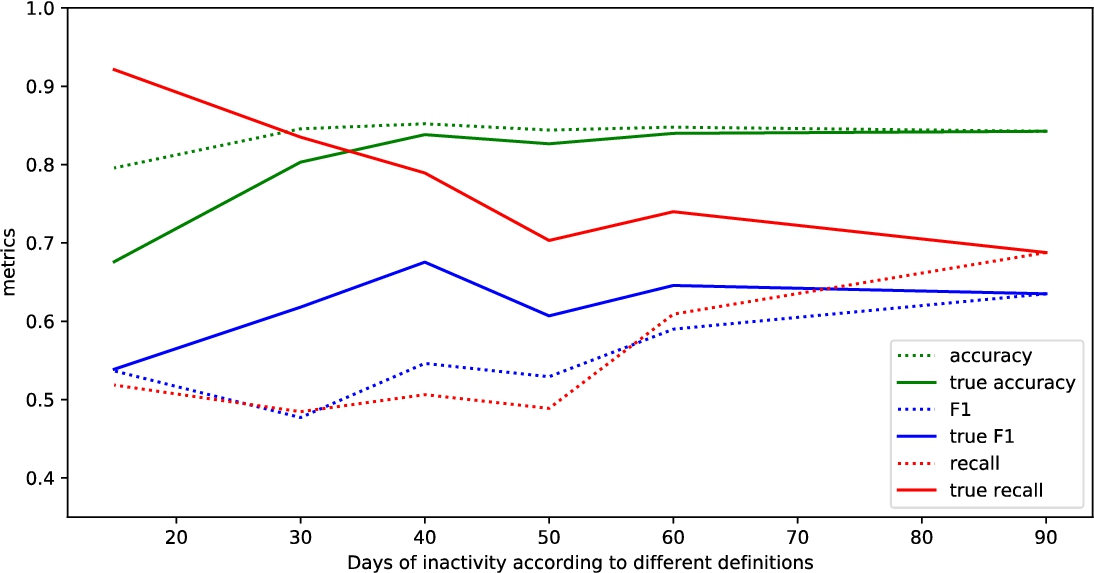
The results of different metrics with different churn labelling rules using different methods are provided in Tables 9–14. In these tables we provide the metrics values for different methods with different labelling rules, for each rule there are two different metrics sets presented: the standard one which is used in all other researches and the True metrics (which were introduced in Section 3.4). The general note on the provided tables is that different methods show similar performance in many cases. Some special cases of exceptional values might be related to the specificity of the data in the provided dataset, thus, next, the attempt to provide general insights of tendencies in the results will be performed.
The dependency of results on the amount of days of customer inactivity
As the
As it can be expected, true Recall decreases, true Specificity increases. There are some exceptions. The Specificity with labelling rule Churner2 and Gradient Boosting Classifier method worked surprisingly well due to some reasons that are hidden from the researcher, such as better suitability of the provided set for convergence. As it can be seen from Table 15, it takes the highest N-estimators and different parameters than with other churn labelling rules leading to a better result. The same stands for Recall for these cases: XGBoost with Churner4, LGBM with Churner2.
True precision values depend on the precision of classification and the rate of churners among the additional entries. More specifically, the low values of precision with labelling rule according to full churner definition mean more chances to be improved by the big rate of true positives among the additional entries. The overall picture from the Tables is clear – the precision decreases together with
True accuracy parameter decreases, more specifically, partial churner (with corresponding label Churner4) comparing to full churner results in these accuracy drops: 0.089 for GBC, 0.072 for XGBoost, 0.039 for LGBM, 0.049 for RF, 0.08 for KNN, 0.076 for SVM.
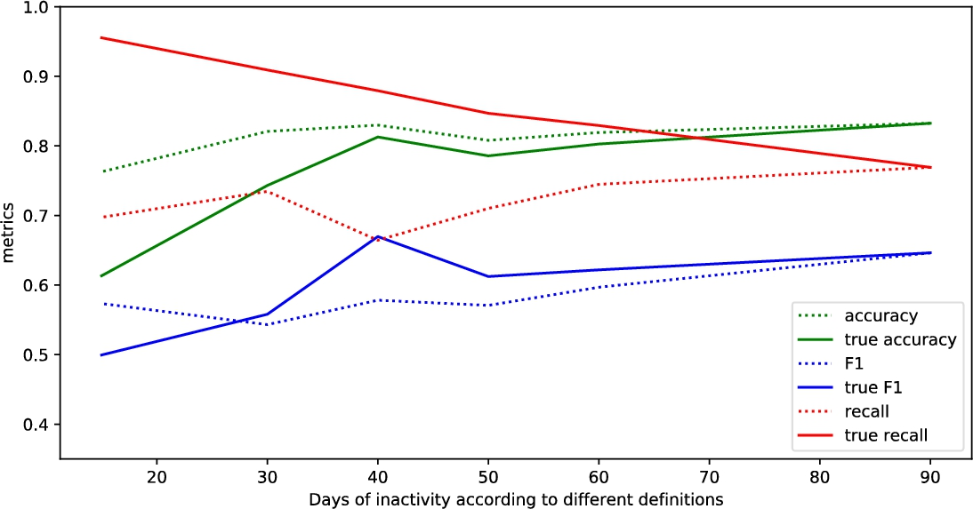
In Figs. 2–7 there are presented results from Tables 9–14 for Recall, Accuracy and F-measure metrics. The interesting observation is that the high recall with lower
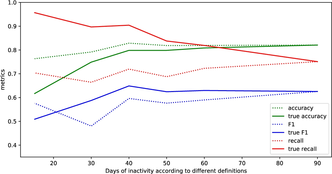
The dependency of results on the amount of days of customer inactivity
The dependency of results on the amount of days of customer inactivity
The dependency of results on the amount of days of customer inactivity
The dependency of results on the amount of days of customer inactivity
The dependency of results on the amount of days of customer inactivity
In this research we have mainly focused on tree-based classification methods, as these performed well in many other researches in the context of churn prediction for telecommunication data. These methods were applied to publicly available datasets, partially reproducing the results of other authors. There was no intention to improve the results of other authors directly via methods and their usage development, the main focus was made to investigation of churn definitions and their according labelling rules suitability or unsuitability in the context of churn prediction for telecommunication companies. For this purpose, the data from Moremins company was used, this company specializes on MVNO services.
Due to imbalanced data nature, one of the main selected metrics of performance in this research is F-measure which represents the goal of churn detection very well, it is derived from both precision and recall which are both oriented towards positive answer estimations, i.e. it fits well the churn minority detection. However, the imbalance in the considered data is not very high, since the churn rate is 20.21%, thus, it was decided to not use it for method thresholding in order to optimize this metric, but F-measure was used to select the best combinations of parameters during the Grid Search procedure which was used to tune the model.
According to full churn definition, the best F-measure 0.646 was achieved with GBC method with accuracy 0.832, the best accuracy was achieved using Random Forest classifier with F-measure 0.614. Note that in similar research by Alboukaey et al. (2020) one of the best results was achieved using RFM-based Random forest classifier with F-measure 0.525. Thus, we can conclude that Random Forest Classifier supported by RFM features extraction gives reasonably good results despite being considered less advanced method than some other methods.
The results have shown that the reduction of the time interval used for churn labelling rule from 90 to 30 days results in a drop of machine learning performance rates: up to 0.089 for accuracy and 0.088 for F-measure in case of GBC method. However, an interesting observation can be made if that period of 30 days is extended to 40 days – in this case the losses of accuracy are much lower and F-measure greatly increases due to raise of Recall, which is expected due to additional positive answers in the data. However, this effect might be related to Moremins data specificity, so in order to generalize the conclusions, it is necessary to verify these results with other datasets.
It is important to note that all publicly available datasets do not have temporal data, such as daily activity of customers. Moreover, there are many datasets that were created synthetically, production steps of the rest datasets are unknown or are hard to find, the definitions and labelling rules used in them are not clear either. In fact, this lack of knowledge for the nature and derivation of the data related to churn in telecommunication industry raise many questions of data applicability in practice. All the aforementioned data issues create a challenge to make strong and general conclusions with fact verification. However, the methodological steps provided in current research contribute to further development of the general principles of churn prediction for telecommunication companies.
Summarizing the said above, this research makes step forward from methodological point of view for prediction of churn in telecommunications. We showed that omitting the inaccuracies in churn definition might lead to misleading results, small inactivity interval solves a problem which differs a lot comparing to original problem. The accuracy in other researches is better due to some false assumptions, i.e. labelling rules derived from definition leads to a very good classification accuracy, however, it does not imply the usefulness for such churn detection in the context of further customer retention.
The findings in this study raise other questions that might be considered as research gaps: Do companies actually need a binary classification of churners, if the result is sensitive to the assumptions that look natural? Some sort of alternative classification generalization could be considered. Especially it can be true since nowadays changing operators is easy, also new eSIM technology possibilities appeared, the loyalty to some services of companies might be much more fuzzy than it was a couple of decades ago. The changes of behavioural patterns might greatly affect the proper classification procedure, thus data getting old can significantly affect the results, however, in most studies even the time period is not presented. I.e. even the fact of year season might greatly affect the behavioural patterns of clients, for example, in winter due to Christmas and other socially important events the behavioural pattern might differ a lot comparing to periods during summer time.
The performed research has let us answer relevant questions and make conclusions, some of which are following:
If the full churner definition must be avoided for different reasons, such as changes in user behavioural patterns, then the definitions based on 40 day inactivity interval can be a reasonable compromise to achieve reasonably good prediction accuracy, the main sources of errors in such case will likely be the classification problem solution.
According to the full churn definition, the best F-measure 0.646 was achieved with GBC method with accuracy 0.832, the best accuracy was achieved using Random Forest classifier with F-measure 0.614.
In terms of F-measure True metric, the best result was achieved with LGBM method using Churner3 label according to definition based on 40 day interval absence. It is important to note that labelling according to full churner definition gave worse F-measure result, although accuracy is better.
The most significant differences in True and standard metrics due to differences of churn definitions can be seen in cases of usage of LGBM and RF methods. For illustration, as a reference we will use Churner4 label derived from 30 day churn definition as it is done in other researches. For LGBM, the Recall metric standard one equal to 0.484, True – 0.835, F-measure standard and True are equal to 0.477 and 0.618, accordingly. There are similar big differences in case of RF method: the Recall standard and True metrics are equal to 0.406 and 0.781, accordingly; the F-measure standard and True metrics are equal to 0.446 and 0.587, accordingly.