Sage Journals: Discover world-class research

Abstract

A large number of modern mobile devices, embedded devices and smart home devices are equipped with a voice control. Automatic recognition of the entire audio stream, however, is undesirable for the reasons of the resource consumption and privacy. Therefore, most of these devices use a voice activation system, whose task is to find the specified in advance word or phrase in the audio stream (for example, Ok, Google) and to activate the voice request processing system when it is found. The voice activation system must have the following properties: high accuracy, ability to work entirely on the device (without using remote servers), consumption of a small amount of resources (primarily CPU and RAM), noise resistance and variability of speech, as well as a small delay between the pronunciation of the key phrase and the system activation. This work is a systematic literature review on voice activation systems that satisfy the above properties. We describe the principle of various voice activation systems’ operation, the characteristic representation of sound in such systems, consider in detail the acoustic modelling and, finally, describe the approaches used to assess the models’ quality. In addition, we point to a number of open questions in this problem.

Keywords

voice activation keyword spotter hidden markov models acoustic model neural networks

1 Introduction

The voice activation task has been attracting both research and industry for decades. Since the task of formulating an algorithm to determine whether a code phrase has been uttered in an audio stream is difficult, it is not surprising that heuristic algorithms and machine learning methods have long been used for the voice activation problem.

The history of voice activation models has gone through several important stages in parallel with solving a more general problem of automatic speech recognition. We would like to highlight the following important moments: the beginning of the use of hidden Markov models back in 1989 (Rohlicek et al., 1989), the use of neural networks since 1990 (Morgan et al., 1990, 1991; Naylor et al., 1992), the use of pattern matching approaches, in particular, dynamic time wrapping (Zeppenfeld and Waibel, 1992) optimization of a loss functions specific to a voice activation (as opposed to the common metrics such as accuracy and similar; this enables the system to become more attractive in terms of user experience) (Chang and Lippmann, 1994; Szöke et al., 2010), attempts to get rid of a garbage model (Junkawitsch et al., 1997), building systems of voice activation for non-English languages such as Chinese (Zheng et al., 1999; Hao and Li, 2002), Japanese (Ida and Yamasaki, 1998), Persian (Shokri et al., 2011), construction of discriminative systems (Keshet et al., 2009; Tabibian et al., 2011, 2013), publications describing voice activation systems in mass products (Chen et al., 2014a; Gruenstein et al., 2017; Guo et al., 2018; Wu et al., 2018), as well as publishing open datasets to compare different approaches (Warden, 2018).

Voice activation systems can be applied in various areas: telephony (Shokri et al., 2013; Szöke et al., 2010), crime analysis (Kavya and Karjigi, 2014), the assistance systems in emergency situations (Zhu et al., 2013), automated management of airports (Tabibian, 2017) and, naturally, personal voice assistants, built-in mobile phones and home devices (Gruenstein et al., 2017).

The problem of voice activation is closely related to the problems of automatic speech recognition and spoken term detection. In ASR, the task is to find the most likely sequence of words spoken in the audio recording, whereas in voice activation we need to find only a predetermined set of words or to indicate that such a word/words was/were not spoken. Of course, being able to solve the problem of ASR can easily solve the problem of voice activation, but at the moment most of the speech recognition systems consume an unacceptably large amount of resources for voice activation.

Spoken term detection is a search for a given phrase (and this phrase may vary depending on the request) in a static set of audio data. In voice activation, the phrase is fixed, but the audio data is delivered in real time. Therefore, you can use offline methods in spoken term detection, such as bidirectional neural networks or audio pre-indexing.

Despite the differences in these problems, approaches and ideas often overlap. For example, audio data representation, decoding methods or architecture of acoustic models. Additional requirements may apply for voice activation systems. For example, responding only to a keyword that was addressed to the system, but not to the same keyword spoken in the conversation (wake-up-word detection) (Këpuska and Klein, 2009; Zhang et al., 2016); responding only to a keyword spoken by a registered user (Gruenstein et al., 2017; Manor and Greenberg, 2017; Kurniawati et al., 2012).

In this paper, we will focus primarily on voice activation systems that can be used in embedded systems, in particular, mobile phones. Such systems must satisfy the following properties:

•
high recall of finding the keyword (to build a voice interface, you need to be sure that you can start the voice interaction; with a low recall, the user will have to start the interaction in a different way),
•
a small number of false positives (since the voice activation system is always on, a large number of false positives is unacceptable: this causes a waste of device resources, distracts the user’s attention and potentially reduces security),
•
the ability to work entirely on a limited resource device (firstly, continuous forwarding of audio data to remote servers is impossible due to prohibitively high requirements for resources and communication coverage, and secondly, it is undesirable from the user privacy’s point of view),
•
consumption of a small amount of resources (due to the previous property, consuming a large amount of resources will lead to rapid battery depletion and slow operation of other processes),
•
noise resistance and variability of speech,
•
a small delay between the utterance of the keyword and system activation.

We will call systems that satisfy these properties small-footprint keyword activation systems, similar to Chen et al. (2014a). Thus, some papers that suggest the operation of the system in milder conditions (for example, not in real time) were omitted from the study.

Previously, there were reviews of voice activation systems (Bohac, 2012; Rohlicek et al., 1993; Morgan and Scofield, 1991), but there is some outdated information (due to rapid development in the area). Also, as far as we know, our work is the first systematic literature review on the subject.

This work has the following structure. In Section 2, we describe the structure of a typical voice activation system, and will help to state the research questions which we aim to answer in this work. Next, in Sections 3, 4, 5, 6, and 7, we provide the answers to these questions. In Section 8 we describe approaches that are difficult to relate to the typical system described in 2. Finally, in Section 9, we summarize the study and describe possible areas for further work.
2 Structure of Voice Activation System

As described in Section 1, voice activation systems have come a long way. One way to study and compare approaches is to provide the model of a system and to compare the individual components of the model. Most voice activation systems (especially modern ones) consist of the following parts:

•
feature extraction from audio data (to represent audio data in format acceptable to machine learning models and obtain input data that has enough information to solve the problem),
•
application of the acoustic model (a system that generally computes the probability of acoustic observations, which often comes down to computing
$P (u | O)$ $ P(u|O)$
, where u is an acoustic unit and O are acoustic observations),
•
decoding: the process of determining the state sequence with the reference to acoustic observation and acoustic model in order to determine whether a keyword has been uttered or not.

For example, Chen et al. (2014a) describe voice activation systems that apply an acoustic model specified by deep neural network to extracted Log Mel-filterbank (feature extraction) and decide whether the keyword was uttered by smoothing deep neural network outputs and comparing them with a threshold (decoding).

Of course, not all the possible voice activation systems are well described by the scheme. For instance, in pattern-matching approaches it is hard to separate acoustic model and feature extraction. Discriminative spotters would be another example. We will discuss these and other systems in more detail in Section 8. Nevertheless, even in these systems it is always possible to point out the feature representation of the audio or some kind of the acoustic model.

This systematic literature review aims to summarize information available in studies about voice activation systems for embedded devices by answering the following research questions: 1.
What acoustic features are used?
2.
What types of acoustic model are used?
3.
What acoustic units are used in acoustic modelling?
4.
What types of decoder are used?
5.
What metrics are used to evaluate systems’ quality?

3 Feature Representation

Sound is a continuous physical phenomenon of mechanical vibration transmission in the form of an acoustic wave. However, most machine learning models do not accept continuous data as input. Thus, the extraction of features from the audio recording has two main goals:

•
representing audio in a way that would be suitable to machine learning methods,
•
the preservation of the largest possible amount of information needed to solve the problem (i.e. finding keywords) and the exclusion of the largest possible amount of information irrelevant to the task (“noise” such as background sounds or the variability of speech).

Most voice activation systems use an approach similar to speech recognition systems (Hinton et al., 2012).
1.
The original recording is segmented in possibly overlapping frames.
2.
In each frame, a numerical vector that describes the behaviour of the sound at this time interval is computed (usually, this vector is computed using the discrete Fourier transform). Let’s say that this vector has dimension
$n_{f}$ ${n_{\mathrm{f}}}$
.
3.
The resulting numerical matrix of the size
$T \times n_{f}$ $ T\times {n_{\mathrm{f}}}$
is used as the result of feature extraction (where T is the number of frames).

Thus the audio data can be viewed as a 2D-image or a time series. The specially selected transformation used in the second step is responsible for extracting the most discriminative features for the voice activation task.

Of course, not all the systems go this way. For example, Kumatani et al. (2017) use raw waveform (without any selected transformations), and Lehtonen (2005) develops a specific digital signal processing pipeline.

Sometimes, feature quantization is used to increase the speed of operation, reduce consumption or for specific algorithms (Feng and Mazor, 1992).

Mel Frequency Cepstral Coefficients (MFCC) is the most frequently used feature type in the studied sources. It is calculated in the following way:
1.
The audio is segmented into short frames (popular choice is to have 25 ms segments with the overlap of 10 ms).
2.
For each frame the periodogram estimate of the power spectrum is computed. This is similar to the way human cochlea processes the information (different nerves fire signals depending on the frequency of the audio). To get the estimate, first Discrete Fourier Transform of each frame is computed via:
$\begin{matrix} S_{j} (k) = \sum_{n = 1}^{N} s_{j} (n) h (n) exp (\frac{- 2 i π}{N} k n), \end{matrix}$ \[ {S_{j}}(k)={\sum \limits_{n=1}^{N}}{s_{j}}(n)h(n)\exp \left(\frac{-2i\pi }{N}kn\right),\]
where j is the frame number,
$1 ⩽ k ⩽ K$ $ 1\leqslant k\leqslant K$
, K is the DFT length,
$h (n)$ $ h(n)$
is an N sample long analysis window (e.g. Hamming window),
$s_{j} (n)$ ${s_{j}}(n)$
is the n-th sample of the j-th frame. After that, the periodogram estimate is computed by:
$\begin{matrix} P_{j} (k) = \frac{1}{N} {| S_{j} (k) |}^{2} . \end{matrix}$ \[ {P_{j}}(k)=\frac{1}{N}{\big|{S_{j}}(k)\big|^{2}}.\]

3.
Apply the Mel-filterbank to the power spectra summing the energy in each filter. The Mel scale relates perceived frequency. Human ear is more sensitive to small changes in low frequencies than in the higher spectra. In order to convert frequency f to Mel scale, the following formula is used:
$\begin{matrix} M (f) = 1125 ln (1 + f / 700) . \end{matrix}$ \[ M(f)=1125\ln (1+f/700).\]

4.
The logarithm of filterbank energies is taken. This also relates to human perception: the loudness does not change linearly with the energy. Logarithm is good approximation and also it allows to perform channel normalization with simple subtraction (e.g. cepstral mean normalization).
5.
Discrete cosine transform is applied. This is done to decorrelate the filterbank energies which were computed with overlapping filters.

Although the vast majority of articles use Log Mel-filterbank (fbank) or Mel Frequency Cepstral Coefficients or their derivatives, the question arises whether this approach is universal, i.e. suitable to all situations. It turns out that this is not the case, for example, during the development of voice activation systems for the Japanese (Ida and Yamasaki, 1998), the prosodic information had to be used to achieve acceptable quality, as MFCC did not give sufficient results. This situation happens with some other languages, too (Zheng et al., 1999).

Among the common techniques, one can use stacking (concatenation of feature vectors from the current and neighbouring frames) and the calculation of delta or derivatives (i.e. the calculation of a discrete time derivative using features from neighbouring frames). Also, a mean normalization or a variance normalization is often used. In the cepstral range, this transformation is usually abbreviated as cmvn.

For a detailed description of the mentioned features, you can refer to the relevant articles or reviews (Giannakopoulos, 2015). The visualization of some of the features for the phrase “Hello, world!” is shown in Fig. 1 and is computed using the framework for speech recognition kaldi (Povey et al., 2011).

Fig. 1.
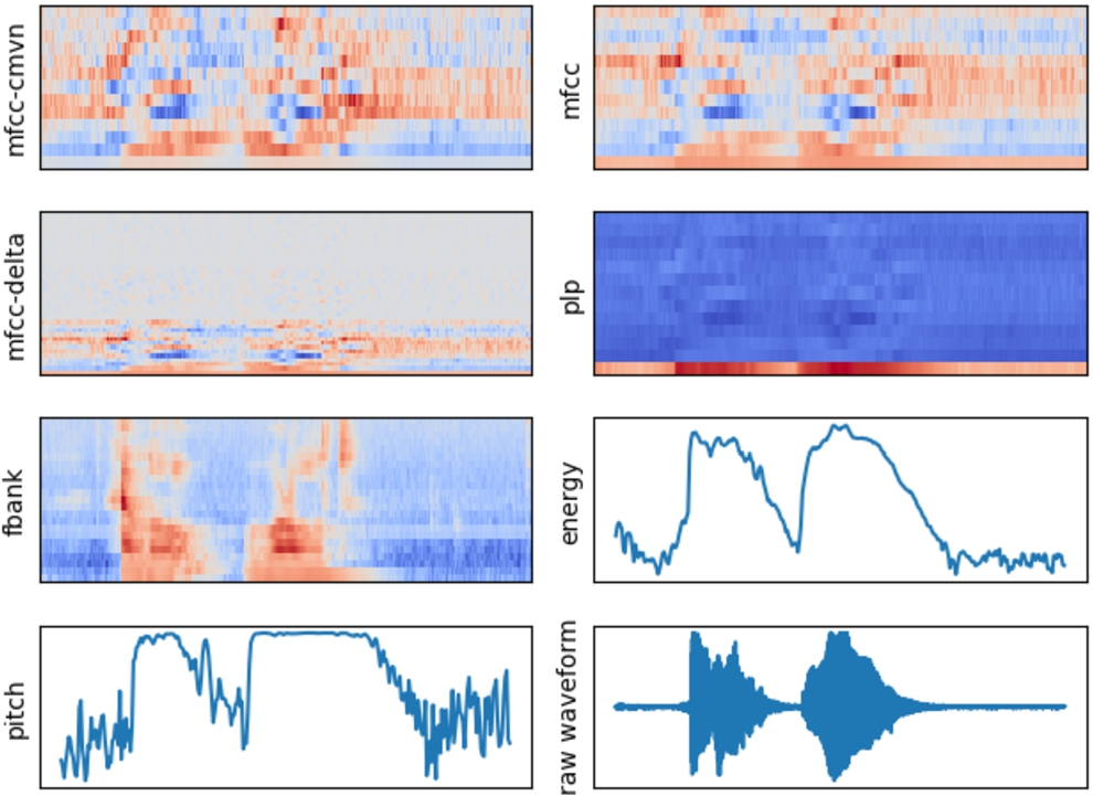
Feature visualization for audio file with “Hello, world!” pronunciation.

The acoustic features used in studied sources are presented in Table 7, in Appendix A. The number of times these features were used in the sources is presented in Table 1.

Table 1
The umber of times acoustic features and transformations were used in studied sources.

Acoustic features and transformations Number of sources

Mel Frequency Cepstral Coefficients 25

Derivatives or deltas 24

Log Mel-filterbank 9

Mean/variance normalization 8

Linear predictive coding 6

Energy or log-energy 5

Fourier transform 4

Stacking, perceptual linear prediction 3

Gain normalization, prosodic information, linear discriminant analysis over MFCC autoregressive moving average, spectral entropy, spectral flatness burst degree, bisector frequency, formant frequencies, feature space Maximum Likelihood Linear Regression, raw waveform 1

4 Acoustic Model

Acoustic features and transformations	Number of sources
Mel Frequency Cepstral Coefficients	25
Derivatives or deltas	24
Log Mel-filterbank	9
Mean/variance normalization	8
Linear predictive coding	6
Energy or log-energy	5
Fourier transform	4
Stacking, perceptual linear prediction	3
Gain normalization, prosodic information, linear discriminant analysis over MFCC autoregressive moving average, spectral entropy, spectral flatness burst degree, bisector frequency, formant frequencies, feature space Maximum Likelihood Linear Regression, raw waveform	1

The task of the acoustic model is to model acoustic properties of the selected acoustic unit. For example, an acoustic model can provide a probability distribution over the vectors of MFCC-features when a certain word is pronounced. Practically, the acoustic model is used to compute

P (S | u)

$ P(S|u)$

, where S – sound and u is some acoustic unit.

Often it is more natural or easier to compute

P (u | S)

$ P(u|S)$

, and then get

P (S | u)

$ P(S|u)$

via Bayes theorem. Especially often this technique is used in conjunction with Hidden Markov Models (HMM).

The most common acoustic model for voice activation is built as follows. The set of HMM states is logically divided into two parts: a part that represents audio event of keyword pronunciation and a garbage model (a model of the rest of the sound: noise, background speech, actual voice request). Figure 2 shows a typical HMM used in Amazon’s spotter for the keyword “Alexa”.

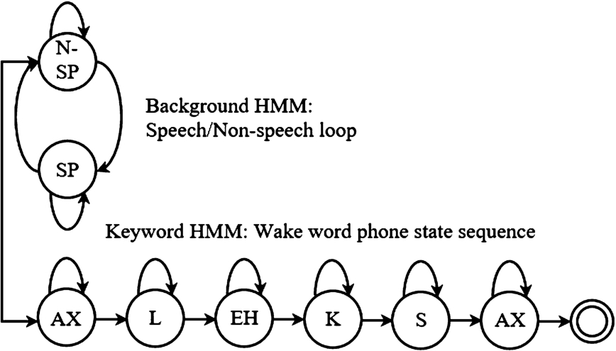
Each state of the model represents an acoustic unit (see Section 5 for details), for example, a phoneme. Model “says” that at each frame (see Section 3) the acoustic environment is in one of the states of the HMM and generates a visible variable, for example, the vector of the MFCC-features (or more generally, sound). Each state has a distribution of probabilities over the sound. Thus, when we receive an audio file, we know the sound and the probability distributions, but we do not know in what state the model was in each of the frames. However, for each possible sequence of states, we can calculate the probability of this sequence. By decoding (Section 6), we can find the most probable sequence. If this sequence generated a keyword, then we can say that the activation occurred (there are other options for decoding and determining the activation).

Fig. 2.

Hidden Markov model example for Amazon’s keyword spotter (Guo et al., 2018).

It is necessary to be able to calculate

P (S | s)

$ P(S|s)$

(s is an HMM state) to find the keyword. Such calculation is called acoustic modelling. Gaussian mixture model (GMM) or neural networks are the most frequent choices for acoustic model. Note that these choices coincide with the choices for acoustic models in automatic speech recognition systems. Before (Hinton et al., 2012) GMM acoustic models were considered state-of-the-art, and after the publication they were almost completely replaced by neural networks.

Note that it is the question of definitions what to consider an acoustic model in the HMM-GMM setup. You can either consider GMM (so the part which actually computes

P (S | s)

$ P(S|s)$

, recall that the HMM state often represents some acoustic unit) or the whole HMM, because it expresses

P (S | w)

$ P(S|w)$

like in Zheng et al. (1999) (w is a keyword).

Good acoustic model is the key for a high quality voice activation system. Therefore, it is not surprising that the calculations associated with the acoustic model usually take the biggest part of the voice activation system runtime. This is why in many studies this part is speeded up. For example, Fernández-Marqués et al. (2018) apply the binary arithmetic (instead of floating arithmetic) in the model, Sun et al. (2017), Szöke et al. (2010) represent the architecture of a neural network where each layer of the matrix multiplication of

N \times M

$ N\times M$

is replaced by the product of two matrices with sizes

N \times K

$ N\times K$

and

K \times M

$ K\times M$

, where K is much smaller than N and M. Thus, a big number of operations is saved, and not a lot of expressive power of the model is lost (with the appropriate method of training).

Another way to build a speech recognition system is not to use HMM, but to calculate some (heuristically selected) value based on the outputs of the acoustic model. For a successful use of this approach, see Chen et al. (2014a).

The acoustic models used in studied sources are presented in Table 8, in Appendix A. The number of times these models were used in the sources is presented in Table 2.

Table 2

The number of times a specific acoustic model was used in studied sources.

Acoustic model	Number of sources
GMM	18
Neural network	10
Time-delayed neural network	4
RNN, gated RNN, LSTM, bidirectional LSTM	2
Polynomial model, continous density neural tree, mixture of central distance normal distributions, support vector machine, deep neural network with highway blocks, binary deep neural network, convolutional neural network	1

5 Acoustic Units

The choice of an elementary unit for acoustic modelling (acoustic unit) affects the resulting quality. A system developer is faced with the following tradeoff: the larger the unit is (e.g. a word), the more stable it is (meaning, that produced acoustic features have less variability) and accordingly, it is easier to find such a pattern in audio stream. However, such a system is not flexible.

If a smaller unit has been chosen, for example, phoneme, then we are faced with a more difficult task of finding a pattern, but on the other hand we can build a system that finds an arbitrary word from a system that finds phonemes.

Sometimes the solution for this tradeoff is to choose syllables or part of the words if it is difficult to define syllables.

Also, one can choose not a whole phoneme as a unit, but a part of the phoneme (for example, the beginning of the phoneme A or the middle of the phoneme B) or context-dependent phoneme (for example, phoneme A, going after phoneme B). A phoneme without context is often called monophone, and a context-dependent is called biphone (if the dependency is only on one side) or triphone (if the dependency is on both the left and the right). There is also a possibility to combine these approaches and use part of the context-dependent phoneme. In this case, the system will probably have impractically many units, so they are often clustered (by pronunciation) into clusters called senones.

We must note that the term senone does not have a strict definition. Some authors like Yu and Deng (2014) define senone as a tied (clustered) triphone state. Some, like authors of Janus Toolkit, call all acoustic units senones (Janus Toolkit Documentation, 2019).

The solution of this tradeoff depends on the size of the training data (at a small size it is much more difficult to build a whole word model than a phoneme model), the choice of the acoustic model, the key phrase, and the language. As far as we know, at the moment there is no algorithm or rules, under what conditions which acoustic unit to choose.

The acoustic units used in studied sources are presented in Table 6 in Appendix A. Number of times these units were used in the sources are presented in Table 3.

Table 3
Number of times specific acoustic unit was used in studied sources.

Acoustic unit Number of sources

Monophone 19

Whole word 13

Syllable 5

Letter, part of the word, part of the phoneme 3

Triphone 2

State unit (learnt “phoneme”), senone 1

Acoustic unit	Number of sources
Monophone	19
Whole word	13
Syllable	5
Letter, part of the word, part of the phoneme	3
Triphone	2
State unit (learnt “phoneme”), senone	1

6 Decoding

As a result of the acoustic model application to an audio stream we receive the values characterizing probability that at a certain moment this or that acoustic unit was pronounced. Voice activation system needs to make a decision whether the keyword was uttered in an audio stream or not according to the obtained one or more numeric series. To do this, different approaches of decoding are used.

In the simplest case, it is only necessary to compare the obtained number with the threshold value to make a decision. E.g. when the acoustic unit is the whole keyword the decision is made by comparing the computed probability with 0.5.

Smoothing is usually used to improve the recognition quality in the case of comparison with the threshold (Chen et al., 2014a; Lehtonen, 2005). The motivation for this technique is that the keyword is an acoustic event that has a certain duration in the time dimension. Thus, the actual keyword utterance should generate a high probability of multiple counts in a row. Thus, when applying the smoothing function to the time series, we avoid false positives caused by fluctuations of the acoustic model. Silaghi and Vargiya (2005) suggested an interesting variant of smoothing. In the case of acoustic units, the probabilities of each phoneme are normalized to the probability of the least probable phoneme.

In systems that use a comparison with a template utterance, Dynamic Time Warping (DTW) is often used. DTW is an analogue of the Levenshtein distance for numerical series. The motivation of this method is that the duration of the recorded pattern is likely to differ from the pronunciation in real conditions. Thus, we cannot compare two audio fragment directly, namely, one needs “to strech” or “to squeeze” certain intervals of the template over time. DTW distance is usually computed with dynamic programming. For a more detailed description and various modifications, please refer to Zehetner et al. (2014).

Decoding becomes more meaningful in the case of HMM. Indeed, in this formulation, we need to solve a typical problem for HMM: find the most probable sequence of hidden states (if this sequence corresponds to a keyphrase, then, in some approaches, it means activation) or find the total probability of passing through some sequences of states (for example, we can say that we do not care how many frames in a row the first phrase phoneme was pronounced, how many, the second and so on; only the order is important).

The Viterby algorithm uses dynamic programming to find the most likely sequence of hidden states in hidden Markov model given the observations. Naturally, this algorithm is widely used in works about HMM-voice activation systems. Many authors explore a variety of approaches and heuristics to speed up the algorithm, adapt it to find sequences satisfying some additional properties, and so on. For example, Liu et al. (2000) use various techniques of hypotheses pruning and rescoring probabilities using a bi-gram language model. In Zhu et al. (2013), the possibility of using the Viterbi algorithm on sliding windows of the audio stream is considered. Junkawitsch et al. (1997) consider a modification of the Viterbi algorithm that approximates finding the optimal sequence that has the highest probability normalized by the utterance length. Several additional modifications of the Viterbi algorithm are considered in Wilcox and Bush (1992).

In addition, Wilcox and Bush (1992) discuss how to use the forward–backward algorithm for quick estimation of probabilities needed in decoding.

We would also like to mention the standard technique of using HMM-derived probabalities and deriving decoding to comparing to the threshold. This approach is conventionally called likelihood ratio. Often, two HMM are used: the speech model representing all the keyword pronunciations, and the garbage model representing all other audio events. In such systems, one can find the probability of passing through the garbage model and the probability of passing through the part with the keyword. Then the ratio of these two probabilities shows confidence in the presence of a key phrase in the audio stream. This ratio is compared with the threshold in many voice activation systems. It is worth noting that finding the balance of coefficients in such models is a difficult task, which is usually solved by optimizing the parameters on the held-out data set.

Some authors use completely different approaches to decode. For example, Manor and Greenberg (2017) describe an application of fuzzy logic to decoding.

The approaches to decode used in studied sources are presented in Table 9 in Appendix A. The numbers of times the specific approach was used in studied sources are presented in Table 4.

Table 4
Number of times the specific approach to decoding was used in studied sources.

Decoding approach Number of sources

Viterby 15

Comparing to threshold 11

DTW 5

Forward–Backward algorithm, likelihood ratio 2

Fuzzy logic 1

Decoding approach	Number of sources
Viterby	15
Comparing to threshold	11
DTW	5
Forward–Backward algorithm, likelihood ratio	2
Fuzzy logic	1

7 Quality Assessment

A large number of metrics can be used to compare different approaches of voice activation systems. These metrics can be grouped by the aspect of the system they measure:

•
classification quality,
•
operation speed,
•
amount of used RAM and CPU.

Metrics for speed measurement are standard and non-specific for voice activation systems. The most commonly used are real time factor (RTF) – total processing time of the audio stream divided by the length of the stream, latency (average delay of the response signal from pronouncing) and total processing time (this metric is less indicative than RTF).

For resource usage, it is the most popular to measure the amount of RAM used and CPU load (as a percentage of the compute core). To improve both parameters, different approaches to quantize the parameters of the acoustic model are often used (Fernández-Marqués et al., 2018).

But at the moment there are no standard metrics to measure the quality of classification. Moreover, similar metrics, unfortunately, are called differently in different sources. We think it would be profitable to have standartized set of metrics in that area.

The main problem is that the voice activation system must satisfy two opposite properties to work well: it must be sensitive enough to react to the keyword utterances, and it must be robust enough not to react to sound events similar to the keywords, but that are not actual keywords. Any system can be made arbitrarily sensitive, reacting to each event, and arbitrarily robust, not reacting to any events. The challenge is to choose the right balance between these two operating points. Therefore, one must either use at least two metrics (for example, precision and recall), or use one common metric (for example, f1-score) to measure the quality of a classification,. In the second case, an unsuccessful choice of metrics can lead to false conclusions, since there is no single correct balance between the importance of sensitivity and robustness.

The following metrics are often used to measure classification quality:
•
detection rate (precision) is the number of correctly recognized keywords relative to the total number of accepted keywords,
•
substitution rate is the number of mis-recognized keywrods relative to the total number of accepted keywords,
•
deletion rate (false reject rate, opposite to recall, miss rate) is the number of un-detected keywords relative to the total number of keywords,
•
rejection rate is the number of keywords which are rejected relative to the total number of keywords (false reject rate – FRR),
•
false alarm rate (FAR) is the number of false alarms (relative to the number of utterances without keyword; sometimes per keyword or per hour of speech),
•
accuracy (recognition rate) is the number of correctly classified utterances relative to the total number of utterances,
•
true positive rate (same as recall),
•
true negative rate (opposite to FAR).

As you can see, there is no accepted pair of metrics, moreover, often the same metrics are not called the same in different sources.

Figure of merit is one of the most used metrics in voice activation system research. FOM is the average of correct detections per k false positive activations per hour for each natural number k from 1 to 10. This metric was especially often used until the 2010s. Recently, such high rates of false positives per hour are unreasonably high, so FOM does not reflect the relevant modes of operation of the modern voice activation system. Other common metrics are equal error rate (the smallest value that can take both FAR and FRR at the same time), ROC-AUC (the area under the precision-recall curve).

Some papers suggest more complex ways of measuring classification quality. For example, disriminative error rate is introduced in Cuayáhuitl and Serridge (2002). In this metric different errors (when the system asked the user for confirmation, or rejected the operation without confirmation) have different penalties. In our opinion, this approach is more suitable for quality assesment for real product use of systems.

It is hard to compare results from different works not only because different metrics are used, but also because the choice of the dataset and the keyword deeply affects the results. If two works use false alarms per hour to describe their system quality, but one uses a dataset of speech recordings and the other uses a dataset from real user devices (where speech may take 3–6 hours for each 24 hour recording), then these works would have completely different metrics even with the same voice activation system.

We think it is safe to assume that industry research provides the best or close to the best voice activation systems today because of big amount of audio data and computation resources. Shan et al. (2018) reports system with
$1.02 %$ $ 1.02\% $
FRR with 1 false alarm per hour. This model has 84,000 parameters. Raziel and Hyun-Jin (2018) claims that their “Ok Google” voice activation systems has FRR from
$0.87 %$ $ 0.87\% $
(clean non-accented utterances) to
$8.90 %$ $ 8.90\% $
(real user query logs) with 0.1 false alarm per hour with 700,000 parameters. Fernández-Marqués et al. (2018) tell that it’s possible to create a competitive voice activation system that would use 15.8 kB of memory and would perform 2 million operations per inference pass.

The metrics used in studied sources are presented in Table 10 in Appendix A. The numbers of times these metrics were used in studied sources are presented in Table 5.

Table 5
Number of times the specific metric was used in studied sources.

Metrics Number of sources

FOM 20

False alarm rate 12

ROC 8

False reject rate, accuracy 6

False alarm per kw per hour 5

Detection rate, recall 4

Custom, recognition rate, real time factor 3

Equal error rate, deletion rate, rejection rate, precision 2

Insertion rate, discriminative error rate, substitution rate, true positive rate, false positive rate, miss rate, F1, latency, mean time between false alarms, processing time, misses, hits, RAM usage, flops, accuracy to size, accuracy to ops 1

8 Unconventional Approaches

Metrics	Number of sources
FOM	20
False alarm rate	12
ROC	8
False reject rate, accuracy	6
False alarm per kw per hour	5
Detection rate, recall	4
Custom, recognition rate, real time factor	3
Equal error rate, deletion rate, rejection rate, precision	2
Insertion rate, discriminative error rate, substitution rate, true positive rate, false positive rate, miss rate, F1, latency, mean time between false alarms, processing time, misses, hits, RAM usage, flops, accuracy to size, accuracy to ops	1

Some approaches to the construction of voice activation systems are difficult to describe according to the classification proposed in Section 2.

First of all it worth to mention approaches of comparison with a template, for example using DTW. In such systems, the user first records one or several keywords pronunciations, and then the necessary sound fragments are compared with the recordings and the triggering is announced if the selected similarity measure exceeds some prespecified threshold. The advantages of this approach include the simplicity of both learning (memorization) and operation. In addition, in this approach, it is natural to use personalization: indeed, one can argue that recorded patterns reflect the specific features of the user pronunciation, which allow to distinguish it from other users if appropriate similarity metric is used. However, in practice this approach is not very robust. The quality of its operation depends on how well the similarity measure is chosen and what features are used. The task to eliminate all the noise and disimilarity in environments by appropriate choice of features and similarity measure has proven to be difficult. DTW is one way to calculate the measure of similarity of two time series, possibly of different length. Systems using such approaches are described in Morgan et al. (1991), Naylor et al. (1992), Zeppenfeld and Waibel (1992), Kosonocky and Mammone (1995), Kurniawati et al. (2012). Zehetner et al. (2014) discuss the different underlying metrics of the similarity to use in DTW framework. Szöke et al. (2015) discuss the possibility of using DTW even for the case where a keyword can be subjected to declensions, conjugations, or even word order permutations.

Another interesting approach is to model the appearance (or absence) of keywords with the help of point processes and, in particular, Poisson processes. In such systems, the parameters of two process families are evaluated: for each selected feature for sound with (1) and without a keyword (2). An interesting feature of such systems is the ability to select these parameters during operation, thereby adapting to the channel, user and usage scenarios. For more information on the proposed see Jansen and Niyogi (2009c), Jansen and Niyogi (2009b). Sadhu and Ghosh (2017) describe how to apply this approach in systems with limited resources using unsupervised online learning.

Finally we would like to mention the discriminative keyword spotting, an approach that was introduced in Keshet et al. (2009). In this approach, instead of using an HMM or a similar model, the audio track is embedded in the feature space. Then, a linear (or more complex) model in this space is trained to distinguish positive (with a keyword) and negative (without a keyword) examples. This allows the use of support vector machine-like (SVM) approaches to maximize the margin from separating hyperplane. In addition, the task of training in such a system can be set as the task of maximizing the area under the ROC-curve, which is one of the common metrics for assessing the quality of the voice activation system. In such systems, it is necessary to use feature engineering, which can be both a advantage (one can easily embed prior knowledge) and a disadvantage (incorrect prior knowledge leads to poor quality of work; in addition, feature engineering is a complex manual process). In subsequent works, this approach is developed. Wöllmer et al. (2009b) add a hidden layer of bidirectional LSTM network as features, Tabibian et al. (2011) use a genetic algorithm instead of a linear classifier, and Tabibian et al. (2014) describe the use of kernel trick within the framework of discriminative keyword spotting. A very detailed explanation of disriminative keyword spotting can also be found in Tabibian et al. (2013; 2016).

9 Conclusion

In this research, we have made a systematic literature review of voice activation systems. We proposed the structure of a typical voice activation system and considered main approaches described in the literature for each of the modules of such a system.

Regarding the feature representation, most of the techniques are shared with automatic speech recognition. The majority of cited works use MFCC or Log Mel-filterbank features. In this area, we see the reduction of the inductive bias over the time: more and more recent papers like (Raziel and Hyun-Jin, 2018) or (Myer and Tomar, 2018) don not use DCT-step, probably because deep neural networks work reasonably well even with correlated features. We expect further simplification: using raw waveform or some unsupervised approach like contrastive predictive coding in Oord et al. (2018).

GMM, widely used in acoustic modelling, are replaced with different types of neural networks. We are not aware of any state-of-the-art solutions that do not use deep learning in the voice activation problem. One of the main questions in that area is how to apply neural networks having limited resources. Some possible answers are: to apply quantization, to use a special network topology like time-delayed neural network or to use a cascade of the models waking up the more powerful and consuming model only if the smaller model is activated.

At the moment, the most widely used systems use phonemes as acoustic units. Phonemes are stable enough to be reliably found in audio stream and flexible enough to be used for the majority (if not all) keywords.

We believe that voice activation research could greatly benefit from creating open datasets in order to compare different systems. Today it is complicated to compare different works because of different train and test data, different keywords, and sometimes different target metrics.

As a result of the literature review, we noticed that there are some questions to which there are no clear answers in the published sources. So we would like to focus on them and conduct research in these areas:

•
Are there common acoustic features suitable for all languages? How do we understand what features does it need for a given language? Indeed, most of the works are building voice activation systems for the English language, for which the MFCC and Log Mel-filterbank have proven themselves well. Researchers who used systems for other languages faced the necessity to use other features (Ida and Yamasaki, 1998; Zheng et al., 1999).
•
Does the quality of activation depend on which acoustic unit is used for the language? A similar question was investigated for Spanish in Cuayáhuitl and Serridge (2002) and for Chinese in Liu et al. (2000), but the problem of determining the most appropriate acoustic unit for an arbitrary language was not investigated.
•
Are there any criteria on how to choose keywords to activate? This question is important both for the practical application of the voice activation system and for an objective comparison of systems with each other. We noticed that the acoustic features and the length of the keyword have a significant impact on the quality of activation. For example, in Jansen and Niyogi (2009a) it is shown that there is a strong correlation between the quality of work and the length of the keyword. However, an open question as to what other properties of the key phrase are important for the good operation of the system remains. Also it would be interesting to investigate whether are there any general rules for choosing a good keyword.

A Appendix

Table 6

Acoustic units used in studied sources.

Acoustic unit	Sources
Whole word	(Morgan et al., 1990; Rose and Paul, 1990; Morgan et al., 1991; Naylor et al., 1992; Rohlicek et al., 1993; Cuayáhuitl and Serridge, 2002; Baljekar et al., 2014; Chen et al., 2014a; Zehetner et al., 2014; Hou et al., 2016; Manor and Greenberg, 2017; Fernández-Marqués et al., 2018; Myer and Tomar, 2018)
Monophone	(Rose and Paul, 1990; Rohlicek et al., 1993; Cuayáhuitl and Serridge, 2002; Heracleous and Shimizu, 2003; Szöke et al., 2005; Lehtonen, 2005; Silaghi and Vargiya, 2005; Wöllmer et al., 2009b; Jansen and Niyogi, 2009a,c; Wöllmer et al., 2009a; Szöke et al., 2010; Shokri et al., 2011; Tabibian et al., 2011; Hou et al., 2016; Kumatani et al., 2017; Gruenstein et al., 2017; Tabibian et al., 2018; Myer and Tomar, 2018)
Triphone	(Rose and Paul, 1990; Szöke et al., 2005)
Part of the word	(Naylor et al., 1992; Li and Wang, 2014; Chen et al., 2014a)
State unit	(Zeppenfeld and Waibel, 1992)
Part of the phoneme	(Rohlicek et al., 1989; Kosonocky and Mammone, 1995; Leow et al., 2012)
Syllable	(Klemm et al., 1995; Zheng et al., 1999; Liu et al., 2000; Cuayáhuitl and Serridge, 2002; Hou et al., 2016)
Letter	(Hwang et al., 2015; Hou et al., 2016; Lengerich and Hannun, 2016)
Senone	(Ge and Yan, 2017)

Table 7

Acoustic features used in studied sources.

Acoustic features and transformations	Sources
MFCC	(Rose and Paul, 1990; Vroomen and Normandin, 1992; Junkawitsch et al., 1997; Liu et al., 2000; Heracleous and Shimizu, 2003; Khne et al., 2004; Szöke et al., 2005; Keshet et al., 2009; Wöllmer et al., 2009b; Bahi and Benati, 2009; Jansen and Niyogi, 2009c; Vasilache and Vasilache, 2009; Wöllmer et al., 2009a; Tabibian et al., 2011; Leow et al., 2012; Wöllmer et al., 2013; Shokri et al., 2013; Zhu et al., 2013; Baljekar et al., 2014; Sangeetha and Jothilakshmi, 2014; Shokri et al., 2014; Zehetner et al., 2014; Laszko, 2016; Manor and Greenberg, 2017; Fernández-Marqués et al., 2018)
Log Mel-filterbank	(Morgan et al., 1990, 1991; Zeppenfeld and Waibel, 1992; Chen et al., 2014a; Hwang et al., 2015; Hou et al., 2016; Gruenstein et al., 2017; Sun et al., 2017; Myer and Tomar, 2018)
Fourier transform	(Morgan et al., 1990, 1991; Zeppenfeld and Waibel, 1992; Guo et al., 2018)
LPC	(Gish et al., 1990, 1992; Gish and Ng, 1993; Rohlicek et al., 1993; Zheng et al., 1999; Rohlicek et al., 1989)
Derivatives or deltas	(Gish et al., 1990; Rose and Paul, 1990; Vroomen and Normandin, 1992; Gish and Ng, 1993; Junkawitsch et al., 1997; Liu et al., 2000; Heracleous and Shimizu, 2003; Khne et al., 2004; Szöke et al., 2005; Keshet et al., 2009; Wöllmer et al., 2009b; Jansen and Niyogi, 2009c; Vasilache and Vasilache, 2009; Wöllmer et al., 2009a; Tabibian et al., 2011; Leow et al., 2012; Wöllmer et al., 2013; Shokri et al., 2013; Baljekar et al., 2014; Chen et al., 2014a; Sangeetha and Jothilakshmi, 2014; Shokri et al., 2014; Hwang et al., 2015; Ge and Yan, 2017)
Energy or log-energy	(Vroomen and Normandin, 1992; Heracleous and Shimizu, 2003; Khne et al., 2004; Wöllmer et al., 2013; Hwang et al., 2015)
Mean/variance normalization	(Gish et al., 1992; Gish and Ng, 1993; Rohlicek et al., 1993; Jansen and Niyogi, 2009c; Wöllmer et al., 2009a; Shokri et al., 2011; Sangeetha and Jothilakshmi, 2014; Myer and Tomar, 2018)
Gain normalization	(Shokri et al., 2011)
Stacking	(Junkawitsch et al., 1997; Chen et al., 2014a; Fernández-Marqués et al., 2018)
LDA over MFCC	(Junkawitsch et al., 1997)
Prosodic information	(Ida and Yamasaki, 1998)
PCP	(Szöke et al., 2005; Chen et al., 2014a; Ge and Yan, 2017)
AMA	(Shokri et al., 2011)
Spectral entropy, spectral flatness, burst degree, bisector frequency	(Tabibian et al., 2011)
Formant frequencies	(Laszko, 2016)
f-MLLR	(Sadhu and Ghosh, 2017)
Raw waveform	(Kumatani et al., 2017)

Table 8

Acoustic models used in studied resources.

Acoustic model	Sources
NN	(Morgan et al., 1990; Szöke et al., 2005; Lehtonen, 2005; Szöke et al., 2010; Chen et al., 2014b; Hou et al., 2016; Gruenstein et al., 2017; Ge and Yan, 2017; Wu et al., 2018; Myer and Tomar, 2018)
GMM	(Rohlicek et al., 1989; Rose and Paul, 1990; Vroomen and Normandin, 1992; Junkawitsch et al., 1997; Liu et al., 2000; Heracleous and Shimizu, 2003; Khne et al., 2004; Szöke et al., 2005; Jansen and Niyogi, 2009a,c; Vasilache and Vasilache, 2009; Shokri et al., 2011; Leow et al., 2012; Zhu et al., 2013; Baljekar et al., 2014; Li and Wang, 2014; Chen et al., 2014a; Benisty et al., 2018)
RNN	(Naylor et al., 1992; Baljekar et al., 2014)
Gated RNN	(Baljekar et al., 2014; Hou et al., 2016)
TDNN	(Zeppenfeld and Waibel, 1992; Kumatani et al., 2017; Sun et al., 2017; Myer and Tomar, 2018)
Polynomial model	(Gish and Ng, 1993)
Continous density neural tree	(Kosonocky and Mammone, 1995)
Mixture of central distance normal distributions	(Zheng et al., 1999)
LSTM	(Hwang et al., 2015; Hou et al., 2016)
Bi-LSTM	(Wöllmer et al., 2009a; Zhang et al., 2016)
SVM	(Tabibian et al., 2011)
DNN with highway blocks	(Guo et al., 2018)
Binary DNN	(Fernández-Marqués et al., 2018)
CNN	(Myer and Tomar, 2018)

Table 9

The approaches to decoding used in studied sources.

Decoding approach	Sources
Comparing to threshold	(Morgan et al., 1990; Naylor et al., 1992; Junkawitsch et al., 1997; Keshet et al., 2009; Wöllmer et al., 2009b,a; Li and Wang, 2014; Chen et al., 2014a; Gruenstein et al., 2017; Benisty et al., 2018; Myer and Tomar, 2018)
Viterby	(Rose and Paul, 1990; Feng and Mazor, 1992; Wilcox and Bush, 1992; Rohlicek et al., 1993; Knill and Young, 1996; Junkawitsch et al., 1997; Zheng et al., 1999; Liu et al., 2000; Vasilache and Vasilache, 2009; Tabibian et al., 2011; Leow et al., 2012; Zhu et al., 2013; Kumatani et al., 2017; Ge and Yan, 2017; Sun et al., 2017)
Forward–Backward algorithm	(Wilcox and Bush, 1992; Rohlicek et al., 1993)
DTW	(Zeppenfeld and Waibel, 1992; Kosonocky and Mammone, 1995; Kurniawati et al., 2012; Zehetner et al., 2014; Hou et al., 2016)
Likelihood ratio	(Jansen and Niyogi, 2009c; Szöke et al., 2010)
Fuzzy logic	(Manor and Greenberg, 2017)

Table 10

The metrics used in studied sources.

Metrics	Sources
FOM	(Gish et al., 1990; Rose and Paul, 1990; Naylor et al., 1992; Zeppenfeld and Waibel, 1992; Chang and Lippmann, 1994; Gish and Ng, 1993; Rohlicek et al., 1993; Knill and Young, 1996; Junkawitsch et al., 1997; Zheng et al., 1999; Szöke et al., 2005; Lehtonen, 2005; Jansen and Niyogi, 2009a,c; Szöke et al., 2010; Tabibian et al., 2011; Bohac, 2012; Sangeetha and Jothilakshmi, 2014; Sadhu and Ghosh, 2017; Tabibian et al., 2018)
EER	(Szöke et al., 2010; Bohac, 2012)
Accuracy	(Morgan et al., 1990, 1991; Ida and Yamasaki, 1998; Ge and Yan, 2017; Benisty et al., 2018; Fernández-Marqués et al., 2018)
FA/kw/h	(Rohlicek et al., 1989; Vroomen and Normandin, 1992; Feng and Mazor, 1992; Leow et al., 2012; Kavya and Karjigi, 2014)
ROC	(Marcus, 1992; Siu et al., 1994; Keshet et al., 2009; Wöllmer et al., 2009b, 2013; Shokri et al., 2013; Sadhu and Ghosh, 2017; Kumatani et al., 2017)
Detection rate	(Feng and Mazor, 1992; Khne et al., 2004; Shokri et al., 2011; Leow et al., 2012)
Substitution rate	(Feng and Mazor, 1992)
Deletion rate	(Feng and Mazor, 1992; Kavya and Karjigi, 2014)
Rejection rate	(Feng and Mazor, 1992; Heracleous and Shimizu, 2003)
Insertion rate	(Klemm et al., 1995)
Recognition rate	(Liu et al., 2000; Heracleous and Shimizu, 2003; Zhu et al., 2013)
Discriminative error rate	(Cuayáhuitl and Serridge, 2002)
FAR	(Khne et al., 2004; Shokri et al., 2011; Chen et al., 2014a; Hou et al., 2016; Gruenstein et al., 2017; Ge and Yan, 2017; Sun et al., 2017; Tabibian et al., 2018; Benisty et al., 2018; Guo et al., 2018; Wu et al., 2018; Myer and Tomar, 2018)
FRR	(Chen et al., 2014a; Gruenstein et al., 2017; Sun et al., 2017; Guo et al., 2018; Wu et al., 2018; Myer and Tomar, 2018)
RTF	(Szöke et al., 2005; Bohac, 2012; Tabibian et al., 2018)
TPR, FPR	(Wöllmer et al., 2009a)
Miss rate	(Hou et al., 2016)
Recall	(Baljekar et al., 2014; Li and Wang, 2014; Zehetner et al., 2014; Hwang et al., 2015)
Precision	(Zehetner et al., 2014; Hwang et al., 2015)
F1, latency	(Hwang et al., 2015)
Mean time between false alarms	(Baljekar et al., 2014)
Processing time	(Li and Wang, 2014)
Misses, hits	(Li and Wang, 2014)
RAM usage, flops, accuracy to size, accuracy to ops	(Fernández-Marqués et al., 2018)
Custom	(Marcus, 1992; Silaghi and Vargiya, 2005; Szöke et al., 2010)

References

Bahi

Benati

(2009). A new keyword spotting approach. In: 2009 International Conference on Multimedia Computing and Systems, pp. 77–80.

Baljekar

Lehman

J.F.

Singh

(2014). Online word-spotting in continuous speech with recurrent neural networks. In: 2014 IEEE Spoken Language Technology Workshop, SLT 2014, South Lake Tahoe, NV, USA, December 7–10, 2014, pp. 536–541.

Benisty

Katz

Crammer

Malah

(2018). Discriminative keyword spotting for limited-data applications. Speech Communication, 99, 1–11.

Bohac

(2012). Performance comparison of several techniques to detect keywords in audio streams and audio scene. In: Proceedings ELMAR-2012, pp. 215–218.

Chang

E.I.

Lippmann

R.P.

(1994). Figure of merit training for detection and spotting. In: Cowan

J.D.

Tesauro

Alspector

(Eds.), Advances in Neural Information Processing Systems, Vol. 6. Morgan-Kaufmann, pp. 1019–1026.

Chen

Parada

Heigold

(2014a). Small-footprint keyword spotting using deep neural networks. 4-9, 2014. IEEE. In: IEEE International Conference on Acoustics, Speech and Signal Processing, ICASSP 2014, Florence, Italy, May 4–9, 2014. IEEE, pp. 4087–4091.

Chen

N.F.

Sivadas

Lim

B.P.

Ngo

H.G.

Pham

V.T.

(2014b). Strategies for Vietnamese keyword search. In: IEEE International Conference on Acoustics, Speech and Signal Processing, ICASSP 2014, Florence, Italy, May, May 4–9, 2014. IEEE, pp. 4121–4125.

Cuayáhuitl

Serridge

(2002). Out-of-vocabulary word modeling and rejection for Spanish keyword spotting systems. In: Coello

C.A.C.

deAlbornoz

Sucar

L.E.

Battistutti

O.C.

(Eds.), MICAI 2002: Advances in Artificial Intelligence, Second Mexican International Conference on Artificial Intelligence, Merida, Yucatan, Mexico, April 22–26, 2002, Proceedings, Lecture Notes in Computer Science , Vol. 2313. Springer, pp. 156–165.

Feng

Mazor

(1992). Continuous word spotting for applications in telecommunications. In: The Second International Conference on Spoken Language Processing, ICSLP 1992, Banff, Alberta, Canada, October 13–16, 1992, ISCA.

10.

Fernández-Marqués

Tseng

V.W.S.

Bhattacharya

Lane

N.D.

(2018). Deterministic binary filters for keyword spotting applications. In: Ott

Dressler

Saroiu

Dutta

(Eds.), Proceedings of the 16th Annual International Conference on Mobile Systems, Applications, and Services, MobiSys 2018, Munich, Germany, June 10–15, 2018. ACM, p. 529.

11.

Yan

(2017). Deep neural network based wake-up-word speech recognition with two-stage detection. 5-9, 2017. IEEE. In: 2017 IEEE International Conference on Acoustics, Speech and Signal Processing, ICASSP 2017, New Orleans, LA, USA, March 5–9, 2017. IEEE, pp. 2761–2765.

12.

Giannakopoulos

(2015). epyAudioAnalysis: an open-source Python library for audio signal analysis. PloS One, 10(12).

13.

Gish

(1993). A segmental speech model with applications to word spotting. In: 1993 IEEE International Conference on Acoustics, Speech, and Signal Processing, Vol. 2, pp. 447–450.

14.

Gish

Chow

Y.L.

Rohlicek

J.R.

(1990). Probabilistic vector mapping of noisy speech parameters for HMM word spotting. In: International Conference on Acoustics, Speech, and Signal Processing, Vol. 1, pp. 117–120.

15.

Gish

Rohlicek

J.R.

(1992). Secondary processing using speech segments for an HMM word spotting system. In: The Second International Conference on Spoken Language Processing, ICSLP 1992, Banff, Alberta, Canada, October 13–16, 1992, ISCA.

16.

Gruenstein

Alvarez

Thornton

Ghodrat

(2017). A cascade architecture for keyword spotting on mobile devices. CoRR, abs/1712.03603.

17.

Guo

Kumatani

Sun

Raju

Strom

Mandal

(2018). Time-delayed bottleneck highway networks using a DFT feature for keyword spotting. In: 2018 IEEE International Conference on Acoustics, Speech and Signal Processing, ICASSP 2018, Calgary, AB, Canada, April 15–20, 2018. IEEE, pp. 5489–5493.

18.

Hao

(2002). Word spotting based ona posterior measure of keyword confidence. Journal of Computer Science and Technology, 17(4), 491–497.

19.

Heracleous

Shimizu

(2003). An efficient keyword spotting technique using a complementary language for filler models training. In: 8th European Conference on Speech Communication and Technology, EUROSPEECH 2003 – INTERSPEECH 2003, Geneva, Switzerland, September 1–4, 2003, ISCA.

20.

Hinton

Deng

Dahl

Mohamed

A.R.

Jaitly

Senior

Vanhoucke

Nguyen

Kingsbury

Sainath

(2012). Deep neural networks for acoustic modeling in speech recognition. IEEE Signal Processing Magazine, 29, 82–97.

21.

Hou

Xie

(2016). Investigating neural network based query-by-example keyword spotting approach for personalized wake-up word detection in Mandarin Chinese. In: 10th International Symposium on Chinese Spoken Language Processing, ISCSLP 2016, Tianjin, China, October 17–20, 2016. IEEE. pp. 1–5.

22.

Hwang

Lee

Sung

(2015). Online keyword spotting with a character-level recurrent neural network. CoRR. abs/1512.08903.

23.

Ida

Yamasaki

(1998). An evaluation of keyword spotting performance utilizing false alarm rejection based on prosodic information. In: The 5th International Conference on Spoken Language Processing, Incorporating The 7th Australian International Speech Science and Technology Conference, Sydney Convention Centre, Sydney, Australia, 30th November–4th December 1998, ISCA.

24.

Jansen

Niyogi

(2009a). An experimental evaluation of keyword-filler hidden markov models. Tech. Rep., Department of Computer Science, University of Chicago.

25.

Jansen

Niyogi

(2009b). Point process models for spotting keywords in continuous speech. Transactions on Audio, Speech, and Language Processing, 17(8), 1457–1470.

26.

Jansen

Niyogi

(2009c). Robust keyword spotting with rapidly adapting point process models. In: INTERSPEECH 2009, 10th Annual Conference of the International Speech Communication Association, Brighton, United Kingdom, September 6–10, 2009. ISCA, pp. 2767–2770.

27.

Janus Toolkit Documentation (2019). http://www.cs.cmu.edu/∼tanja/Lectures/JRTkDoc/OldDoc/senones/sn_main.html, Accessed 30th June 2019.

28.

Junkawitsch

Ruske

Höge

(1997). Efficient methods for detecting keywords in continuous speech. In: Kokkinakis

Fakotakis

Dermatas

(Eds.), Fifth European Conference on Speech Communication and Technology, EUROSPEECH 1997, Rhodes, Greece, September 22–25, 1997, ISCA.

29.

Kavya

H.P.

Karjigi

(2014). Sensitive keyword spotting for crime analysis. In: 2014 IEEE National Conference on Communication, Signal Processing and Networking (NCCSN), pp. 1–6.

30.

Keshet

Grangier

Bengio

(2009). Discriminative keyword spotting. Speech Communication, 51(4), 317–329.

31.

Këpuska

Klein

(2009). A novel Wake-Up-Word speech recognition system, Wake-Up-Word recognition task, technology and evaluation. Nonlinear Analysis: Theory, Methods & Applications, e2772(12), 45–e2789.

32.

Khne

Wolff

Eichner

Hoffmann

(2004). Voice activation using prosodic features. In: INTERSPEECH 2004 – ICSLP, 8th International Conference on Spoken Language Processing, Jeju Island, Korea, October 4–8, 2004, ISCA.

33.

Klemm

Class

Kilian

(1995). Word- and phrase spotting with syllable-based garbage modelling. In: Fourth European Conference on Speech Communication and Technology, EUROSPEECH 1995, Madrid, Spain, September 18–21, 1995, ISCA.

34.

Knill

K.M.

Young

S.J.

(1996). Fast implementation methods for Viterbi-based word-spotting. In: 1996 IEEE International Conference on Acoustics, Speech, and Signal Processing Conference Proceedings, Vol. 1, pp. 522–525.

35.

Kosonocky

S.V.

Mammone

R.J.

(1995). A continuous density neural tree network word spotting system. In: 1995 International Conference on Acoustics, Speech, and Signal Processing, Vol. 1, pp. 305–308.

36.

Kumatani

Panchapagesan

Kim

Strom

Tiwari

Mandal

(2017). Direct modeling of raw audio with DNNS for wake word detection. In: 2017 IEEE Automatic Speech Recognition and Understanding Workshop, ASRU 2017, Okinawa, Japan, December 16–20, 2017. IEEE, pp. 252–257.

37.

Kurniawati

Celetto

Capovilla

George

(2012). Personalized voice command systems in multi modal user interface. In: 2012 IEEE International Conference on Emerging Signal Processing Applications, ESPA 2012, Las Vegas, NV, USA, January 12–14, 2012. IEEE, pp. 45–47.

38.

Laszko

(2016). Using formant frequencies to word detection in recorded speech. In: Ganzha

Maciaszek

L.A.

Paprzycki

(Eds.), Proceedings of the 2016 Federated Conference on Computer Science and Information Systems, FedCSIS 2016, Gdańsk, Poland, September 11–14, 2016, pp. 797–801.

39.

Lehtonen

(2005). Hierarchical approach for spotting keywords. Idiap-RR Idiap-RR-41-2005, IDIAP.

40.

Lengerich

C.T.

Hannun

A.Y.

(2016). An End-to-End Architecture for Keyword Spotting and Voice Activity Detection. CoRR. abs/1611.09405.

41.

Leow

S.J.

Lau

T.S.

Goh

Peh

H.M.

T.K.

Siniscalchi

S.M.

Lee

(2012). A new confidence measure combining hidden Markov models and artificial neural networks of phonemes for effective keyword spotting. In: 8th International Symposium on Chinese Spoken Language Processing, ISCSLP 2012. Kowloon Tong, China, December 5–8, 2012. IEEE, pp. 112–116.

42.

Wang

(2014). A novel coding scheme for keyword spotting. In: 2014 Seventh International Symposium on Computational Intelligence and Design, Vol. 2, pp. 379–382.

43.

Liu

Chiu

Chang

(2000). Design of vocabulary-independent Mandarin keyword spotters. IEEE Trans. Speech and Audio Processing, 8(4), 483–487.

44.

Manor

Greenberg

(2017). Voice trigger system using fuzzy logic. In: 2017 International Conference on Circuits, System and Simulation (ICCSS), pp. 113–118.

45.

Marcus

J.N.

(1992). A novel algorithm for HMM word spotting performance evaluation and error analysis. In: [Proceedings] ICASSP-92: 1992 IEEE International Conference on Acoustics, Speech, and Signal Processing, Vol. 2, pp. 89–92.

46.

Morgan

D.P.

Scofield

C.L.

(1991). Neural Networks and Speech Processing. Springer US, Boston, MA, pp. 329–348.

47.

Morgan

D.P.

Scofield

C.L.

Lorenzo

T.M.

Real

E.C.

Loconto

D.P.

(1990). A keyword spotter which incorporates neural networks for secondary processing. In: International Conference on Acoustics, Speech, and Signal Processing, Vol. 1, pp. 113–116.

48.

Morgan

D.P.

Scofield

C.L.

Adcock

J.E.

(1991). Multiple neural network topologies applied to keyword spotting. In: [Proceedings] ICASSP 91: 1991 International Conference on Acoustics, Speech, and Signal Processing, Vol. 1, pp. 313–316.

49.

Myer

Tomar

V.S.

(2018). Efficient keyword spotting using time delay neural networks. In: Yegnanarayana

(Ed.), Interspeech 2018, 19th Annual Conference of the International Speech Communication Association, Hyderabad, India, 2–6 September 2018. ISCA, pp. 1264–1268.

50.

Naylor

J.A.

Huang

W.Y.

Nguyen

K.P.

(1992). The application of neural networks to wordspotting. In: 1992 Conference Record of the Twenty-Sixth Asilomar Conference on Signals, Systems Computers, Vol. 2, pp. 1081–1085.

51.

Oord

Vinyals

(2018). Representation Learning with Contrastive Predictive Coding.

52.

Povey

Ghoshal

Boulianne

Burget

Glembek

Goel

Hannemann

Motlicek

Qian

Schwarz

Silovsky

Stemmer

Vesely

(2011). The Kaldi speech recognition toolkit. In: IEEE 2011 Workshop on Automatic Speech Recognition and Understanding. IEEE Signal Processing Society, iEEE Catalog No.: CFP11SRW-USB.

53.

Raziel

Hyun-Jin

(2018). End-to-End Streaming Keyword Spotting.

54.

Rohlicek

J.R.

Russell

Roukos

Gish

(1989). Continuous hidden Markov modeling for speaker-independent word spotting. In: International Conference on Acoustics, Speech, and Signal Processing, Vol. 1, pp. 627–630.

55.

Rohlicek

J.R.

Jeanrenaud

Gish

Musicus

Siu

(1993). Phonetic training and language modeling for word spotting. In: 1993 IEEE International Conference on Acoustics, Speech, and Signal Processing, Vol. 2, pp. 459–462.

56.

Rose

R.C.

Paul

D.B.

(1990). A hidden Markov model based keyword recognition system. In: International Conference on Acoustics, Speech, and Signal Processing, Vol. 1, pp. 129–132.

57.

Sadhu

Ghosh

P.K.

(2017). Low resource point process models for keyword spotting using unsupervised online learning. In: 25th European Signal Processing Conference, EUSIPCO 2017, Kos, Greece, August 28–September 2, 2017. IEEE, pp. 538–542.

58.

Sangeetha

Jothilakshmi

(2014). A novel spoken keyword spotting system using support vector machine. Engineering Applications of Artificial Intelligence, 36, 287–293.

59.

Shan

Zhang

Wang

Xie

(2018). Attention-based end-to-end models for small-footprint keyword spotting. In: Proc. Interspeech 2018, pp. 2037–2041. https://doi.org/10.21437/Interspeech.2018-1777.

60.

Shokri

Tabibian

Akbari

Nasersharif

Kabudian

(2011). A robust keyword spotting system for Persian conversational telephone speech using feature and score normalization and ARMA filter. In: 2011 IEEE GCC Conference and Exhibition (GCC), pp. 497–500.

61.

Shokri

Davarpour

M.H.

Akbari

Nasersharif

(2013). Detecting keywords in Persian conversational telephony speech using a discriminative English keyword spotter. In: IEEE International Symposium on Signal Processing and Information Technology, Athens, Greece, December 12–15, 2013. IEEE Computer Society, pp. 272–276.

62.

Shokri

Davarpour

M.H.

Akbari

(2014). Improving keyword detection rate using a set of rules to merge HMM-based and SVM-based keyword spotting results. In: 2014 International Conference on Advances in Computing, Communications and Informatics, ICACCI 2014, Delhi, India, September 24–27, 2014, IEEE, pp. 1715–1718.

63.

Silaghi

Vargiya

(2005). A new evaluation criteria for keyword spotting techniques and a new algorithm. ISCA. In: INTERSPEECH 2005 - Eurospeech, 9th European Conference on Speech Communication and Technology, Lisbon, Portugal, September 4–8, 2005. ISCA, pp. 1593–1596.

64.

Siu

Gish

Rohlicek

J.R.

(1994). Predicting word spotting performance. In: The 3rd International Conference on Spoken Language Processing, ICSLP, 1994, Yokohama, Japan, September 18–22, 1994, ISCA.

65.

Sun

Snyder

Gao

Nagaraja

Rodehorst

Panchapagesan

Strom

Matsoukas

Vitaladevuni

(2017). Compressed time delay neural network for small-footprint keyword spotting. In: Lacerda

(Ed.), Interspeech 2017, 18th Annual Conference of the International Speech Communication Association, Stockholm, Sweden, August 20–24, 2017. ISCA, pp. 3607–3611.

66.

Szöke

Schwarz

Matejka

Burget

Karafiát

Cernocký

(2005). Phoneme based acoustics keyword spotting in informal continuous speech. In: Matousek

Mautner

Pavelka

(Eds.), Text, Speech and Dialogue, 8th International Conference, TSD 2005, Karlovy Vary, Czech Republic, September 12–15, 2005. Proceedings, Lecture Notes in Computer Science, Vol. 3658. Springer, pp. 302–309.

67.

Szöke

Grézl

Cernocký

Fapso

Cipr

(2010). Acoustic keyword spotter - optimization from end-user perspective. In: Hakkani-Tür

Ostendorf

(Eds.), IEEE Spoken Language Technology Workshop, SLT 2010, Berkeley, California, USA, December 12–15, 2010. IEEE, pp. 189–193.

68.

Szöke

Skácel

Burget

Cernocký

(2015). Coping with channel mismatch in Query-by-Example – but QUESST. In: 2015 IEEE International Conference on Acoustics, Speech and Signal Processing, ICASSP 2015, South Brisbane, Queensland, Australia, April 19–24, 2015. IEEE, pp. 5838–5842.

69.

Tabibian

(2017). A voice command detection system for aerospace applications. I. Journal of Speech Technology, 20(4), 1049–1061.

70.

Tabibian

Akbari

Nasersharif

(2011). An evolutionary based discriminative system for keyword spotting. In: 2011 International Symposium on Artificial Intelligence and Signal Processing (AISP), pp. 83–88.

71.

Tabibian

Akbari

Nasersharif

(2013). Keyword spotting using an evolutionary-based classifier and discriminative features. Engineering Applications of Artificial Intelligence, 26(7), 1660–1670.

72.

Tabibian

Akbari

Nasersharif

(2014). Extension of a kernel-based classifier for discriminative spoken keyword spotting. Neural Processing Letters, 39(2), 195–218.

73.

Tabibian

Akbari

Nasersharif

(2016). A fast hierarchical search algorithm for discriminative keyword spotting. Information Sciences, 336, 45–59.

74.

Tabibian

Akbari

Nasersharif

(2018). Discriminative keyword spotting using triphones information and N-best search. Information Sciences, 423, 157–171.

75.

Vasilache

(2009). Keyword spotting with duration constrained HMMs. 24-28, 2009. IEEE. In: 17th European Signal Processing Conference, EUSIPCO 2009, Glasgow, Scotland, UK, August, 24–28, 2009. IEEE, pp. 1230–1234.

76.

Vroomen

L.C.

Normandin

(1992). Robust speaker-independent hidden Markov model based word spotter. In: Laface

De Mori

(Eds.), Speech Recognition and Understanding. Springer Berlin Heidelberg, Berlin, Heidelberg, pp. 95–100.

77.

Warden

(2018). Speech commands: a dataset for limited-vocabulary speech recognition. CoRR. abs/1804.03209 .

78.

Wilcox

L.D.

Bush

M.A.

(1992). Training and search algorithms for an interactive wordspotting system. In: [Proceedings] ICASSP-92: 1992 IEEE International Conference on Acoustics, Speech, and Signal Processing, Vol. 2, pp. 97–100.

79.

Wöllmer

Eyben

Graves

Schuller

B.W.

Rigoll

(2009a). Improving keyword spotting with a tandem BLSTM-DBN architecture. In: iCasals

J.S.

Zaiats

(Eds.), Advances in Nonlinear Speech Processing, International Conference on Nonlinear Speech Processing, NOLISP 2009, Vic, Spain, June 25-27. Revised Selected Papers, Lecture Notes in Computer Science, Vol. 5933. Springer, pp. 68–75.

80.

Wöllmer

Eyben

Keshet

Graves

Schuller

B.W.

Rigoll

(2009b). Robust discriminative keyword spotting for emotionally colored spontaneous speech using bidirectional LSTM networks. In: Proceedings of the IEEE International Conference on Acoustics, Speech, and Signal Processing, ICASSP 2009, 19–24 April 2009, Taipei, Taiwan. IEEE, pp. 3949–3952.

81.

Wöllmer

Schuller

B.W.

Rigoll

(2013). Keyword spotting exploiting long short-term memory. Speech Communication, 55(2), 252–265.

82.

Panchapagesan

Sun

Thomas

Vitaladevuni

S.N.P.

Hoffmeister

Mandal

(2018). Monophone-based background modeling for two-stage on-device wake word detection. In: 2018 IEEE International Conference on Acoustics, Speech and Signal Processing, ICASSP 2018, Calgary, AB, Canada, April 15–20, 2018. IEEE, pp. 5494–5498.

83.

Deng

(2014). Automatic Speech Recognition: A Deep Learning Approach. Springer, London.

84.

Zehetner

Hagmüller

Pernkopf

(2014). Wake-up-word spotting for mobile systems. In: 22nd European Signal Processing Conference, EUSIPCO 2014, Lisbon, Portugal, September 1–5, 2014. IEEE, pp. 1472–1476.

85.

Zeppenfeld

Waibel

A.H.

(1992). A hybrid neural network, dynamic programming word spotter. In: ICASSP-92: 1992 IEEE International Conference on Acoustics, Speech, and Signal Processing, Vol. 2, pp. 77–80.

86.

Zhang

Liu

Qin

(2016). Wake-up-word spotting using end-to-end deep neural network system. In: 23rd International Conference on Pattern Recognition, ICPR 2016, Cancún, Mexico, December 4–8, 2016. IEEE, pp. 2878–2883.

87.

Zheng

Mou

Fang

(1999). HarkMan – a vocabulary-independent keyword spotter for spontaneous Chinese speech. Journal of Computer Science and Technology, 14(1), 18–26.

88.

Zhu

Kong

Zhou

Xiong

Zhu

(2013). Sensitive keyword spotting for voice alarm systems. In: Proceedings of 2013 IEEE International Conference on Service Operations and Logistics, and Informatics, pp. 350–353.

Voice Activation Systems for Embedded Devices: Systematic Literature Review

Abstract

Keywords

1 Introduction

Table 3 Number of times specific acoustic unit was used in studied sources. Acoustic unit Number of sources Monophone 19 Whole word 13 Syllable 5 Letter, part of the word, part of the phoneme 3 Triphone 2 State unit (learnt “phoneme”), senone 1

Table 4 Number of times the specific approach to decoding was used in studied sources. Decoding approach Number of sources Viterby 15 Comparing to threshold 11 DTW 5 Forward–Backward algorithm, likelihood ratio 2 Fuzzy logic 1

9 Conclusion

References

Table 3
Number of times specific acoustic unit was used in studied sources.

Acoustic unit Number of sources

Monophone 19

Whole word 13

Syllable 5

Letter, part of the word, part of the phoneme 3

Triphone 2

State unit (learnt “phoneme”), senone 1

Table 4
Number of times the specific approach to decoding was used in studied sources.

Decoding approach Number of sources

Viterby 15

Comparing to threshold 11

DTW 5

Forward–Backward algorithm, likelihood ratio 2

Fuzzy logic 1