
Abstract

Background
Although randomized control trials (RCTs) are the ‘gold standard’ to evaluate treatment effects in health care, they are frequently not practical, ethical or politically acceptable in the evaluation of many health system or public health interventions. A good example where a health system intervention has undergone evaluation using an RCT design is the universal health insurance scheme, Seguro Popular, in Mexico. 1 However, this is a rare exception mainly due to the academic background of the Mexican Health Minister, Julio Frenk, who introduced the scheme. More frequently, randomization is not feasible or practical, particularly when interventions target whole or large subgroups of populations. Because of political considerations, policy makers often want to implement changes quickly and refuse to wait several years to determine a new intervention's effects. Further, they may be reluctant to be seen to withhold an intervention from a particular community, as was the case with the SureStart programme, 2 which aimed to improve health and educational outcomes in young children in the UK. RCTs may also be unethical where clear evidence of benefit has been demonstrated from observational studies, as was the case with cervical cancer screening. Additionally, lack of funding often poses a hurdle to formal evaluation through an RCT, as RCTs can be very costly to carry out.
DECLARATIONS
All authors declare that (1) they (UJP, CM, JTL, JC, AM) don't receive support from any company for the submitted work; (2) they have no relationships with any company that might have an interest in the submitted work in the previous 3 years; (3) their spouses, partners, or children have no financial relationships that may be relevant to the submitted work; and (4) they have no non-financial interests that may be relevant to the submitted work
UJP is funded by the North West London NIHR Collaboration for Leadership in Applied Health Research & Care. JTL is funded by the NIHR Research Design Service. CM is funded by the NW London NIHR Collaboration for Leadership in Applied Health Research & Care and the Higher Education Funding Council for England. The Department of Primary Care & Public Health at Imperial College is grateful for support from the National Institute for Health Research Biomedical Research Centre scheme, the National Institute for Health Research Collaboration for Leadership in Applied Health Research & Care scheme and the Imperial Centre for Patient Safety and Service Quality
Not applicable
UJP accepts full responsibility for the work and/or the conduct of the work, had access to the data, and controlled the decision to publish
UJP wrote the first draft of the paper, generated the data and conducted the statistical analysis. UJP, CM, JTL, JC and AM interpreted results and reviewed the manuscript critically. All authors approved the final version. UJP will act as guarantor
Mark Strong
In the absence of an RCT, evaluations often use quasi-experimental designs such as a pre-post study design with measurements before and after the intervention period. Figure 1, panel A shows an introductory example with an outcome measure subject to a secular time trend and an intervention without any impact. The standard approach to detect a significant impact would apply a t-test to compare the means of the pre-intervention phase with the post-intervention data. However, a t-test does not consider time but simply separates the data into two groups. In the example in panel A of Figure 1, the t-test would obtain a significant p-value although the difference is not due to the intervention but rather captures the secular time trend. In settings with a secular trend, a t-test (or another statistical test) is prone to false positives, as illustrated in the example, and false negatives in case of a negative secular trend. An interrupted time series (ITS) in contrast, adjusts for secular time trends and should be used instead.
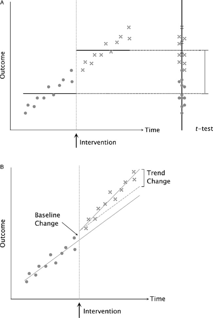
Panel A contains artificial data with an annotated intervention. Bullet points denote pre-intervention measurements, crosses indicate post-intervention measurements. The horizontal lines correspond to the group means for pre- and post-intervention. The right panel of the figure contains the projection of the time-series to illustrate a t-test. As shown in Table 1, the t-test yields a highly significant result for a difference between the means of the two groups capturing the secular trend instead of the intervention impact. Panel B contains a different artificial dataset with the ITS regression lines. The dashed line indicates the secular trend corrected for the baseline change
Panel B of Figure 1 contains a new data set with an intervention affecting the outcome. An ITS is a segmental linear regression model; pre-intervention and post-intervention are each modeled as a linear regression. 3 Based on an ITS, a secular trend can therefore be captured in the regression line as shown in panel B of Figure 1. An ITS compares the intercept and slope of the regression line before the intervention with the intercept and slope after intervention. A one-time baseline effect of the intervention without influencing the secular trend can be detected as an intercept change. If the intervention changed the secular trend, there will also be a significant difference in the slope between the two periods. Later, we will see that an ITS also comprises more flexible models.
Instead of using an ITS design, many studies use pre- and post-intervention groups without modeling the secular time trend. Examples include evaluations of major interventions to improve financial protection in healthcare systems, such as universal coverage in Taiwan, 4 or the introduction of drug prescription benefits in US Medicare, 5 an evaluation of pay for performance programme in the UK 6 and an assessment of the benefits of improved sanitation in rural India. 7 While these examples highlight the scope for greater use of ITS in evaluation research, it is important that this methodology is applied correctly and to appropriate situations. 8
Methodology
In this section, we introduce ITS understandable to a non-statistical audience. We start by describing the main features of the ITS. Next, we present the ITS model in more detail and finish with advice about interpretation of results.
Data and Effects
A dataset for an ITS contains data points before and after the intervention. Each time point can have multiple measurements, which can be shown as aggregated measurements. Often, the spatial dimension introduces multiple measurements, for example measurements for a health indicator in different regions. Technically, the minimum data requirements for an ITS are three measurements before and three measurements after the intervention to ensure suitable estimation of standard errors. 9 The measurements have to be distributed on at least two time points before and two time points after the intervention such that the trends of the measurements before and after the intervention can be estimated. More measurements and time points are strongly recommended, especially for data with high variance. As a rule of thumb, we recommend to use at least three measurements per time point. Furthermore, we assume that the time of intervention is known, as is commonly the case with health care interventions. Autoregressive integrated moving average (ARIMA) models or change point models may be appropriate to estimate the time of the intervention when it is not known.10,11
In this article, we restrict our discussion to univariate outcome measures. The intervention can have two main effects on the outcome. Firstly, the intervention baseline effect is a change of baseline between pre- and post-intervention. This is observed as a gap between pre- and post-intervention. Secondly, the intervention trend effect occurs if the intervention changes the slope of the fitted regression line after the intervention.
ITS Model
An ITS is a regression model with an intervention at a given time point. The intervention splits the regression into the two segments pre- and post-intervention such that we can employ a modified segmented linear regression model. 12 In the simplest case, a regression line models each segment individually. A regression line is a line, which fits best to the data. Minimizing the mean squared distances of the points to the line optimizes the fit. A regression line is defined by a coefficient for the offset and for the slope. Technically, the first regression line is fitted to both pre- and post-intervention data. The offset reflects the overall baseline of all data points. The slope corresponds to the secular trend. To allow for an effect of the intervention, a second line is fitted simultaneously capturing the deviation of the post-intervention data from the first line. The simultaneous fitting procedure ensures that the sum of both lines optimally fit the data. Thus, the first line is not influenced by deviations of the post-intervention data but describes the secular trend over the whole time.
Similar to the setup for the t-test, we can compare the pre- with the post-intervention group. In contrast to a t-test, we can isolate the effect of the intervention from the secular trend. The coefficient for the offset of the post-intervention line corresponds to the baseline change. Based on a test, we can obtain a P-value for the null hypothesis that the coefficient is unequal to zero. For a sufficiently small P-value, we consider the difference significant and conclude that the outcome changed significantly upon intervention. Similarly, we can test the coefficient of the slope of the post-intervention line representing the deviation from the secular trend. If the slope is significantly different from zero, the outcome trend over time changed upon intervention. As we will see later, both conclusions do not necessarily imply that the intervention caused the change of the outcome.
More complex models with non-linear time effects or lagged time effects can also be developed. A more complex model will obtain a better fit of the data due to the increased flexibility or the so-called degrees of freedom. However, this may not be desirable because it decreases general-izability How do we choose an adequate model? One can use the pre-intervention measurements to choose a reasonable model. It is good practice to test if coefficients for more complex model features like quadratic time effects are significantly different from zero. In this case, one can further justify the more complex models by comparison with the simpler model based on Bayesian Information (BIC) or Akaike Information Criterion (AIC), which both penalize model complexity.
Interpretation
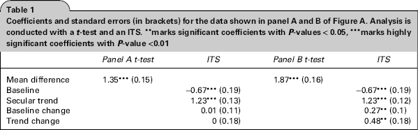
The results of the ITS are usually summarized as in Table 1, reporting coefficients and standard errors. The standard error indicates the uncertainty of the estimated coefficient. As a rule of thumb, two times the standard error to either side of the estimated coefficient corresponds to the 95% confidence interval. If this interval contains zero, we cannot reject the null hypothesis that the coefficient is zero on a 5% confidence level. Table 1 shows the results for a t-test and for an ITS for the data in Figure 1 panel A and panel B. The t-test for panel A data is highly significant because the secular trend is captured as difference between pre- and post-intervention. In contrast, the ITS for this dataset does not allow us to reject the hypothesis as the outcome measure does not change upon intervention. Often, ITS results are separately reported for baseline, secular trend, baseline change upon intervention and trend change upon intervention. The coefficient for baseline is usually significant if the data is not normalized to a zero mean. A secular trend leads to a significant coefficient for the trend coefficient. This is an indicator that a t-test is likely to be prone to false positives or false negatives depending on the sign of the coefficient. In terms of impact evaluation, the baseline change coefficient corresponds to a one-time effect upon intervention and the trend change indicates a lasting effect on the outcome. Thus, if any of the two ‘change’ coefficient is significantly different from zero, the outcome changed with the onset of the intervention. In the next section, we will discuss why this does not always imply a causal relation.
Coefficients and standard errors (in brackets) for the data shown in panel A and B of Figure A. Analysis is conducted with a t-test and an ITS. **marks significant coefficients with P-values < 0.05, ***marks highly significant coefficients with P-value <0.01
Discussion
The ITS design can help to overcome spurious detection of effects due to the underlying secular trends of the data. The key difference to the RCT design is that exposure to an intervention is not determined by randomization and there is no control group. In an RCT, theoretically the control group only differs from the treatment group by the treatment, although the randomization process does not always produce equivalent groups. Therefore, other external influences, which affect the outcome, are incorporated in the control group effect. The difference between the control and treatment group cancels out such effects; both groups only differ with respect to treatment.
In an ITS design, we do not observe a control group. Instead, we assume that the outcome would have evolved according to the secular trend if no intervention had been present. It is important to note that this assumption is violated if the post-intervention outcome is subject to additional external influences. An ITS design cannot distinguish between the effect of the intervention and external influences affecting the outcome specifically in the pre- or post-treatment group. This results in two main caveats. Firstly, the change in the outcome might not be expected to stay constant even in the absence of an intervention. An assumed linear trend would yield false negative or false positive results. Secondly, parallel interventions cannot be disentangled. As legislative regulations are often introduced at one time point, different changes accumulate at specific dates. Furthermore, other regulations can have unintended side effects.
For example, in the context of package size restrictions of paracetamol to decrease deaths from poisoning, an ITS analysis detects significant effects on the reduction of poisoning deaths. However, comparing the intervention trend change to that with fatal poisonings associated with other medications, such as aspirin and antidepressants not subject to package size restriction, suggests that external influences rather than this intervention may be the real cause. 13 The regulations might have raised the general awareness amongst physicians prescribing antidepressants and amongst retailers selling drugs such as paracetamol and aspirin to specific target groups like young girls.
In conclusion, ITS design helps to distinguish time effects from intervention effects. It is very helpful for the analysis of healthcare policies, which are introduced without a control group. However, an ITS analysis cannot exclude external influences co-occurring with the intervention as this conceptually requires a control group.
Summary Points
Standard statistical tests (e.g. t-tests) do not consider underlying secular trends in the data. A linear secular trend increases the difference between two groups divided by an intervention. For interventions without an effect on the outcome, the linear trend can yield a significant but spurious difference. The intervention erroneously appears to have a significant effect on the outcome.
An ITS design allows secular trends in the model. Therefore, the effect of the intervention is only significant if the trend changes at the intervention or the intervention shifts the outcome up or down.
The standard ITS design assumes that the measurements are independent. Often, measurement errors accumulate such that measurements are auto-correlated, which violates above assumption. This can bias the estimator for the standard error The Durbin-Watson test can be used to detect auto-correlation. If auto-correlation cannot be rejected, the ITS model can be extended by an additional effect for auto-correlation.
The assumed secular trend is crucial for identification of an intervention effect. An erroneously assumed linear trend can yield false positives and false negatives. The choice of the secular trend should be estimated and tested based on the pre-intervention data and motivated by underlying characteristics of the outcome.
An ITS design cannot distinguish between the effect of the intervention or any other co-occurring events at the same time. Therefore, authors should discuss the possibility of other simultaneous effects on the outcome. As in the study of the paracetamol package size restriction, it can be crucial to investigate simultaneous effects by analyzing outcomes not affected by the intervention.
A technical appendix is available at http://jrsm.rsmjoumals.com/lookup/suppl/doi:10.1258/jrsm.2012.110319/-/DC1, the code files can be accessed at http://jrsm.rsmjournals.com/lookup/suppl/doi:10.1258/jrsm.2012.110319/-/DC2
Footnotes
Acknowledgements
We thank Oliver Morgan for supplying the data used in the paracetamol example