Sage Journals: Discover world-class research

Abstract

Background

Reference intervals are used to distinguish between healthy and diseased state. Ideally, they are defined using specimens only from ‘healthy’ individuals, but this is often difficult or impossible. In order to use routine clinical laboratory data, outliers must be removed before the underlying distribution and changes related to age and sex can be modelled. This paper illustrates the process for plasma alkaline phosphatase (ALP). ALP levels are high in infancy and childhood, peak in adolescence, are stable from the early 20s and rise after the fourth decade. Three types of normalizing transformations (Logarithmic, Box-Cox and Cole's LMS) are compared.

Methods

Single ALP results from 75,328 individuals aged 0–80 years were binned by sex and age. The normalizing transformations were applied to each bin, outliers were removed and the normalizing transformations were reapplied to the remaining data. The normality of the transformed data was assessed by normal score plots and the Kolmogorov-Smirnov test. Fractional polynomials were used to model the underlying parameters of the transformations and the derived parametric reference intervals (mean ± 1.96 standard deviations), separately for each sex as a whole and partitioned into two or three age ranges, with overlapping to give smooth transitions.

Results

All transformations yielded acceptably normal data, but the LMS method gave the closest approximation to normal. Outlier rates were similar for each method. The derived reference ranges were similar for all the three methods. Splitting the data-set into several segments resulted in a better fit with the peak seen in adolescence.

Conclusion

Routine clinical laboratory specimens can be used to derive reference intervals.

Introduction

In clinical practice, reference intervals for laboratory tests are used to distinguish between healthy and diseased individuals, and to define the expected values in healthy individuals. They commonly incorporate the lower or middle 95% of values from subjects of a defined population. Ideally, the specimens used to define reference intervals should be collected from subjects known to be healthy. This is rarely practicable as there is often no easily identifiable population available and, for analytes such as alkaline phosphatase (ALP) in which substantial changes occur with age, several thousand specimens may be required. Another approach is to use specimens from patients, most of them having a low prior likelihood of an ‘abnormal’ value for the parameter of interest. The process has three steps:

Identify and remove outliers;

Define the underlying distribution of the remaining data points, stratified if necessary by age and sex;

Model the effects of variables such as age and sex.

This paper illustrates the use of this process to derive reliable reference ranges using specimens received by a routine clinical biochemistry laboratory for ALP, a plasma enzyme that shows large variations related to age and sex. Three methods are compared for transforming the data to obtain approximately normal distributions.

Methods

Alkaline phosphatase

The method for measuring plasma ALP is a standard kinetic chemistry procedure followed by the production of a coloured product spectrophotometrically, p-nitrophenol on the Abbott Aeroset (Abbott Instruments, Maidenhead, Berkshire, UK).¹ Specimens in which ALP is measured are almost exclusively heparinized plasma.

Data-set

The laboratory is a general clinical chemistry laboratory based in a teaching hospital and receives specimens from primary, secondary and tertiary care. The laboratory information system was used to identify all specimens from males and females aged 0–80 years with an ALP measurement over a period of one year. In subjects with more than one measurement, the earliest result was used. Age at the time of the first measurement was rounded down to whole years. Sex was also recorded.

Statistical methods

Data were analysed using the R statistical computing environment (version 2.60)² running on a G4 Apple Powerbook and an Intel Apple Macintosh iMac under OS X (version 10.5, Apple, Cupertino, CA, USA). The data were grouped (‘binned’) by age and sex. The two sexes were analysed separately.

The effects of three data transformations to make the distribution approximately normal (normalizing transformation) were examined. After an initial normalizing transformation using all the data, outliers were excluded, and the remaining data were transformed again using the three methods. The transformed data were used to define reference intervals and these were modelled using fractional polynomials.³

Normalizing transformations

Three normalizing transformations were used.

Logarithmic transformation:

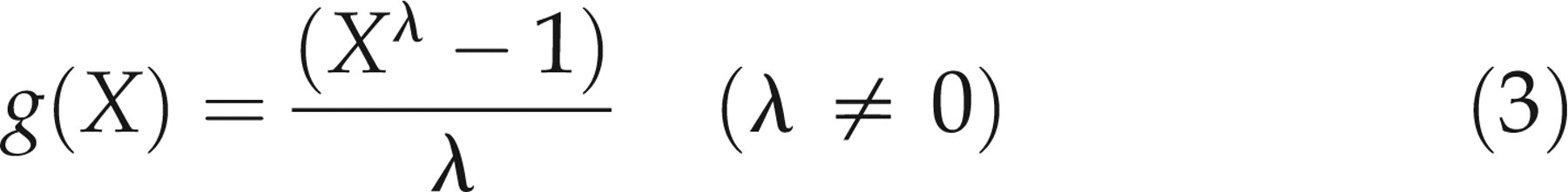
where log(X) is the natural logarithm (to base e). The constant c was taken to be zero.

Box-Cox transformation: The Box-Cox transformation uses a single parameter, λ:⁴

The logarithmic transformation is thus a special case of the Box-Cox transformation.

For the Box-Cox transformation, the best value of λ for each age–sex combination was found by estimating the likelihood of the fit for all values between −1 and +1 in steps of 0.05, and using the value with the maximum likelihood.

Cole's LMS method:⁵ Cole's method also uses a Box-Cox transformation and consists of estimating the three parameters: shape (L – equivalent to λ in the Box-Cox distribution), untransformed geometric mean (M) and modified standard deviation (SD) or coefficient of variation of the transformed data (S) for each age–sex group, using a standard formula to estimate L. These are then fitted using a suitable method, and the parametric reference intervals are derived by back-transformation of the mean ± 1.96 SDs to give the 2.5 and 97.5 percentile values.

Outlier detection and exclusion

The initial parameters were set for each bin using all the data for that bin. Outliers in each bin were detected using an adaptation suggested by Horn et al. ⁶ of the method described by Hoaglin et al. ⁷ Following the normalizing transformation, the upper (Q1) and lower (Q3) quartiles and the interquartile range (IQR: Q1 – Q3) of the transformed data were calculated for each bin. Specimens were excluded if they lay outside the interval (Q1 − 1.5 × IQR) to (Q3 + 1.5 × IQR). The proportion of results excluded from each bin was compared graphically between methods. The parameters for each transformation were recalculated excluding the values identified as outliers. These parameters were then used to identify and exclude outliers from the whole data-set.

Fitting of reference intervals using included specimens

For the logarithmic fit, the transformed means and SDs for each bin were fitted using fractional polynomials, and the derived values for the mean ± 1.96 SDs were back-transformed to provide reference intervals. For the Box-Cox method, the parametric reference intervals were derived for each bin and then fitted using fractional polynomials. For the LMS method, the geometric means of the raw values (M), shape parameter (L) and transformed coefficient of variation (S) were fitted using fractional polynomials and the reference intervals were derived using the three fitted values. In each case, stepwise regression was used to fit fractional polynomials with powers of age from −3 to +3 in steps of 0.5, using the Aikike Information Criterion to decide on the effect of adding or removing terms.³ For each method, the effects of fitting the data in one (0–80 years), two (0–15, 15–80) or three (0–11, 11–17, 17–80) age segments were compared. Adjoining segments were fitted by overlapping three years and using the mean of the two fits for the overlapping segment.

The reference intervals were plotted against the non-parametric raw values for the 2.5 and 97.5 percentiles using the data after exclusion of outliers.

Model checking

Outlier rejection was assessed by checking the proportion of values rejected by each method.

The effect of normalizing transformations was assessed by plotting normal probability for the transformed SD values of included values, by calculating the skewness and kurtosis, and by the Kolmogorov-Smirnov (KS) test against a normal distribution. The KS test is a general test for the equality of two distributions, which makes no assumptions about their shape.

The differences between the raw non-parametric and fitted parametric intervals were examined by plotting the percentage difference between the values against age, by calculating the mean and SD of the mean percentage difference, and by calculating the proportion of fitted values within 10% of the raw values. The percentage differences in the upper limits calculated by each method for age were plotted as histograms.

Other data-sets

Two other data-sets were examined:

The laboratory data-file from the United States Third National Health and Nutrition Examination Survey (NHANES III);⁸

A laboratory data-set from 2007 following a further change of analyser in 2006.

Results

The initial data-set consisted of 109,000 results from 86,542 subjects (45,861 females, 39,412 males), of which 3483 specimens were excluded because the age and/or sex were missing, and 7729 specimens where the age was >80 years. The analysis was conducted on the remaining 75,328 specimens (35,684 males). The age and sex distributions of the data are shown in Figure 1.

Figure 1

Age and sex distribution of specimens for alkaline phosphatase measurements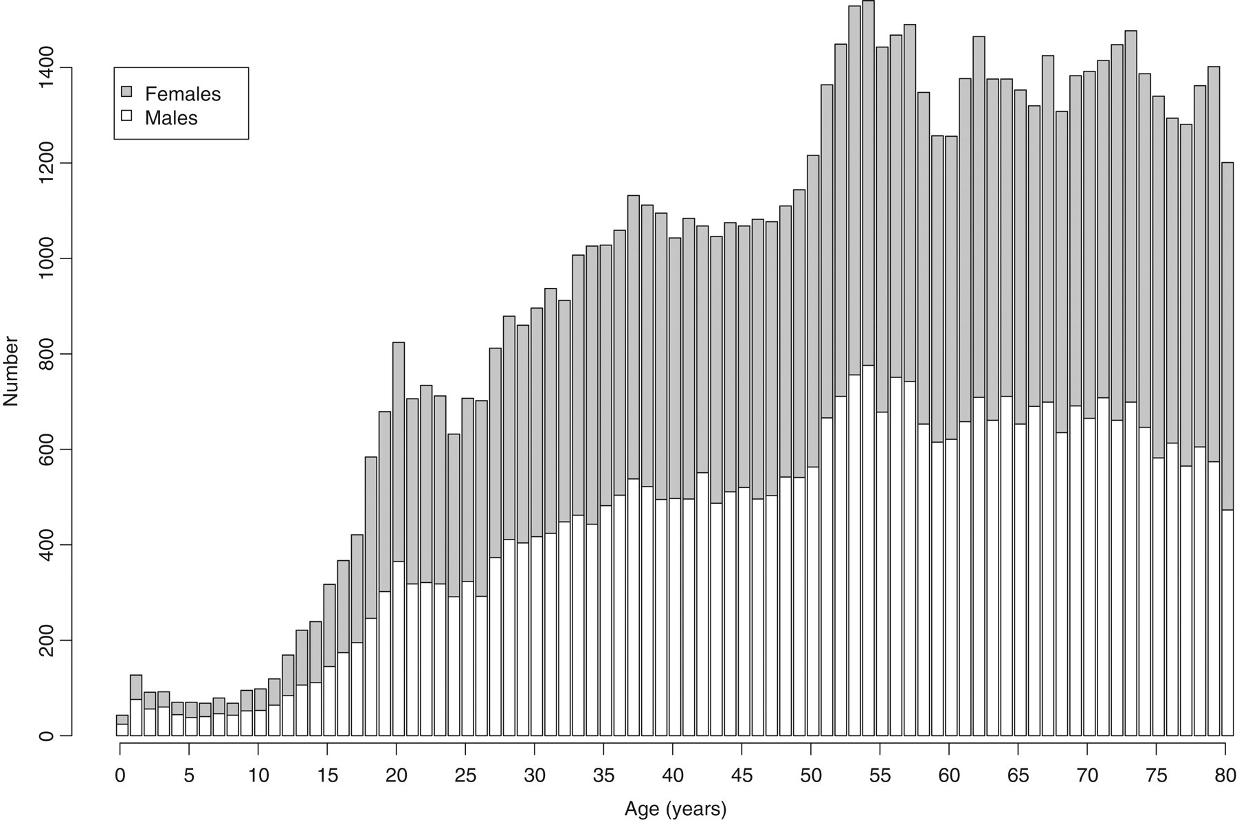

Exclusion of specimens

The proportion of specimens rejected was similar overall for the Box-Cox and Cole methods (2.93% and 2.98%, respectively, and greatest for the logarithmic transformation [3.66%]). More outliers were detected in the data from young subjects than from older subjects (Figure 2), and the logarithmic transformation resulted in larger proportions of older subjects being rejected than with the other two methods.

Figure 2

Rejection rates for the three transformations vs. age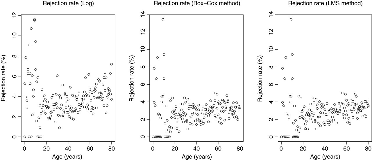

Normalizing transformations

Figure 3 shows normal scores plot for untransformed and transformed ALP values. The SD scores represent the aggregated data using values normalized within each bin separately. The SD score of a datapoint is calculated by taking the mean of the transformed values for the bin from the value and dividing by the SD of the values of that bin. The graph plots the normal scores against the normal scores expected for a normal distribution. A normally distributed data-set should give a straight line. Panel A shows the raw data without exclusions (skewness 7.3, kurtosis 94). The positive skewness is shown by the line being non-linear and concave upwards. This shows that the normal scores obtained are lower than would be expected, showing a concentration of low values and a long ‘tail’ of high values. After exclusion of outliers, logarithmic transformation resulted in a much improved although not perfect normal distribution with skewness and kurtosis 0.15 and 2.87, respectively (Panel B, Figure 3). The Box-Cox (Panel C, skewness 0.004, kurtosis 2.87) and LMS (Panel D, skewness 0.05, kurtosis 2.84) transformations resulted in more normally distributed transformed data after exclusion of outliers, especially at higher values. These impressions were confirmed by the KS test for equality of distributions, which showed that all three transformations differed from a normal distribution, least for the LMS method (P = 0.02) compared with Box-Cox method (P = 0.006), and most for the logarithmic transform (P < 0.0001). However, although these are statistically significant, inspection of the normal scores plot suggests that each of the fits is acceptable.

Figure 3

Normal score plots for raw data (with no exclusions), and for different transformations with exclusion of outliers. Normally distributed data should yield a straight line. All transformations show some non-linearity indicating some lack of fit, least for the LMS method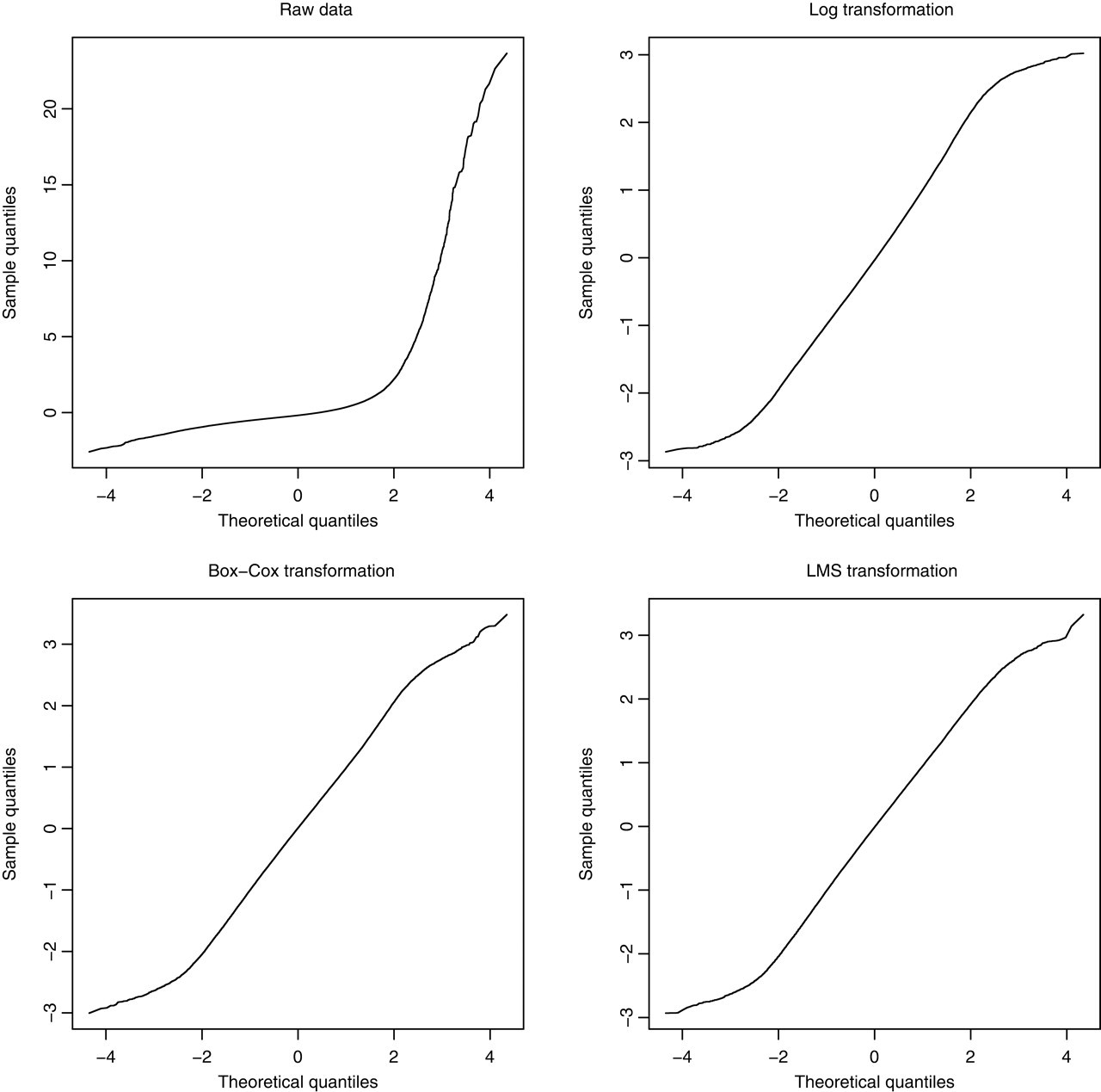

Comparison of fitted data

Fractional polynomial fits with exponents between −3 and +3 provided good fits to the data for all three transformations, including the peaks in infancy and puberty with similar reference intervals. Dividing the data into two (0–15, 15–80) or three (0–11, 11–17, 17–80) age segments gave better fits to the peak around puberty, and a more linear fit to the data after 20 years of age for all the transformations. These are shown in the case of the logarithmic fit (Figure 4).

Figure 4

Raw non-parametric (2.5 and 97.5 percentiles) and fitted parametric reference intervals (mean ± 1.96 SDs) for alkaline phosphatase using logarithmic normalizing transformation, showing effects of fitting the data using a single segment for all ages, two segments (join at 15 years) and three segments (join at 10 and 15 years)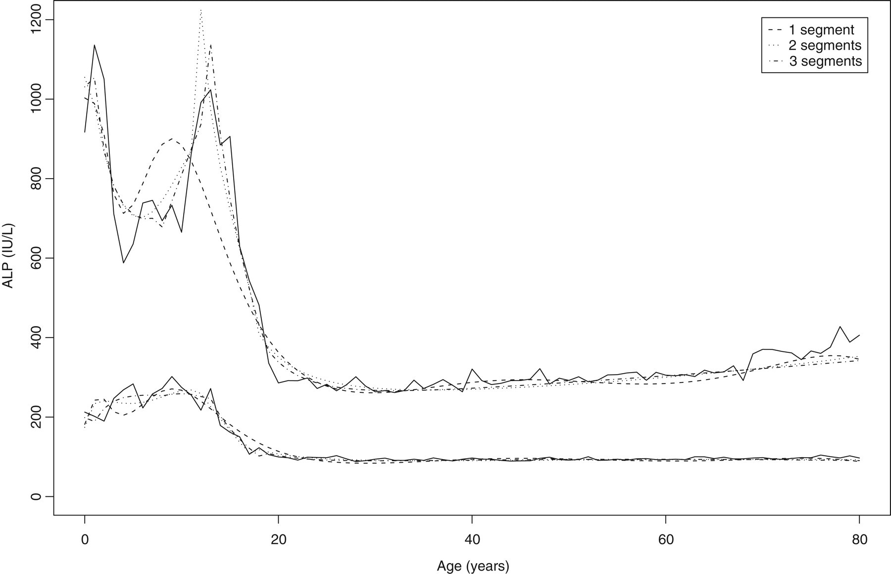

There was overall good agreement between the raw and fitted values: the mean deviation (±SD) of the upper limit of the reference interval was −2.2 (9.3)% for the logarithmic transformation, 0.5 (13.5) for the Box-Cox transformation and 0.9 (12.8) for the LMS method. All transformations performed fairly well, but with some outliers. A total of 78% of fitted values were within 10% of the raw values for the logarithmic transformation compared with 60% for the Box-Cox transformation and 65% for the LMS method. The tighter distribution of the logarithmic fit is shown in Figure 5, in which the percentage difference of the fitted values for each of the transformations is plotted by the number of fitted segments against the age of the subjects. This shows that all of the fits deviated somewhat from the non-parametric fits during the adolescent peak, and in infancy, but with fairly stable values for adults.

Figure 5

Percentage differences between raw and fitted upper limits for three transformations (Logarithmic, Box-Cox and LMS) comparing one-, two- and three- segment fits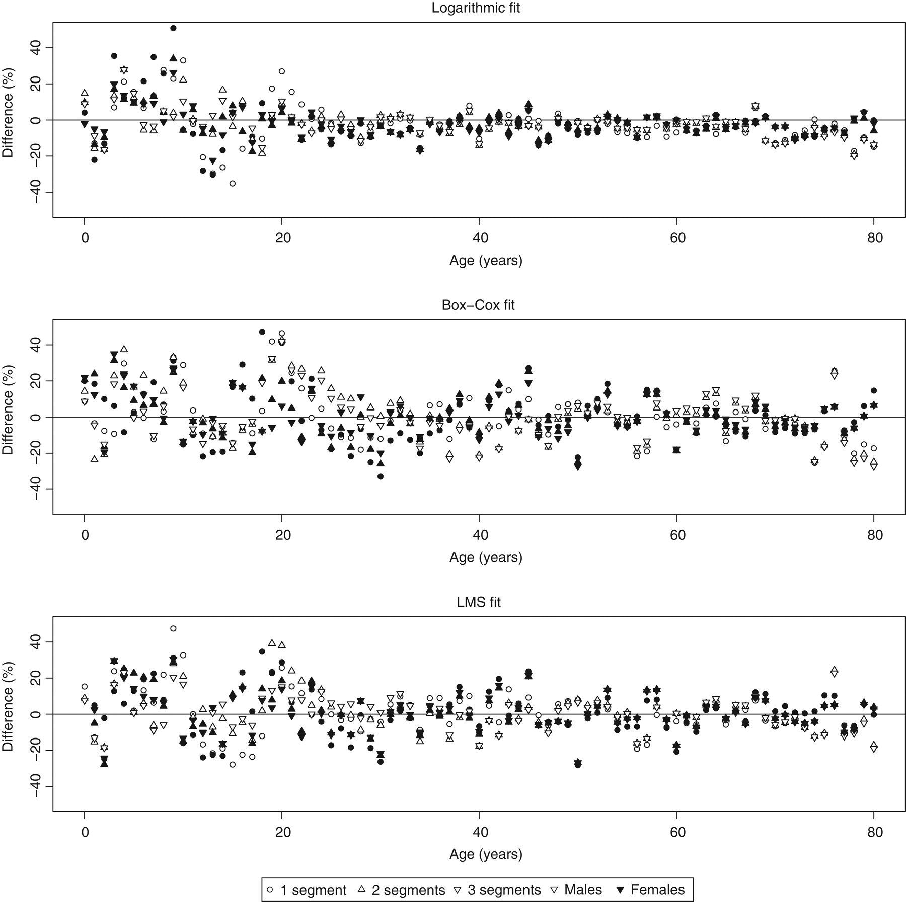

The fitted limits were similar for all the three methods (Figure 6), although the logarithmic fit gave lower upper limits for older adults. The exclusion rate was greater for the logarithmic transformation for older age groups, and this is probably responsible for the narrower reference ranges produced by this fit. The LMS and Box-Cox transformations gave upper limits that were very similar (mean difference −0.1 ± 7.1%), but higher than the logarithmic transformation (11.1 ± 9.2 for LMS, 11.4 ± 11.5 for Box-Cox).

Figure 6

Comparison of non-parametric limits for logarithmic transformation and LMS method, and of the fitted parametric limits using logarithmic, Box-Cox and LMS method using three segments (join at 10 and 15 years)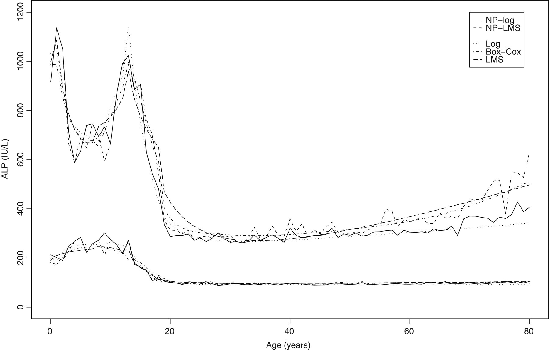

Fitting of other data-sets

The same methods were applied to fitting ALP values from the NHANES III data-set, which is publicly available, and to more recent data after a further change of analyser in 2006. The NHANES data-set contains ALP values for some 29,000 subjects aged 12–90 years. The more recent laboratory data-set contained results for 132,210 patients aged 0–80 years. The results of all the fits were similar.

Discussion

In clinical laboratories, reference intervals for laboratory tests are commonly defined as the central 95% of values expected from ‘healthy’ individuals. This may be useful in diagnosis, although the majority of specimens received by laboratories are for other purposes, such as monitoring disease progression or checking for the intended or adverse effects of interventions. In these situations, ‘healthy’ reference intervals may have less utility, although the expected values associated with disease or adverse effects of treatment may be known. Defining reference intervals is often a problem for clinical laboratories, because it may be difficult to obtain adequate number of specimens from ‘healthy’ volunteers, and the reasons for collecting clinical specimens increase the likelihod of obtaining values outside the reference interval. Although the majority of assay specimens are likely to have results within acceptable limits, there will be a subset with abnormal levels in the data distribution. This problem can be circumvented to some extent by the use of presumed healthy subjects, as with large-scale surveys such as NHANES.^9,10 These studies provide valuable data on the distribution of values expected in healthy subjects. However, these surveys are not without problems of bias, as a subset of the subjects will be unhealthy and may bias the results of the overall sample unless outlers are identified and excluded. It is also possible to use hospital database data to obtain reference intervals.¹¹

A preliminary trawl of the data may enable removal of values for individuals with a high likelihood of disease affecting the parameter of interest. There are three steps in generating reference intervals:

Identify and remove outliers;

Identify and model the underlying distribution of values using an appropriate transformation, subdivided if necessary into bins defined by age and sex;

Identify and model the effects of factors such as age and sex.

Outliers are defined as values that do not belong to the reference population. If not identified, they widen the reference interval. Methods for dealing with the effects of outliers on reference intervals are reviewed by Horn et al. ⁶ It is possible to reduce the effect of outliers using robust estimators for the reference interval, for instance by using non-parametric methods or a normalizing transformation (such as the Box-Cox transformation). The Clinical and Laboratory Standards Institute has suggested using a normalizing transformation followed by a method to remove kurtosis.¹² The method proposed by Horn et al. ⁶ was used to remove outliers. Each transformation was used to give an initial normalization of the data. Outliers were removed by using limits based upon the IQR and the upper and lower quartiles. This should remove the effect of outliers, although Horn's group has pointed out that this will tend to give limits that are too narrow, and that the range of data should probably be inflated by approximately 0.7%.

Although any distribution can be used to fit data, normally distributed data are attractive because they are relatively easy to work with. Biological data often have a non-normal distribution, even after removal of outliers. Two important sources of non-normality are skewness and kurtosis. Skewness refers to asymmetry, and is called positive if there is a long tail of high values on a histogram. Kurtosis is the tendency for the tails of a symmetrical distribution to include fewer (increased kurtosis) or a greater number of observations than expected in a normal distribution. The two quantities can be measured by dividing the third (skewness) and fourth (kurtosis) moments about the mean by the cube and fourth power of the SD of the data. Mathematically, these are:

and

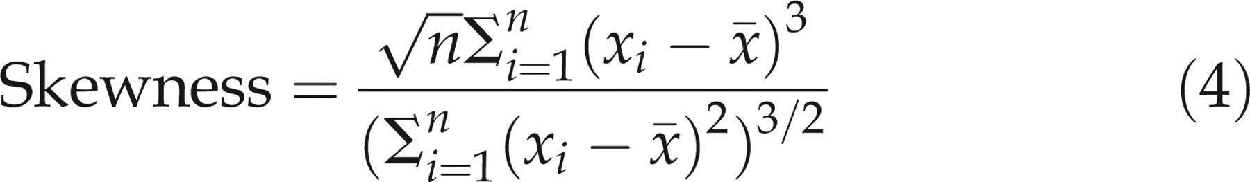
For normally distributed data, the expected values are 0 for skewness and 3 for kurtosis.

Normalization of data is often difficult and approximate. The Box-Cox family of transformations, especially the logarithmic transformation, often results in an approximately normal distribution. The IFCC Expert Panel on Theory of Reference Values (EPTRV) has suggested trying other transformations,¹² such as the square root transform or a two-stage transform, in which the first stage (e.g. an exponential transform) removes skewness:

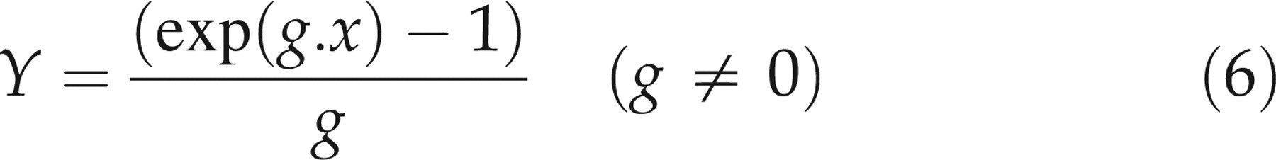
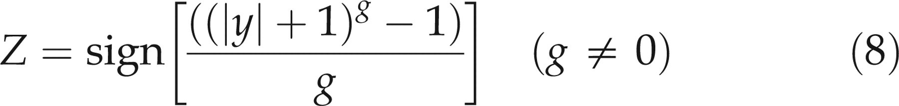
and the second (e.g. the modulus transform of John and Draper) removes kurtosis:

For this study, only the Box-Cox family of transformations was used. All three transformations (logarithmic, Box-Cox and Cole LMS method) yielded fairly good approximations to a normal distribution as judged by normal quantile plots of the binned normal deviates following outlier removal (Figure 3), although the Cole method provided the best approximation to normality with only moderate non-normality.

The final step is to model the age- and sex-related levels. This may be complicated in the case of analytes such as ALP that show pronounced age-related changes. The main sources of plasma ALP activity are usually liver and bone, with smaller contributions from intestine, placenta and kidneys. Higher levels of ALP are associated with increased bone turnover (growth, repair of fractures, thyrotoxicosis and metastatic malignant disease with spread to bone) and liver disease, especially biliary obstruction. ALP levels are higher in childhood and adolescence because of increased bone turnover associated with growth. During adulthood, the levels of bony ALP increase slightly with age – more in women, especially after the menopause – and this is thought to reflect increased bone turnover.

Many methods have been proposed for modelling the derived reference intervals (reviewed by Wright and Royston).¹³ While polynomials using integer powers of the independent variable (age in this case) are popular, models derived from them are not flexible. It is also possible to use spline functions. A spline was originally a flexible piece of wood, plastic or metal used for drawing smooth curves, and such devices were widely employed for drawing calibration curves before computers were routinely available for fitting the data. However, Royston and Altman¹⁴ suggested that splines are often more complex than necessary for the task of defining reference intervals and have the major drawback that, ‘since they use local models, they do not yield simple equations for prediction’. Therefore, they proposed using fractional polynomials as they are ‘reasonably flexible, easy to understand, parsimonious, and perhaps, above all, are simple and quick to fit using standard multiple-regression software’. In this study, the method suggested by Wright and Royston using fractional polynomials was used.³ Two approaches are possible:

Modelling the parameters such as the shape (λ), the mean and a measure of variation, such as SD;

Modelling the derived reference values.

The first method worked well with the logarithmic and LMS methods, but not with the Box-Cox approach. For all methods, it was possible to use fractional polynomials to model the values for the intervals derived from individual bins. This approach has the advantage of making fewer assumptions about the homogeneity of variance between bins. In the end, all the methods yielded very similar reference intervals, and the percentage differences between the raw and fitted values were mostly small and clinically insignificant. The higher rate of outlier detection for the logarithmic method resulted in narrower reference intervals in older age groups. Overall, the derived intervals were slightly different from historical reference intervals used by the laboratory,¹⁵ but differed significantly from those published by the manufacturer,¹⁶ citing,¹⁷ especially for children (Table 1). Further investigation revealed that comparison between the unmodified Aeroset method and our previous method had shown a positive bias of about 10 U/L but the laboratory's reference intervals had not been changed.

Table 1

Reference intervals (in U/L) from manufacturer's method package insert (Insert), laboratory standard operating procedure (SOP) and adopted reference intervals

Age group	Cases	Insert	SOP	Adopted
Males
0–3	183	<500	150–570	200–1100
3–10	295	<500	150–570	250–720
10–15	507	<750	150–570	210–1000
15–19	898	Not given	80–250	110–700
19–40	8428	40–150	80–250	95–280
40–60	11793	40–150	80–250	95–290
60–80	12482	40–150	80–250	95–320
Females
0–3	114	<500	150–570	200–1100
3–9	226	<500	150–570	240–750
9–15	549	Not given	150–570	120–950
15–20	1094	40–150	80–250	85–300
20–40	9895	40–150	80–250	75–250
40–60	12567	40–150	80–250	80–290
60–80	14000	40–150	80–250	100–330

Dividing the data into segments improved the model fit to the raw data (Figure 4). The discontinuities at the junctions between adjacent age segments were handled using the means of the derived points.

None of the methods was very complex, although the logarithmic transformation was simplest. Comparison of the logarithmic and LMS methods shows that the end results were very similar, and the logarithmic method would therefore be satisfactory in practice.

In summary, this work shows that:

Reference intervals based on historical values and manufacturers' recommendations should be checked when new analysers are commissioned;

It is possible to use routinely collected laboratory data to derive valid reference intervals;

If there is significant heterogeneity, the data should be divided into convenient bins based on age and/or sex;

A normalizing transformation for each bin allows identification and removal of outliers;

Following removal of outliers, the normalizing transformation can be refined using the remaining data points;

Parameteric reference intervals can be derived by fitting the normalizing parameters, and then the means and SDs or the derived reference interval for each bin using a method such as fractional polynomials;

More complex transformations may provide better normalization and fits to data, but simple transformations such as logarithmic transformations often yield satisfactory results, in terms of deviation from the raw values and differences from the results of other fits;

Dividing the data into segments may simplify the models, but may result in discontinuities, which can be dealt with by overlapping the segments and averaging the fitted values.

References

Tietz

, Rinker

, Shaw

. IFCC methods for the measurement of catalytic concentration of enzymes. 5. IFCC method for alkaline-phosphatase. J Clin Chem Clin Biochem 1983;21:731–748

R Development Core Team. R: A Language and Environment for Statistical Computing Vienna, Austria: 2007. ISBN 3-900051-07-0. See http://www.R-project.org (accessed 16 May 2008)

Royston

, Altman

. Approximating statistical functions by using fractional polynomial regression. Statistician 1997;46:411–422

Box

GEP

, Cox

. An analysis of transformations revisited, rebutted. J Am Stat Assoc 1982;77:209–210

Cole

, Green

. Smoothing reference centile curves: the LMS method and penalized likelihood. Stat Med 1992;11:1305–19

Horn

, Feng

, Li

, Pesce

. Effect of outliers and nonhealthy individuals on reference interval estimation. Clin Chem 2001;47:2137–45

Hoaglin

, Iglewicz

, Tukey

. Performance of some resistant rules for outlier labeling. J Am Stat Assoc 1986;81:991–999

CDC. Third National Health and Nutrition Examination Survey (NHANES III) [http://www.cdc.gov/nchs/nhanes.htm (accessed 16 May 2008)]

Cembrowski

, Chan

, Bamforth

. NHANES 1999–2000 data used to create comprehensive health-associated adolescent reference intervals for 21 chemistry analytes measured by the Hitachi 704. Clin Chem 2004;50:A126

10.

Cembrowski

, Chan

, Zhang

. Third NHANES used to create comprehensive healthassociated reference intervals for 21 serum chemistry analytes measured by the Hitachi 737. Clin Chem 2001;47:A118

11.

Kouri

, Kairisto

, Virtanen

, Uusipaikka

, Koivula

, Nanto

. Reliability and adequacy of discharge diagnosis databases in the production of reference values. Scand J Clin Lab Invest 1995;55(Suppl. 222):69–73

12.

Solberg

. Approved recommendation (1987) on the theory of reference values. 5. Statistical treatment of collected reference values – determination of reference limits. Clin Chim Acta 1987;170:S13–S32

13.

Wright

, Royston

. A comparison of statistical methods for age-related reference intervals. J Roy Statist Soc Ser A – Stat Soc 1997;160:47–69

14.

Royston

, Altman

. Regression using fractional polynomials of continuous covariates – parsimonious parametric modeling. Appl Stat – J Roy Statist Soc Ser C 1994;43:429–467

15.

James

, Draisey

, Kirby

, Cox

. Internal SOP 1/A/3 R1 v4.doc; 2004

16.

Abbott Laboratories. Alkaline phosphatase 7D55-20 and 7D55-30 30-3947/R7. Abbott Laboratories, Abbott Park, IL, USA; 2007

17.

Moss

, Henderson

. Clinical Enzymology. In: Burtis

, Ashwood

eds. Tietz Textbook of Clinical Chemistry. 2nd edn. Philadelphia, PA: WB Saunders, 1994: p. 836

Use of routine clinical laboratory data to define reference intervals

Abstract

Background

Methods

Results

Conclusion

Introduction

Methods

Alkaline phosphatase

Data-set

Statistical methods

Normalizing transformations

Outlier detection and exclusion

Fitting of reference intervals using included specimens

Model checking

Other data-sets

Results

Exclusion of specimens

Normalizing transformations

Comparison of fitted data

Fitting of other data-sets

Discussion

References