
Abstract
X-ray computer tomography (CT) is fast becoming an accepted tool within the materials science community for the acquisition of 3D images. Here the authors review the current state of the art as CT transforms from a qualitative diagnostic tool to a quantitative one. Our review considers first the image acquisition process, including the use of iterative reconstruction strategies suited to specific segmentation tasks and emerging methods that provide more insight (e.g. fast and high resolution imaging, crystallite (grain) imaging) than conventional attenuation based tomography. Methods and shortcomings of CT are examined for the quantification of 3D volumetric data to extract key topological parameters such as phase fractions, phase contiguity, and damage levels as well as density variations. As a non-destructive technique, CT is an ideal means of following structural development over time via time lapse sequences of 3D images (sometimes called 3D movies or 4D imaging). This includes information needed to optimise manufacturing processes, for example sintering or solidification, or to highlight the proclivity of specific degradation processes under service conditions, such as intergranular corrosion or fatigue crack growth. Besides the repeated application of static 3D image quantification to track such changes, digital volume correlation (DVC) and particle tracking (PT) methods are enabling the mapping of deformation in 3D over time. Finally the use of CT images is considered as the starting point for numerical modelling based on realistic microstructures, for example to predict flow through porous materials, the crystalline deformation of polycrystalline aggregates or the mechanical properties of composite materials.
Introduction
X-ray computer tomography (CT) has seen a period of rapid growth over the last 15 years with considerable improvements in spatial resolution and image reconstruction times such that it is now a commonly available tool within materials labs. Indeed, two excellent reviews have been published in IMR on the topic 1,2 together with a number of books. 3–5 Initially, it was used predominantly as a means of acquiring 3D images from which diagnoses could be made based on visual judgement. More recently, there has been an increasing move towards extracting key materials science parameters from these images, through quantitative analysis. This has radically improved the level of information that can be gleaned from 3D imaging. In some cases this is focussed on the quantitative characterisation of microstructure from a single 3D volume. In other cases comparisons are made between successive 3D images in order to quantify structural evolution in materials science and to support micromechanics experiments and modelling. This review will attempt to outline the major strands of quantitative analysis that are beginning to emerge for both these aspects.
The first part of this review examines recent imaging advances that, we believe, have significantly increased the power of the method for quantifying the evolution of materials, many of which have not received much attention to date. For example, it is now feasible to achieve spatial resolutions below 100 nm or, largely due to advances in synchrotron X-ray tomography, to acquire thousands of projections (radiographs) sufficiently quickly to obtain many 3D images per second. Further, one can obtain high resolution images from specific regions of interest (RoI), even from within large objects by local tomography. It is also possible to go beyond attenuation imaging, for example to reveal the crystallographic orientation in 3D, thanks to methods such as 3D X-ray diffraction microscopy (3DXRD) and diffraction contrast tomography (DCT), or to image spatial variations in chemistry by X-ray Absorption Near Edge Structure (XANES) imaging 6 or colour imaging. 7
The review then focuses on the static analysis of 3D volumes as a basis for the quantitative characterisation of many aspects of materials microstructure using illustrative examples from the literature. In such cases it is important to identify the added value of 3D images over conventional quantitative metallography based on 2D sections. Good examples where 3D images are invaluable include cases where the samples are too fragile to be sectioned (e.g. powders), or too valuable (e.g. art treasures or archival materials), or where 2D analysis is inadequate, for example for the quantification of the connectivity and/or the tortuosity of the different phases in the material (e.g. when considering the potential for fluid flow through porous solids).
Increasingly, X-ray tomography is being used to follow the evolution of a microstructure under controlled environmental conditions (load, temperature and corrosive environment) through the collection of time lapse sequences to create 3D movies, a technique sometimes called 4D (3D plus time) imaging. Here the possibilities for quantification expand beyond microstructural quantification into dynamic quantities such as flow, deformation mapping and damage accumulation. Again the review will focus on those studies where this has been used to obtain quantitative information, for example to map displacements or strain fields induced by loading. Currently this is done either by tracking the movement of individual features or objects, or by the digital correlation of the full grey level signature of each image onto its predecessor, or some reference image. Both approaches give a measurement of the heterogeneous strain field in the sample.
Finally, the 3D images obtained by X-ray tomography can be used to extract a faithful representation of the geometrical structure, phase or grain microstructure for numerical modelling purposes by so-called image based modelling. In the case of time lapse (4D) imaging it can be used to validate numerical predictions of structural or microstructural evolution.
Emerging avenues in tomographic imaging
The word tomography derives from the Greek ‘tomos’, to slice or section, and ‘graph’, an image or representation. While experimental practice, in materials science at least, has mostly moved away from using a fan beam to collect a cross-sectional slice through a body, to collecting full 3D volumes using cone or parallel beam illumination, we have yet to define a word for a 3D volume. Consequently, the word ‘tomogram’ will be used here to refer to a 3D virtual volume reconstructed from hundreds or thousands of 2D images (commonly referred to as radiographs in medicine and more generally as projections). Such 3D attenuation based tomography has been extensively reviewed elsewhere. 1,2,4 In this section, we focus on new techniques and methods that make X-ray CT increasingly well suited to quantitative analysis.
Phase imaging
Phase imaging 8 has been reviewed in detail elsewhere. 2 This imaging mode is especially useful as a way of increasing the contrast between objects that attenuate the beam similarly, for example soft solids and fossils. Provided the effects of phase contrast are not too pronounced, the enhanced edge contrast means that phase images can be much easier to process and segment. This enables one to retrieve quantitative information on low contrast microstructures that would be impossible to achieve with attenuation contrast. Extensive phase contrast can lead to additional features in the image that cannot be understood unless phase retrieval approaches are employed. Various phase contrast methods are described below; the relative merits of the first three of these are discussed by Diemoz et al. 9
Propagation phase contrast: Traditionally used for propagation (or in-line) phase contrast, it exploits the Fresnel diffraction of X-rays to enhance the visibility of edges and boundaries within an object. Phase retrieval procedures normally require that images of the same sample are recorded at multiple sample to detector distances, with the extent of phase contrast increasing with distance. 10,11 Rather than take multiple images, the trend for retrieval of the phase content is towards a more frequent use of the Paganin solution 12 and the associated unsharp mask filtering. 13 This solution, based on a specific filtering of the projections, is less time consuming because it allows one to reconstruct the phase of the object from a set of projections collected at a single distance. While the highly coherent beams characteristic of long synchrotron beamlines makes them well suited to phase contrast imaging, 14 the technique is not restricted to synchrotron sources. Indeed it has proved invaluable in imaging fossils using lab sources. 15,16 However because the incident beam is polychromatic, phase retrieval is not as effective as for synchrotron X-ray imaging. 17
Analyser-based diffraction enhanced imaging 18,19 involves the reflection of the transmitted beam from a Bragg crystal which acts as an angular filter converting refractive effects caused by the object into intensity effects in the detector plane. Early work focussed on the imaging of pellets used in thermonuclear fusion experiments. 20,21
Grating interferometry 22,23 is a rapidly emerging area for both lab 23,24 and synchrotron sources 25 whereby one or more gratings act as wave-front modulators and/or analyzers. While rather slow because one of the gratings must be scanned, it has the advantage that it can be employed on low brightness sources.
Zernike contrast is one of the oldest techniques for generating phase contrast being taken directly from optical light microscopy whereby a phase shift between diffracted and undiffracted light from a sample is introduced by a phase shifter. It can be employed on X-ray microscopes both in the lab 26 and at the synchrotron 27,28 usually for nanotomography.
Coherent diffractive imaging (CDI) The recent drive towards ultra-high resolution imaging has finally led to CDI, which uses a highly coherent beam to obtain diffraction patterns from very small samples enabling high spatial resolution images by computationally converting the diffraction pattern into an image rather than with a lens, for example to image the 50 nm wide twins in gold nanocrystals. 29 While very high resolution images have been obtained so far, it has not been practical to computationally reconstruct complex objects and structures such that this remains something of a niche method at present.
Improvement in temporal resolution
The move to faster and faster 3D imaging frame rates is opening up a whole avenue of imaging applications that cannot be studied easily by other means. In experimental X-ray tomography a basic principle is that the sample should remain unchanged during the acquisition of the projections to enable a sound reconstruction (although our capability to reconstruct images that move during acquisition is improving, see ‘Novel reconstruction strategies’ section). Until recently, it was not possible to acquire a scan in less than 5 min, even at intense synchrotron sources (see Fig. 1). When studying fatigue crack propagation or microstructural changes induced by stress or temperature, for example, it was thus necessary to maintain the loading conditions at a constant level (quasi-static) during the acquisition period, or in the case of a thermal stimulus, to quench the specimen in order to freeze its microstructure. These restrictions precluded evolutionary studies of many interesting structural changes. As Fig. 1 illustrates considerable improvements have been made in recent years, for example by combining high efficiency phosphor screens and fast read-out charge coupled device (CCD) or complementary metal oxide semiconductor (CMOS) detectors with the very intense white (all wavelengths) or pink (part of wavelengths) beams. 30 Indeed the flux can be so great that local damage can occur in some instances, especially when imaging with white synchrotron beams.
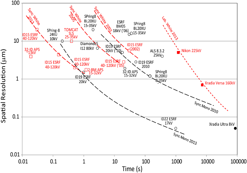
Plot showing the historical development of fast X-ray tomography. In many cases the spatial resolution is not cited and an estimated resolution twice the pixel size has been used. Open symbols denote synchrotron sources, while filled ones represent laboratory sources, red squares denote white beam and black circles monochromatic beam scanners. 26,31–42 The database on which this figure is based can be added to and is available in Ref. 43
Long timescale events (days/months): As illustrated by Fig. 1, laboratory sources are typically two orders of magnitude slower than synchrotron sources, but since they are competitive on resolution (see ‘Very high resolution imaging’ section), they are well suited to following structural changes that occur over periods of days or months. Examples range from the degradation of rechargeable batteries during their operating life 44 to the metamorphosis of butterflies. 45 For quantitative work it is important to remember that the accuracy is significantly influenced by the spatial stability of the X-ray focal spot 46,47 and that a stable position can take up to 2 hours to develop in certain circumstances. Rockett employed a UHV LaB6 source to circumvent stability issues associated with tungsten sources 48 specifically for long timescale quantitative studies. Such time varying effects need to be accounted for when quantitatively correlating or comparing images over extended timescales (see ‘Quantifying time lapse CT’ section).
Short timescales (minutes): There are numerous potential applications for imaging at the seconds-to-minutes timescale, for example Babin et al. 35 applied fast tomography to study the evolution of pores during bread making and showed that a gas cell structure first develops during fermentation. Afterwards, coalescence rapidly prevails leading to a heterogeneous structure. In a similar study Mokso et al. 32 have studied the dynamics of foam on beer. Pyzalla et al. 49 have coupled in situ fast imaging (one tomographic scan per 2 min) with in situ diffraction to study the creep deformation of copper samples. Imaging gave access to the evolution of the size of the cavities while diffraction was used to assess crystallographic texture, changes in domain size, dislocation density, and internal stresses. Vagnon et al. 50 employed fast imaging (1 min per scan) to study the deformation of steel powders during sintering.
This timescale is also ideal for following many damage accumulation processes, for instance to identify damage events in real time during the tensile testing of model metal matrix composites (spherical ceramic particles embedded in aluminium) coupled to acoustic emission measurements. 51 Here the deformation speed was set to a very low value (10−5 s−1) to prevent motion blurring of the reconstruction during the acquisition time (40 s). In this slow strain case it was found that continuous acquisition gave the same results, both in terms of imaging and acoustic emission acquisition, as interrupted straining. The same conclusions were drawn by Suery 52 for the ductile fracture of dual phase steels.
Second timescales: An extensive body of work has exploited fast imaging on the seconds timescale to study the coarsening, melting, solidification, and remelting of semi-solid metals. 34,36,37,53–55 For example special thermomechanical rigs have enabled the study of hot tearing, e.g. Terzi et al. 56 and Puncreobutr, Lee et al. 55 , which is important for solidification shrinkage during casting. It occurs during the final stages of metal solidification when the solid fraction becomes high, so that liquid is present only as a thin film when the liquid flow necessary to prevent tearing cannot occur. Direct observations of the evolution of hot tearing (Fig. 2a ) can be correlated with the measurement of the local strain field by digital volume correlation (Fig. 2b ) between successive images in the sequence and complemented by quantitative measurements of the void volume change (See Fig. 2c ). 55 Such in situ work has also shown that the results (e.g. the variation in the measured specific surface) obtained when characterising coarsening using a standard ex situ quenching and sectioning procedure are very different to what is observed under real time in situ continuous observation of the semi-solid microstructure. This is because significant changes in microstructure occur during quenching so that conclusions drawn based on observation of samples at room temperature can be misleading. 36
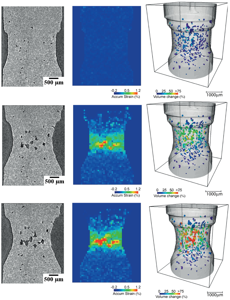
Fast imaging acquired during a high temperature tensile test of a semi-solid aluminium alloy. In this example, fast imaging is combined with digital volume correlation and image processing bringing new insights. 55 a A virtual section during the hot tearing of partially solidified metal, b the local variation in strain determined by digital volume correlation and c the volume change of the voids between steps, which shows the internal growth of the voids in the localised deformation region
Recently Deville et al. 57 have studied the solidification of ice crystals in a ceramic aqueous slurry in a process called freeze casting to produce lamellar porous ceramics with tomograms acquired in 1 second and a voxel size in the reconstruction of 1·7 μm. This can provide valuable information from a materials design viewpoint because of the scope for microstructural tailoring via control of the solidification conditions. 58
In this frame rate regime most of the work to date has been undertaken at synchrotron sources because of the greater flux. Nevertheless, recent advances in liquid metal lab sources promise to achieve nearly 10× the brilliance of standard X-ray tubes (achieving up to 300 projections per second 59 ), which may open up this area to laboratory imaging.
Sub-second timescales: Synchrotron sources can now acquire as many as 270 000 frames per second for radiography with tomographic frame rates moving towards tens per second (Fig. 1). The development of a special ultra-fast laboratory based X-ray scanner capable of acquiring one or two tomographic slices (i.e. not a full 3D tomogram) in one thousandth of a second has also been reported. 60–62 For this type of ultra-fast device, an electron beam is scanned very rapidly across a target to form a moving X-ray source used to illuminate a fixed sample in front of a fixed circular line of detectors (see Fig. 3a ). If the acquisition is synchronised with the scanning, it is possible to reconstruct tomography slices. In the device demonstrated in Ref. 60, the electron beam is scanned on a linear target. Acquisition is only partial and iterative algebraic reconstruction techniques (ART) are used for the reconstruction. The final image suffers from standard ‘partial angular view’ artefacts but the acquisition of single slices is nevertheless operated at a 1 kHz frequency. In Ref. 61, the images are of better quality as the acquisition arrangement is able to span 360°. The acquisition is again ultrafast, allowing the authors to study bubbles in a liquid for an air–water flow in a vertical pipe. In a new example, kindly provided for the present review, an acquisition speed of 2·5 kHz is reported while the system is potentially able to operate at 8 kHz (see Fig. 3b ). In fact a similar method was developed as long ago as the 1990s to undertake fast medical imaging 63 and a 3D scanner for airport luggage has just been commercialised. 64 In this case, up to 480 frames per second are collected with over 700 projection angles and a voxel size of 1 mm for an 800-mm inspection circle. All these lab systems have the advantage that the illumination moves rather than the sample, since the need to rotate the sample can limit the tomographic acquisition speed 32 or disturb the process being monitored.
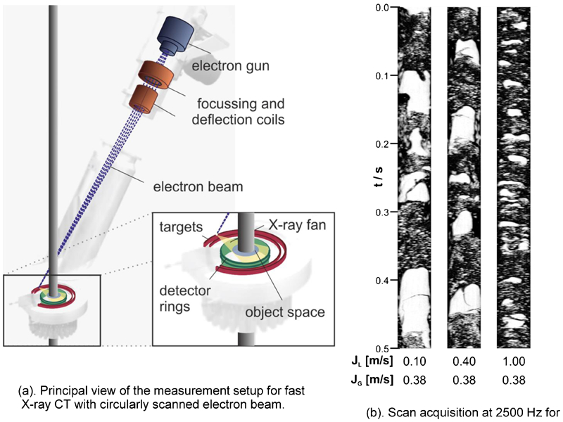
a Ultrafast electron beam X-ray CT system with two tomography planes and b example of imaged water–air two-phase flow. The flow has been imaged at 2500 fps, while the system is capable of a maximum frame rate of 8000 fps. The images show axial cuts through the three-dimensional data sets, where the vertical axis is time (adapted from Ref. 65)
Very high resolution imaging
Until recently micron resolution represented the state of the art. Sub-micron (nano) tomography is now available using both synchrotron and laboratory sources, although at markedly different acquisition rates (see Fig. 1). For nanotomography, optical elements are often used to focus the beam to a sub-micron point source from which the sample is illuminated as shown in Fig. 4.

Lens based systems, often called X-ray microscopes, can achieve sub-micron resolution; a Fresnel Zone Plate system, b Kirkpatrick–Baez (K–B) optics system, c Bragg multiplier system, d compound refractive imaging system (adapted from Ref. 66)
The majority of nanotomography experiments to date have either exploited: 66
Fresnel zone plates (FZPs)
Kirkpatrick–Baez (K–B) optics
Scanning electron microscope (SEM) beams.
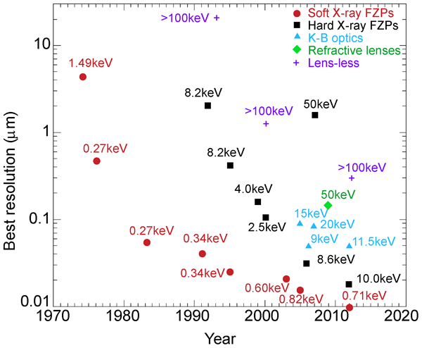
Fresnel zone plates: FZPs have been employed for high resolution imaging for many years. 67 As illustrated in Fig. 4, for soft X-rays (0·25–1·8 keV), extremely small focal spots can be produced. 68 Chao et al. 69 have used an overlay nanofabrication technique to make a composite FZP comprising two coarser complementary FZPs aligned to within 2 nm to give an outer zone width of 15 nm achieving a spatial resolution of around 12 nm at 0·815 keV at the Advanced Light Source (ALS), Berkeley. These energies are well suited to biological applications with the K and L edges of many elements including C, N, O, Fe and Al lying in this range. At a magnification of 2500, the field of view was only 10 μm. This in itself is not a serious limitation because at such low energies the method is limited to very thin samples anyway, for all but the lightest elements.
With increasingly hard X-rays the difficulty of making FZPs increases. Working in the 8–11 keV energy range opens up the edges of Cu, Zn, Ga, Ge, As, Ta, W, etc., appropriate to the semiconductor industry. Yin et al. 70 used 890-nm thick gold FZPs to image defects in W plugs at 60 nm resolution. These plugs interconnect the different layers of an integrated circuit and ‘keyhole’ defects formed during the electroplating process can cause the breakdown of the circuit. Fresnel zone plates begin to become impractical much above 10 keV though recent advances have seen 30 nm microscopes operate in the 3–30 kV range 71 with stacked FZPs being used right up to 50 keV. 72 Recently, commercial laboratory systems with sub-50 nm resolution have become available based on FZPs using Cu anode (8 keV) X-rays. 73
In view of the fact that it can take as long as a few minutes to acquire each very high resolution image, such tomographic datasets generally comprise only 50–200 radiographs. As the filtered back-projection reconstruction method does not perform well with such coarse angular spacing, algebraic reconstruction techniques (ART) are typically used (see ‘Novel reconstruction strategies’ section). Given that the exposure time is inversely proportional to the fourth power of the spatial resolution, and noting that their 30-nm FZP system takes minutes to acquire a single image, Yun et al. 74 suggest that X-ray tomography at resolutions significantly better than 30 nm is likely to be confined to synchrotron sources unless new lab. X-ray sources with greater brightness can be developed.
Kirkpatrick–Baez mirrors: FZPs become increasingly difficult to manufacture for X-rays above 8 keV. This has led to a number of harder X-ray microscopes based on K–B optics (see Fig. 4) including a zoom microscope capable of 90 nm resolution working at 20·5 keV using K–B mirrors 75 and a 50-nm microscope operating at 9 keV. 76 Harder X-rays are particularly well suited to the study of metals and matrix composites. Requena et al. used 17·5 keV for Al-based systems and 29 keV for Ti systems 77 at around 100 nm.
Electron microscope optics: Horn and Waltinger 78 were perhaps the first to realise that a SEM could be used for X-ray projection microscopy exploiting the highly focussed spot formed by the electron beam. With the arrival of field emission gun sources and improvements in detector technology, the method can come close to the capability of the high performance FZP X-ray microscopes, but at much more modest investment and greater accessibility. The spatial resolution and X-ray flux is dependent upon the choice of target (e.g. Au, Ag, Ta and Ti). The target determines the interaction volume, as well as the X-ray generating efficiency (increases with atomic number). By choosing targets such as Ag (or Ti) it is possible to obtain essentially monochromatic X-rays exploiting the 2·9 keV L α (or 4·5 keV Kα ) characteristic line. The thinner the target foil (<1 μm) the smaller the electron interaction volume and hence the effective source size. Strong phase contrast has been observed in images collected in this way 79 and a resolution better than 60 nm has been reported. 80 Burnett et al. 81 have combined non-destructive in-SEM X-ray tomography with destructive serial section FIB tomography to provide both time and high spatial resolution grain boundary information to study intergranular corrosion in Al alloys, coining the term ‘correlative tomography’. This combination of 3D imaging modes has considerable potential either to bridge scales or to provide complementary information.
Figure 5 summarises the resolution achieved using all these systems in the last five decades.
Nanotomography is beginning to have a very significant impact on materials science quantifying both materials fabrication and degradation processes. It helps quantify void nucleation and growth, 99 porosity and pore connectivity, 100,101 metal 77,102 (Fig. 6) and polymer 103 composite microstructures, fuel cells, 104–108 multiphase alloys, 109,110 self-healing materials, 111 and corrosion. 112 In the context of nanotomography the field of view is usually around 1000× the spatial resolution, which means that nanotomography is often synonymous with very small samples (see ‘Local tomography and laminography’ section), presenting both statistical sampling and engineering relevance issues, see ‘Caveats and cautions’ section.
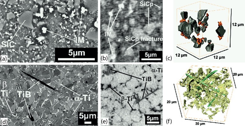
(Top) 2124 Al/25% SiC particle composite and (bottom) Ti64/5% TiB whisker metal matrix composites. Compared to back scatter electron images taken in the scanning electron microscope (SEM) (left), nanotomography images (centre) are of low resolution (100 nm) despite being at the current limits of X-ray tomography, however they do allow the 3D analysis of the spatial relationships (right) between the Fe–Cu intermetallics (orange) and the SiC reinforcement (grey), and the TiB needles (green) and irregularly shaped β grains (yellow) for the Al/SiC and Ti/TiB composites, respectively, 77 not so apparent from the 2D SEM images
Crystal grain imaging
In crystalline solids, the microstructure is often of key importance, influencing a wide range of material properties, including strength, toughness and corrosion resistance. For that reason, understanding and controlling the structure and evolution of grain boundaries is one of the central tasks of materials science today. This has led to the rapid emergence of electron back scattered diffraction (EBSD) analysis, providing detailed 2D maps of surface grain orientation.
While conventional absorption contrast cannot delineate crystal grains, new synchrotron X-ray techniques have recently opened the way to the non-destructive 3D imaging of grain structure. A number of methods have been developed, most notably one termed 3DXRD at the European Synchrotron radiation facility (ESRF), in collaboration with the Risø National Lab 113 and another at the Applied Photon Source (APS). 114
In the former a small, usually letter-box shaped, monochromatic beam is sent through a sample and, as in absorption tomography, the sample is rotated around an axis perpendicular to the beam. Each irradiated grain diffracts part of the incident beam. These diffracted spots are recorded by an appropriate detector. The experiment is repeated at three increasing distances between the sample and the detector so as to geometrically backtrack each spot to provide the position, shape and orientation of every diffracting grain. Such instruments have been used for mapping grains, 115–117 for studying lattice rotation during plastic deformation, 118,119 phase changes, 120 the nanostructure of materials 121 and for analysing recrystallization 122–131 as shown in Fig. 7. 132 In a variant, only a far field detector is used so that rather than doing real space imaging, only the centre of mass positions, relative volumes, mean orientations and full stress tensors for each grain within the illuminated volume is monitored. This was first achieved for a rather limited number of grains. 133–135 Recent progress has made possible a mapping of the stress field in a representative volume within the bulk of a polycrystalline sample using the individual grains as probes. 136–139
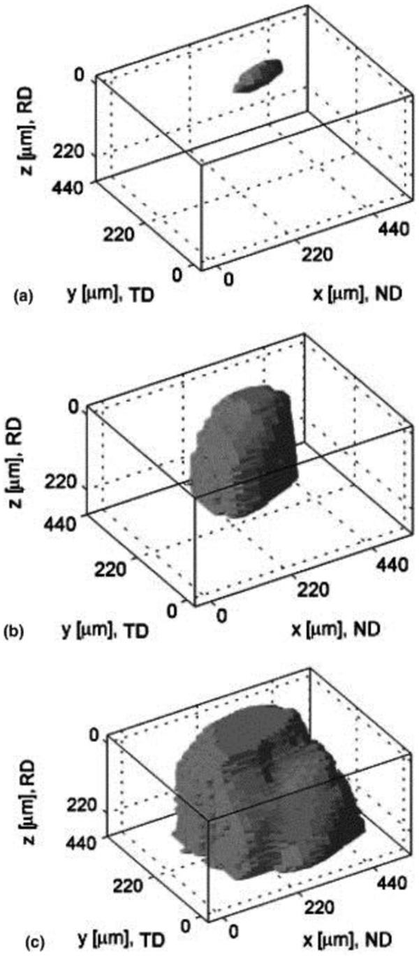
Illustration of the analysis of the shape and size of grains during recrystallisation using the capabilities of the 3DXRD method. The figure shows 3D maps of a growing grain in deformed Al. Three of the 73 recorded pictures are shown. a Picture 1, b picture 39 and c picture 59. In the coordinate system given, x-axis coincides with the normal direction (ND) (spatial resolution is 22 μm), the y-axis coincides with the transverse direction (TD) (spatial resolution is 4·3 μm) and the z-axis coincides with the Rolling Direction (RD) (spatial resolution of 6 μm) (adapted from Ref. 132)
In the latter a second technique used at the APS synchrotron, 140 a flat beam irradiates a slice of the sample and the diffraction pattern acquired at several distances. It involves a different approach in terms of reconstruction named forward modelling reconstruction (FMR). In this approach, the experiment is modelled in the computer. The irradiated sample plane is meshed with equilateral triangles and, in each triangle, a fundamental zone of crystal orientations is ‘searched’ so as to generate Bragg scattering that optimally overlaps that seen in the measurement. This procedure is computer intensive but gives robust results including in the case of deformed grains, 140–144 for studying lattice rotation during plastic deformation 118,119 and for mapping local strains. 145 Figure 8 shows a slice reconstructed at different strain levels using this method.
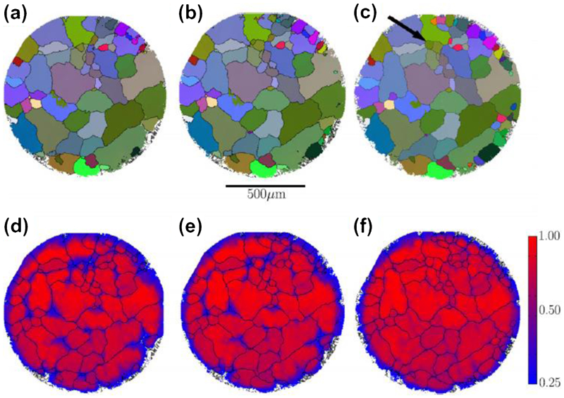
Illustration of the analysis of the shape and size of grains during annealing using the capabilities of the forward reconstruction modelling method. Grain maps for high purity aluminium (maps of the central layer of the measured volume) are shown. a–c show orientation maps in the initial, ∼50°C and ∼70°C anneal states, respectively. Each mesh triangle, or voxel, is coloured by mapping orientation components (Rodrigues vector representation) to the red-green-blue (RGB) colour space. Black lines are drawn between adjacent triangles that have mis-orientations>2°. d–f show maps of the confidence metric, corresponding to the orientation maps in a–c with the same black lines. The arrow in c indicates a nucleated grain 146
A third variant capable of providing grain maps is called DCT. 147–150 The set-up is rather similar to the one used for absorption or phase contrast tomography (PCT), the main difference being that a standard wide field imaging detector is used to acquire both the X-rays transmitted through the sample, but also those diffracted to wide angle by the grains currently satisfying the Bragg condition for a given angular rotation. Just as for absorption tomography, the sample is rotated around a vertical axis parallel to the detector. The rotation is achieved in very small increments to capture all the Bragg conditions. During a 360° rotation in 0·1° increments, each grain diffracts for about 10 angular positions. At these positions, the contribution of the grain falls in the direct image leaving a dark region because the X-rays are diffracted away and a corresponding wide field bright spot. From all the dark and bright spots the shape of each grain from this small number of shades can be reconstructed. The analysis of Friedel pairs of these diffraction spots allows one to determine the crystallographic orientation of the grains in the sample. 149,151 This method has been used to study intergranular corrosion, 152 the structure of snow, 153 of deformation, 154 and of fatigue cracking in titanium alloys 155 (see also Fig. 9). The approach tends to be limited to relatively low strains because the diffracted spots gradually broaden with plasticity making it increasingly difficult to infer the grain shapes.
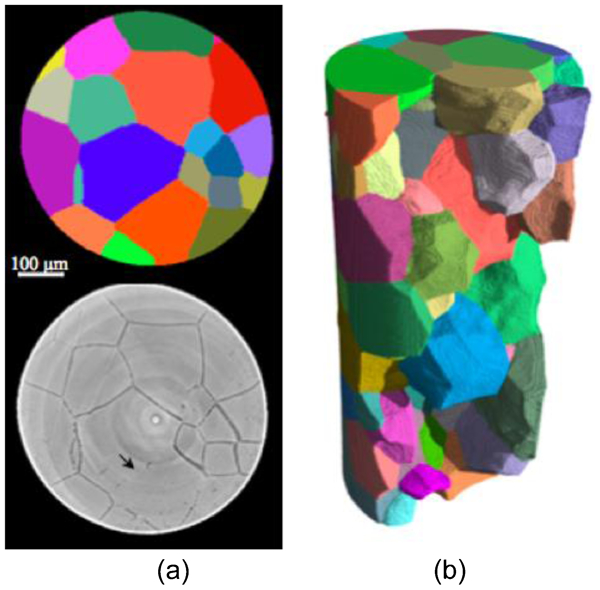
a Illustration of the capabilities of diffraction contrast tomography (DCT) to non-destructively produce a grain map of a polycrystal. Comparison of grain microstructure reconstruction of the same slice obtained from DCT and phase contrast tomography (PCT) in a beta Ti alloy. Layer-like precipitation of alpha Ti (hcp) reveals part of the grain boundaries in PCT. b 3D rendition of grain microstructure as reconstructed from DCT for the same sample 155
An alternative method is micro-beam Laue diffraction. It uses a narrow (20×20 μm say) polychromatic X-ray beam to illuminate a sampling volume within individual grains. The resulting single crystal Laue diffraction patterns consist of a number of Laue spots, which can be indexed to provide the grain orientation and elastic strain. 156 For thin slices, 2D mapping is relatively easy. For 3D scanning, vertical and horizontal fine wires of tungsten must be traversed just downstream of the sample in order to triangulate the location of the diffraction spots for each beam position making the process somewhat time consuming.
Novel reconstruction strategies
For materials science, most X-ray tomography datasets are collected by acquiring 2D projections as the object is rotated about an axis normal to the incoming beam using either a cone beam (normally lab.) or parallel beam (normally synchrotron) source. In the vast majority of cases these datasets are reconstructed to form an image using filtered back projection (FBP). Analysis suggests that qπ/2 projections are required where q is the number of detector pixels horizontally, 157 such that for a 2048-pixel detector around 3200 projections are recommended. This has developed from the original fan beam technique providing a single tomographic slice. The Feldkamp, Davis and Kress (FDK) 158 algorithm is a widely used cone beam FBP algorithm that can be regarded as a natural extension of the fan beam case. However, a circular cone beam scan is an incomplete data set for reconstructing the volume since Tuy's condition 159 is not satisfied, so that any reconstruction will be approximate except for the mid-plane slice. By contrast, parallel beam, helical and horizontal circle+vertical line scans all satisfy Tuy’s condition with medical CT systems employing helical scans. Consequently for cone beam imaging the approximation becomes increasingly inaccurate for large cone angles. As a result, the image quality degrades with blurring in the axial direction.
Beam hardening corrections: Artefacts can significantly affect quantification, for example ring artefacts and beam hardening (for polychromatic illumination) can lead to incorrect segmentation using simple thresholding strategies (Figs. 10 and 13). There are a number of experimental methods and procedures to reduce artefacts, 160 however special reconstruction algorithms can significantly reduce ring artefacts 161 and account for beam hardening. 162,163
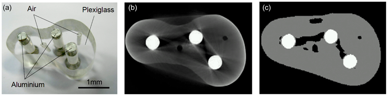
a ‘Barbapapa’ phantom comprising air, plexiglass and aluminium regions, b filtered back projection (FBP) image reconstructed from 300 projections acquired at 60 kV using a SkyScan 1172 computer tomography (CT) scanner showing significant beam hardening artefacts and c simple thresholding incorrectly segments the three phases in the phantom 163
Segmentation-oriented reconstruction: In cases where an object comprises a few homogeneous phases, and the primary intention is to distinguish these, it is not sensible to reconstruct the volume image using the full range of greyscales and then to apportion voxels in the image according to arbitrarily chosen threshold ranges. Rather it is more sensible to reconstruct the object with the prior knowledge that only a small number of grey levels are expected. Discrete tomography 164 considers the reconstruction of images from a small number of projections, where the set of pixel values is known to have only a few discrete values. It tends to deliver images that are more easily segmented than traditional FBP algorithms because the recovered image solutions are weighted towards a discrete number of more physically realistic grey scales, see Fig. 11 165 ‘Compressed sensing’ (see below) works in a similar fashion; it aims to represent many signals using only a few non-zero coefficients in a suitable basis. Clearly an image made up of a few intensity levels is simpler than one comprising the complete range of grey scales.
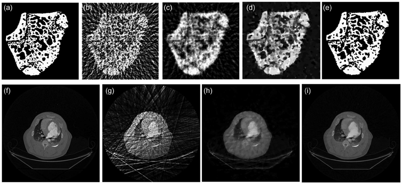
Top: a Phantom based on a rat bone and a comparison of reconstructions using 20 projections made by b filtered back projection (FBP) c Simultaneous Algebraic Reconstruction Technique (SART) d, Total Variation Minimization (TVMin) and e Discrete Algebraic Reconstruction Technique (DART); 165 Bottom: f FBP reconstruction using 642 projections of the body of a 47 kg swine acquired at 120 kV, g FBP with 20 projections, h compressed sensing (CS) using gradient image with 20 projections i prior image constrained compressed sensing method (PICCS) using 20 projections 166
Under-sampled imaging: There are many cases where 180° rotation is not possible (e.g. due to X-ray attenuation through environmental rig components, or by long path lengths through flat samples), or where too few projections are collected because the time to collect the recommended number is prohibitively long, or where the X-ray dose must be limited to safe levels. 167 In such under-sampled cases iterative algorithms can produce substantially better images than FBP methods. 168
For few-phase objects, discrete tomography and compressed sensing algorithms can be very effective at reconstructing images from low numbers of projections. Compressed sensing has shown that an NxN image can be accurately reconstructed using on the order of SlnN samples provided that there are only S significant pixels in the image. 166 Tomography images can be rendered more sparse by a number of means, for example by creating a new image in which the value of each pixel has been subtracted from its neighbours in x and y to create a ‘gradient pixel’. Chen et al. 166 have shown that when reconstructing a dynamic series it is possible to use a variant where the target image is subtracted at each time frame from the prior image (obtained by FBP using many projections) using a so-called prior image constrained compressed sensing method (PICCS) showing very promising results using an under-sampling of 32 (20 projections) as shown in Fig. 11. This method could find application when the number of projections needs to be restricted to capture short timescale events, or to reduce X-ray dose. Similarly the method is appropriate for sparse datasets comprising a few homogeneous phases that require segmentation.
Spatio-temporal reconstruction: Conventionally, a time sequence of tomograms is obtained by reconstructing each image independently. This frame-by-frame approach fails to exploit the inherent correlations along the time axis associated with measuring a real evolving object. Ideally, one should treat all the data from an imaging sequence as a whole, rather than as a collection of individual time frames. Clearly to reconstruct the whole sequence in one go would be a significant computational challenge, however there are significant benefits when the data is noisy or under-sampled. This challenge has started to be tackled in neutron CT 169 where the flux is characteristically lower such that only a few noisy projections are often collected, but the technique is equally promising, if computationally challenging, for X-ray CT.
Possible future directions: By reducing the signal required to create a satisfactory image, iterative imaging promises to significantly increase the rate at which 3D images can be obtained, benefitting fast imaging (‘Improvement in temporal resolution’ section), lowering exposure levels and widening the range of subjects that can be followed by time lapse CT. Further, iterative imaging can deal with blurring artefacts caused by motion. 170 One area that has not been explored significantly at present is metric-focussed reconstruction. For example if the ultimate aim is to quantify the pore morphology, then perhaps the reconstruction should be configured so as to identify iteratively the pore morphology present in the 3D image that is consistent with the projection data, rather than reconstruct the image without regard for the questions being posed and then extract the quantities by subsequent 3D analysis of the reconstructed images. This might also allow the iterative derivation of uncertainties in metrics associated with the image, e.g. cell connectivity in foams or the degree of crack face contact, whereas at present image reconstructions come with no associated error bars or morphological likelihood estimates.
It should also be noted that while iterative reconstruction techniques offer real advantages in a wide range of sub-optimal imaging reconstruction cases, their application is not straightforward and this has limited their uptake at the present time. In particular each iteration involves the forward-projection of the intermediate 3D image for comparison with the acquired projection data and subsequent iteration to minimise the difference between the two. However, commercial CT systems involve considerable calibration and correction of the detected data, and in some cases, proprietary optics. As Hsieh et al. 171 point out, model based iterative reconstruction requires an accurate forward model containing the optics, a noise model incorporating the detector sensitivity and calibration and an image model of the subject. Consequently this currently presents a significant barrier to the uptake of iterative methods such that most of the iterative algorithm development to date has been on simulated phantoms.
Chemical tomography
While conventional attenuation contrast tomography exhibits different levels of contrast according to the atomic number related contrast, it is not possible to distinguish chemical compositions with any certainty because many elemental compositions could give the same overall attenuation contrast. There are many cases in materials science where analysing the exact chemical composition in 3D (i.e. achieving chemical tomography) is of outmost importance to understand the mechanisms at play.
Like absorption, X-ray fluorescence is a well-known phenomenon. When irradiated by incident X-rays at a sufficient energy, electrons of inner shells of the constituent atoms can be ejected leading to chain rearrangements during which electrons from outer shells replace the ejected ones, in turn being replaced by other electrons, etc. X-rays of very well-defined energies are emitted during these rearrangements, and are known as the characteristic Kα , Kβ , etc. By scanning a pencil beam across a sample, and recording the number of photons emitted for these very particular values of energy, it is possible to record a sort of projection, the intensity being proportional to the local chemistry along the irradiated line. If such a projection is recorded for different angular positions of the sample, a tomographic reconstruction of the local chemical composition of the sample can be obtained. Such an experiment takes a very long time as the sample has to be scanned in one direction for each individual slice and each orientation. This has however been attempted using synchrotron radiation. 172,173
The same sort of experiment using a pencil beam has also been carried out coupled with a 2D detector to record the diffraction pattern. This was used to non-destructively reconstruct the map of the diffraction pattern in the acquired slice. This method is named diffraction tomography, 174,175 an earlier variant has been described using an energy dispersive detector. 176 It has been applied recently with a reasonable speed (acquisition of a slice in 20 min) for the study of structural change during high temperature modification of catalysts. 177 Alvarez-Murga et al. 178 reviewed some recent results on diffraction/scattering computed tomography. They showed that the method yields an enhancement in the detection of the weak signals coming from minor phases. In the same volume of the same journal, Stock et al. 179 report on a diffraction tomography study of an Al/SiC composite showing that the transmitted-intensity reconstruction agreed with that of higher resolution, absorption-contrast synchrotron microcomputed tomography. The reconstruction using the diffraction peak of aluminium (spotty rings) showed the presence of large grains, and the SiC reconstructions revealed the anticipated presence of two microstructural zones in the fibres. Korsunsky et al. used a similar approach to map residual strain after quenching a metallic sample. 180 Finally, in Basile et al. 172 both fluorescence and diffraction tomography have been carried out on the same sample.
All these methods require extremely long exposure times and are restricted today to long experiments at synchrotron sources. Previously, some level of elemental differentiation has been obtained using lab. sources by comparing multiple images collected using different X-ray energies 181,182 and using sudden changes in attenuation due to characteristic absorption edges as a function of energy to identify elements. Recent developments in energy sensitive area detectors 7 open up the possibility for this method to be applied quickly and efficiently in one imaging step using a polychromatic beam such as might arise from a laboratory source. We see a lot of potential in many applications for this new emerging technology. Nothing has been published so far in the field of engineering materials but Fig. 12 shows an example of such an energy sensitive image in the case of a USB memory stick.
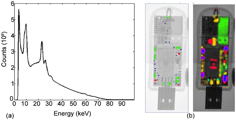
New possibilities are offered by energy sensitive area detectors as illustrated in this figure for a USB memory stick. Instead of a single image for one projection, a complete X-ray spectrum such as this shown in a is collected at each individual pixel. This allows many radiographs like that shown in b with regions showing specific absorption edges (red = tellurium, blue = barium and green = neodynium) to be reconstructed. b (right) Reconstructed X-ray fluorescence mapping of the dongle showing: bromine (green), tin (yellow), zirconium (turquoise), barium (blue) and silver (red) 7
Local tomography and laminography
The faithful reconstruction of a 3D image by FBP strictly requires the whole width of the object to remain within the field of view, and sufficiently illuminated, throughout the 180° rotation. 157 If this is not the case, there will be some missing data (some or all rows in the sinograms will be truncated) indicating that the standard FBP method is no longer strictly valid. This is known to give rise to artefacts in the reconstructions, most notably a centre-to-edge ‘glow’ artefact. 183
Given that CCD detectors usually have between 1000 and 4000 pixels across their width and the spatial resolution is a few pixels, this requirement to image the whole sample places a limit on the smallest feature observable to around a thousandth of the sample width. In many cases, for example, when imaging impact damage in thin plates, this means that the features of interest are too small to be observed by whole sample tomography. This problem can be countered to some extent by stitching together multiple images acquired side by side to create a large composite image as if a more pixelated detector were available 184 but this can be time consuming.
Local (or RoI) tomography refers to the acquisition of a tomographic scan under conditions where at least part of the sample is not projected onto the detector for at least some projections acquired during the scan. There are experimental approaches as well analytic and iterative reconstruction algorithms that can be implemented in such cases. One experimental approach to overcome this problem, termed here ‘zoom-in tomography’ is to combine low resolution information of the whole sample with the high resolution data within the RoI to produce a best estimate reconstruction. 185–187 This method has been demonstrated to be successful, 188 but can be difficult to apply in practice, both in terms of collecting the different magnification images and the subsequent accurate registration (both spatially and in terms of voxel values) of the low and high resolution projections. 189 Other analytic and iterative local tomography reconstruction methods are discussed in Ref. 190.
It has been shown that for a wide range of objects, the effect of truncation of the sinogram on feature detection in the RoI is negligible if (i) the truncated rows are extended by using an average value derived from the row that is extended and (ii) the number of projections (Qπ/2) is calculated not on the basis of the number of pixels on the camera, q, but on the number of pixels, Q, that would be required to scan the whole sample at the chosen pixel resolution. 189
There are also situations where the RoI reconstruction is straightforward without any correction because the missing region is isotropic in all directions, for example the X-ray transparent tubes used as a structural part of many in situ loading or environmental rigs, e.g. Ref. 191. In some cases, samples larger than the RoI are needed to ensure the images are representative of the bulk (either geometrically as for cellular solids, or in terms of stress state). Even if these materials are not completely isotropic, their effect on the projections may be effectively so. For example when loading cellular materials, uncorrected local tomography gives good reconstruction results, e.g. Ref. 192, because the effect of the foam cells outside the RoI is essentially the same in all projections.
There are many cases in materials research where the sample is extended in two dimensions (electronic devices, metal plates or composite sheets, etc.). For the same reason as those explained just above, high resolution tomography acquisition is not possible for 2D extended geometries. Laminography is an alternative to tomography in this case. Laminography, having been used rather early in medicine, 193 has been applied more recently in engineering science 194,195 using laboratory sources 194,195 and even nanoCT laboratory systems. 196 Traditionally laminography can be thought of as the collection of radiographs with the object being rotated about an axis normal to the plate but inclined to the incident beam, although in purpose built machines, the source and detector precess around the sample. More recently, laminography has also been implemented on synchrotron sources, allowing high resolution RoI images in the middle of very large sheet-like samples to be acquired focussing on specific regions near the centre of flat samples. This opens doors for the observation of damage processes during in situ loading of sheets. 197 Damage evolution ahead of a crack in composite laminates has been successfully observed using this technique in laminography experiments at similar resolutions as typically obtained by tomography. 198
Quantifying 3D images
Extracting quantitative parameters from 3D images requires appropriate image processing, segmentation and analysis. These three procedures have been applied extensively for the analysis of 2D images. Image processing is generally applied to ‘improve’ the image. It mainly involves grey level modification (equalisation, normalisation, brightness and contrast adjustment, etc.) and filtering (to remove noise or to subtract background) in the spatial or frequency domains. Segmentation is the procedure by which a continuous grey scale is apportioned to certain discrete groups, usually based solely on their grey levels. The aim is to define which regions of the image belong to the different phases present in the material. The grey level in the reconstruction being proportional to the local attenuation level corresponding to the appropriate phase, segmentation can often be made by simple thresholding but when the contrast between phases is faint, more sophisticated automated methods based on thresholds, clustering techniques or deformable models 199 can also be used. Image processing and segmentation in 3D are directly analogous to the same processes in 2D and so we will not focus on these two aspects in the present review except for some remarks at the end of this section.
Image analysis is probably the step where the most significant differences arise between 2D and 3D. It is devoted to the determination of meaningful measures of the constituent phases and their geometries, for example to quantify their number, fraction, size, distribution and surface topography. The development of many 3D tools has emerged as extensions of existing 2D methods. One easy way to exploit existing 2D approaches is to sequentially apply existing 2D tools to a volume slice by slice. Thresholding for phase fraction measurement, for example, can be done by pseudo 2D analysis, often with little impact on the results. By contrast, when the features in the microstructure have a complex morphology, such as corrosion cracks, coalesced cavities or cellular materials (foams, entangled materials, etc.), it is also important to use algorithms that are fully implemented in 3D.
Both global and local thresholding methods are used to quantify microstructure. In global thresholding, a single global greyscale value is selected to segment regions. 2D histogram methods where segmentation is done, (i) with respect to range of grey scale values or, (ii) with respect to the gradient of grey scale values are readily available in many commercial and non-commercial 3D processing software packages (e.g. Drishti, http://code.google.com/p/drishti-2/). In many cases these give good results, although because the phase fractions can often be linearly related to the choice of the threshold value chosen independent calibration of the threshold value may be necessary.
It was recognised early on, 200 in the context of bone mineral density measurement, that density variations and the poor resolving of thin cell walls could lead to spurious wall thickness measurements if global thresholding is used (Fig. 13 (top)). Measurements by global thresholding can be particularly sensitive to beam hardening if unaccounted for; increasing the apparent density towards the perimeter and decreasing it towards the centre causing particular problems for bone density measurement and other quantification procedures (Fig. 13 (bottom)). Rather than using global threshold values it has been found advantageous to select a local cut-off value using the frequency–distribution graph and a half-maximum height (HMH) measure. 201
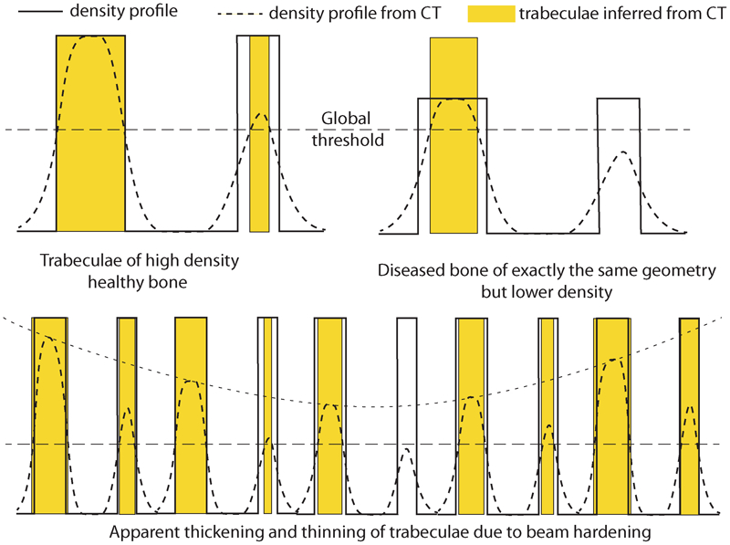
Diagrams of density profiles across trabeculae of various wall thicknesses and densities aid in understanding the problems that can occur in using uniform thresholds in the case of density variations (top) and beam hardening (bottom). The attenuation contrast profiles recorded by CT are shown dashed and reflect the spatial resolution of the method. The actual borders are given by the solid lines, the yellow regions, the borders inferred by CT using a global threshold (modified from Ref. 200)
Suitable algorithms have been developed both commercially and within the framework of open source packages. 202 The sections below discuss a range of archetypal 3D analysis problems performed on static 3D reconstruction of the microstructure. We also consider in this section examples where the authors have studied statistically the evolution of the microstructure from ex situ observation of several different samples. The quantification of changes in the microstructure over time during in situ experiments is further described in the ‘Quantifying time lapse CT’ and ‘Modelling based on X-ray tomography images’ sections.
Dimensional measurements
While the major focus of this review is on quantifying materials science microstructures, it is important to quantify the dimensional accuracy of parameters obtained from CT images, whether to ensure components lie within geometrical manufacturing tolerances, or to assess critical materials science metrics (e.g. the distribution of defect sizes across a casting). It should be borne in mind that for cone beam tomography, the Feldkamp, Davis, Kress reconstruction algorithm 158 is an approximation outside of the mid-plane (see ‘Novel reconstruction strategies’ section). The result is image quality degradation at high cone angles, often giving rise to blurring in the axial direction. As a result, features measured close to the mid-plane may be measured more accurately than those significantly above or below the plane perpendicular to the rotation axis, including the source.
As regards dimensional metrology, an international round robin was held recently drawing the following conclusions: 203
only a minority of expert users participating in the inter-comparison were able to perform length measurements with errors below the specification of their CT systems. However, the CT audit results indicate that length measurement errors in the order of 1/10th of the voxel size are achievable.
in the case of unidirectional length measurements, only 50% of the participants who quoted a maximum permissible error of length measurement EL,MPE were able to perform actual length measurement errors within their EL,MPE
in the case of bidirectional length measurements, only 33% of the participants who declared an EL,MPE were able to perform actual length measurement errors within their EL,MPE.
the participants had difficulties in evaluating measurement uncertainty appropriately: almost half quoted uncertainties that were smaller than their measurements would suggest and that traceability of dimensional measurements is still a major challenge in CT scanning, even for expert users.
a new testing method has been proposed for quantifying the structural resolution, based on an ‘Hourglass’ standard sample comprising two spheres in contact and measuring the apparent contact diameter, d: a smaller d value indicates a higher spatial resolution. A tetrahedral stack of equisized balls has been suggested as a standard sample elsewhere. 204
Inclusion/matrix morphologies
For bulk materials, the morphological character of second phases, inclusions or cavities are often of critical importance. In such simple cases the matrix fully embeds inclusions or voids, the parameters of which (size, elongation, surface, etc.) should be determined. This has been one of the major outputs of early tomography measurements on particulate composites 205,206 subsequently refined to quantify the local particle volume fraction 206,207 since clustering can have a detrimental effect on the fracture properties of composites. In Ref. 208 the authors have measured the size of clusters of reinforcing TiB2 particles and shown, using static imaging, that the size and number of clusters were reduced as the holding time at high temperature was increased. Toda et al. 209 have measured the growth of micropores in pure Al and Mg samples during high temperature exposure using a relatively high resolution (0·47 and 0·088 μm voxel sizes) clarifying that their growth is dominated by Ostwald ripening. Generally, it is better to quantify such populations from 3D images rather than 2D ones provided that precautions are taken regarding segmentation, resolution, etc., since it obviates the need for transforming a 2D size histogram into a 3D one. However, in all the cases listed above, where the shape of the inclusions is rather simple, 2D analysis coupled with stereology remains a cost-effective and useful tool. In our opinion, a systematic investigation of the bias induced by 2D imaging on the determination of 3D metrics is probably still required for specific morphologies. Conversely, tomography can also lead to quantification errors, for example the effect of insufficient resolution on the quantification of the nucleation stage of ductile damage has been highlighted in Ref. 210. The results at low resolution are strongly biased, due to the failure to detect a high number of small cavities while the largest cavities are faithfully recorded. Examples have also been given in the preceding section showing that bad segmentation or beam hardening effects can bias quantification.
When the shape of inclusions or voids becomes more complex, one can no longer rely on surface (2D) observation. Unreinforced aluminium alloys (AAs), for example contain a lot of so-called ‘intermetallic particles’; the size and morphology of these (including sphericity, local curvature radii and connectivity in cases of intermetallic content) has been quantified in Refs. 38 and 211–215. In cast metals (aluminium and magnesium), the complex shape of the initial morphology of the shrinkage pores is the key parameter determining their tensile 216 and fatigue properties. 217–220 In all these cases, the size of each cavity, as well as its sphericity, distance to the interface and projected surface perpendicular to the tensile direction, has been used for a better prediction of the fatigue crack initiation probability on each cavity. An example of such a quantification in Ref. 219 is shown in Fig. 14. This is also sometimes coupled with a Finite Element simulation of the stresses around each pore. 218,221
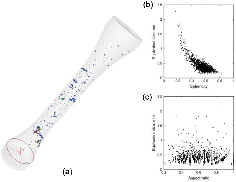
Illustration of the capabilities of X-ray tomography to quantify the morphology of pores in a metal. a Qualitative 3D view of defects detected by X-ray CT in a fatigue specimen in a cast aluminium alloy. 219 b and c Quantification performed using the 3D dataset (size, sphericity and aspect ratio)
Complex attributes such as the local orientation of anisotropic features (rod- or plate-like second phases in a matrix) have also been measured in metallic materials based on the so-called ‘grey level texture’ in the images. For this, it is necessary to calculate the gradient in the neighbourhood of each voxel. In Ref. 222 this value of the local orientation was needed to understand the structure of ‘Widmanstatten’ like microstructures in dual phase titanium alloy.
Cellular and highly porous morphologies
X-ray tomography is making a significant contribution in terms of 3D analysis for cellular materials: information that is not easy to capture using standard surface microscopy techniques. The major problem has been the availability of the software tools capable of performing the appropriate measurement on these connected systems. This is now largely solved, thanks to commercial and open source software suites (ImageJ, Avizo, VGStudiomax, Morpho+, Pore3D, Blob3D, Imorph). Some of the earliest studies were of trabecular bone morphology and were reported in 1989, 223 providing a measure of the three-dimensional connectivity in cancellous bone, local thresholding was used 200 to avoid spurious thickening or thinning of trabeculae either due to variations in mineral content or due to poor resolution of thin trabeculae. A rather complete investigation of many different morphological parameters (volume fraction spatial distribution, pore size and solid phase thickness, tortuosity, etc.) has been presented in Ref. 224, where a selection of different cellular ceramics exhibiting various morphologies (from honeycombs to stochastic foams) and pore size (from nanometres to millimetres) was imaged and subsequently quantified. In the case of closed cell foams, the same types of procedures as those used for inclusions in matrices described in ‘Inclusion/matrix morphologies’ section can be applied but in the case of interconnected pore networks, this analysis cannot be made as easily because in this case the notion of an inclusion vanishes and the sample often effectively contains a single large interconnected pore. For measuring the typical size of the pore in interconnected networks, specific 3D Image Analysis procedures based on sequential erosion/dilation operations applied to the binary images with structural elements of increasing size (this procedure is also named 3D granulometry) have been implemented. In Ref. 224 the implementation is performed in ImageJ, 202 an open source platform using the java language. Figure 15 shows (a) the materials investigated and (b) the cell size and wall thickness measured by such 3D granulometry operations. Other important parameters can be measured from these images like the specific surface and the tortuosity of the porous network (the ratio of the length of the path between two points in the porous phase over their distance in straight line).
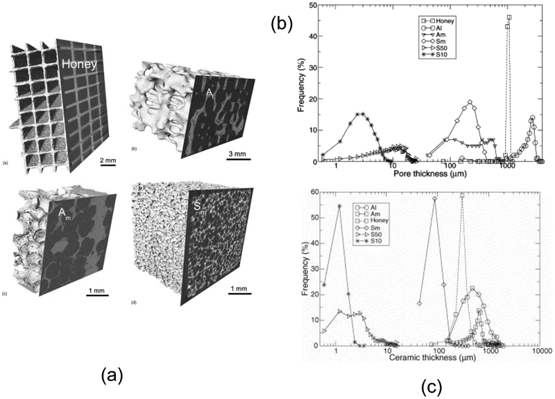
Quantification of the morphology of connected pores or solid phase in highly porous materials. The difficulty is that the phases are fully connected and special image processing methods like mathematical morphology granulometry have to be employed. a Qualitative 3D view of several cellular ceramics analysed in Ref. 224 and b the corresponding cell size and c wall thickness distribution
The paper by Brabant et al. 225 is a similar, more recent example where many porous samples were analysed and compared. The examples were also chosen to exhibit very different structures and scales: Euville limestone, pine wood, and two different grades of aluminium foam (20 and 10 pores per inch (PPI)). Rather than preserving the connectivity of the porous network and using granulometry, the pores were systematically separated in this latter paper using a watershed algorithm so that the fully connected network of pores was divided into subdomains. Different parameters could then be quantified: porosity, equivalent diameter and maximum opening distributions, orientation of the pores etc. This separation procedure also facilitates a simplified representation of the skeleton of the pore or of the solid phase. This is useful input for the modelling of transport properties and is available as an output from analysis software (imporh, avizo, Morpho+). After separation of the network into different pores, the pore throats can also be analysed (i.e. measured and used for the modelling of transport properties such as permeability). This has been achieved in Refs. 226–229 and is shown in Fig. 16.
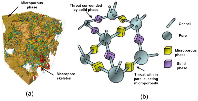
The description of a complex pore network can be simplified by the creation of a geometrical graph composed of nodes and tunnels. The specific dimensions of these simple elements have to be measured from the images. The figure shows as an example the transcription of a a porous network into b a network graph in a carbonate reservoir rock 226,228
Others have focussed on the pore size distribution. 230–233 In Ref. 234 this distribution was measured over several length scales using a suite of 3D imaging methods (X-ray CT, focussed ion beam serial sectioning, electron tomography) and is compared with Mercury intrusion measurements. Wall thickness measurement can also be achieved using 3D images. Foam strut thickness has been measured in Refs. 100 and 235. In Ref. 236 porous Ti alloys were analysed morphologically using interface shape and interface normal distributions and in Ref. 232 circularity was also measured.
It should always be borne in mind that most of these measurements are performed using approximations calculated using discretised (voxelised) images. This discretised nature can have a strong influence on the results, especially in terms of surface length and surface area, these parameters being overestimated for smooth objects (e.g. spheres).
Finally, it should also be remembered that some quantities are fractal such that their measured extent increases as the resolution of measurement increases; this is the classical ‘length of the coastline’ paradox. 237 An illustration of this effect is the finding that the measured surface area of porosity within a solid oxide fuel cell increased as the spatial resolution of the tomographic scan was increased. 238
Fibrous structures and other morphologies
Fibrous materials encompass polymer, ceramic or metals reinforced with elongated fibres, and also porous entanglement of fibres (like rock, glass or steel wools). In these materials, the size distribution is only rarely of interest 239 because the fibres often have a fixed diameter. The focus is more often the distribution of fibre orientations. 239,240 The structure can be rather complex in fibrous materials and was analysed in detail in Ref. 241 where 3D image analysis was carried out to skeletonise (simplified representation of the centrelines of the fibres) and construct a graph (determination of the coordinates of the nodes in the skeleton). Once such a graph is constructed it becomes rather easy to calculate parameters such as tortuosity and the distance between fibres. In Ref. 242 composites were studied but the fibres size and orientation were of no interest and the authors have rather focussed on porosity and its connectivity. Paper is a good example of entangled fibrous material where the knowledge of the microstructure helps to explain the macroscopic properties. Paper has been widely studied using X-ray tomography. For this type of material, (non-woven fibre mats) the interest is often on the distances between fibre to fibre contacts. This is a non-trivial measurement, fibre to fibre contact can be difficult to quantify.
In Refs. 243 and 244, auto-correlation functions were measured. This was used to analyse the isotropy in different directions for composite preforms and paper respectively. The auto-correlation functions are calculated from the correlation of a 2D image with a shifted version of itself of a given distance, d. This is generally done on binary images to analyse the spatial distribution of the white phase embedded in the black one. These functions are widely used in 2D image processing and their definition in 3D is directly analogous, by just changing the direction in which the sample is shifted. For instance, for a woven textile of carbon fibres, Badel 243 found that the correlation function of the fibres in the yarns measured in the plane transverse to the yarn remained very isotropic despite the progressive anisotropic deformation of the preform. This conclusion allowed the authors to significantly simplify the textile modelling strategy.
Density measurements
Davis et al. 160 point out ‘When Elliott and Dover first described X-ray microtomography in 1982, 245 they had one aim in mind: To devise a means of quantifying and mapping mineral concentration in biological hard tissue’. Further, they remind us that in many ways, today’s full-field scanners are not well suited for the quantification of the linear attenuation coefficient, which requires a well-defined source, the collection only of photons that travel in straight lines and a simple application of Beer’s law for attenuation. In trading discrimination for speed, today’s scanners collect scattered photons, often employ white radiation such that Beer’s Law is not obeyed (giving beam hardening) while CCD systems are prone to uneven pixel responses (ring artefacts) and charge bleeding. Indeed errors of up to 30% can be incurred due to beam hardening in estimating bone densities for 10 mm samples at 80 kV. 246 Consequently, it is very important for quantitative densitometry to make sure that the grey level fluctuation observed is only due to the change in density rather than compositional changes or imaging artefacts. Some artefacts, such as beam hardening can be corrected for (see Quantifying 3D images section), or avoided altogether by using a monochromatic beam, such as found on many synchrotron tomography beam lines. Uneven pixel responses can be normalised for, or removed by translating the detector during acquisition (so-called time delay integration 247 ).
The earliest quantitative voxel value measurements were aimed at measuring bone density 245,248 and carious teeth enamel 249 with demineralisation measured to better than 0·2 g cm−3. In materials science the technique has been used to measure the density variations across pressed and sintered powder metallurgy products, 250 the degradation of carbon–carbon composites 251 oxidised to different degrees over time, the reaction kinetics and morphological evolution mineral phases in cements. 252 In providing spatially and time resolved densitometric measurements the method provides much more information than simple conventional volume averaged densitometry measurements. By way of example, consider the loss of carbon during thermal degradation of nuclear graphite. 209,210 This graphite is extruded and medium textured, containing a mixture of coal–tar pitch binder and filler phase. The filler phase is composed of large needle coke particles (or grains), with an equivalent diameter in the range of 1 mm, and small crushed calcined particles, usually called ‘flour’, whose diameters are smaller than 300 μm. This kind of graphite was developed for use as the moderator in UK Magnox reactors. As illustrated in Fig. 17, tomography shows that the carbon oxidises preferentially, and not uniformly, in the binder regions made of pitch and small coke grains, rather than the filler carbon particles. 243,244,253,254 As the matrix phase loses weight disproportionately, this could have significant implications were structural integrity assessments based on average density change. Analytical models of the behaviour of the degraded graphite have been established based on the microstructural tomography data. 255
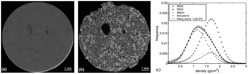
Comparison of virtual slices of a Pile Grade A nuclear graphite sample a before (WG0) and b after 30% weight loss (WG3) by thermal oxidation and c the histograms of the matrix and inclusions in their proportions corresponding to the best fit (77·5% matrix, 22·5% inclusions) 253 showing weight loss to be much more significant in the matrix phase
Caveats and cautions
It should be emphasised that 3D imaging should be the first choice option over 2D imaging only in special cases, since:
there are fewer instruments available,
the spatial resolution cannot compete with the highest resolution electron microscopes (see Fig. 6),
unlike the SEM it is not possible to examine regions of large objects at high resolution,
micro-CT necessarily leads to much larger datasets than for 2D imaging using optical or electron microscopes; this can leave all but the expert overwhelmed and struggling to reduce the volume of 3D data down to simple metrics,
except in special cases it provides no elemental identification,
few scanners can combine diffraction and imaging information, as is commonplace in electron microscopes, so provides little crystallographic information,
it is difficult to use anything other than FBP reconstruction codes on commercial scanners because of the lack of software available to the novice and the fact that proprietary information is needed to create the necessary forward model of the instrument,
the subsequent analysis typically takes at least an order of magnitude longer than it takes to acquire 3D data; consequently experiments should be embarked upon fully aware of the investment needed to analyse the results. Further results can be difficult to visualise and to interrogate,
while some basic analysis tools are available, either free or as part of commercial packages, analysis routines must generally be written by the user and so two users may obtain quite different results.
A continual problem with increased spatial resolution from an engineering point of view is the limitation this usually places on the size of the sample to be investigated (see ‘Very high resolution imaging’ and ‘Local tomography and laminography’ sections). Given that samples size is usually 1000× the spatial resolution or so, this can compromise the scientific or engineering merit of the observation; either from the perspective of a statistically representative volume point of view, or from a mechanically representative point of view. A good example of the former is the need for high resolution of geological cores, (which can be as long as 200 m), which for very fine microstructures such as those associated with shales, necessitates the imaging of millimetre sized volumes. A good example of the latter is the imaging of fatigue cracks in Ti/140 μm diameter SiC fibre composite. In this case micron resolution is required to quantify the crack opening displacement, but samples must contain a significant number of fibres for the crack growth to be representative of growth through the bulk from an engineering viewpoint. In this case image stitching strategies 184 were employed to allow a sample, 4 mm in size, to be viewed using a 1·4 μm pixel size. 256
Often, 3D imaging is best considered as part of a multi-scale imaging strategy. For example, micro-CT has been powerfully complemented by FIB serial sectioning and electron tomography to characterise the pore structure in catalysts across four orders of magnitude 257 as well as clays. 258 Similarly taken together, X-ray and serial sectioning electron tomography can provide both time dependent information and high resolution microstructural information. This has been termed ‘correlative tomography’ in Ref. 112 where non-destructive X-ray and destructive electron tomography were undertaken sequentially, both within a SEM. The non-destructive nature of X-ray tomography allowed the progress of corrosion of an AA 2024 to be followed over time at 100–200 nm resolution, but detailed examination of the localised corrosion (both chemical and crystallographic) was better performed by destructive serial sectioning and scanning electron microscopy (20 nm resolution).
In conclusion, X-ray CT should be restricted to situations where:
3D imaging brings superior information (e.g. the connectivity of 3D pore networks),
where the sample is very delicate (e.g. powder aggregates) and not amenable to 2D sectioning,
where the sample must be retained for archiving (e.g. museum artefacts),
where it must be observed in situ under conditions that make standard microscopy difficult (e.g. the microstructure of semi-solid metals) and finally,
where one needs to follow structural evolution in the bulk over time (e.g. damage accumulation under harsh environments).
In this regard as a non-destructive high spatial resolution method, X-ray imaging is particularly well suited to the quantification of structural evolution over time, as discussed in the following section.
Quantifying time lapse CT
In materials science and experimental mechanics, the evolution of structure can be very important during fabrication, throughout service life and as failure approaches. While observing the surface can be useful, in many cases structural changes occur hidden from view. Repeated (time lapse) 3D X-ray imaging allows one to follow the evolution of structure non-destructively in 3D giving rise to so-called 3D movies or 4D imaging. 259 While a pictorial understanding is often sufficient, in many cases a more quantitative view is required. Increasingly, this may be to evaluate the predictive capability of analytical or numerical models to describe behaviour.
It is often useful to quantify the structural changes that take place by static analysis of each 3D image in turn. However, it is also possible to quantify in 3D the distortions of the body through the 3D image sequence. By extension the spatial variation in displacement gives the local strain alongside any local rotations. There are a number of ways of extracting the displacement and hence strain field by comparing successive images. For 2D image sequences, particle tracking (PT) and digital image correlation (DIC) have become standard quantification tools. From surface images, it is only possible to retrieve the surface displacement/strain field. Recently these methods have been extended so that 3D movies of processes recorded in situ, can be used as inputs to deliver 3D strain or displacement fields. The capabilities of these methods are reviewed before going on to examine their use for the fracture mechanics assessment of crack propagation and the accumulation of other types of damage from time lapse image sequences.
Digital volume correlation (DVC)
Surface DIC is now well established, both for flat (2D) surfaces using one camera and curved (3D) surfaces using two, providing displacement vectors mapping an array of points from one image to the next. From these displacement vectors strain maps can then be inferred. Over time the technique has been successively improved in terms of displacement measurement accuracy (better than 0·05 of the pixel size) and calculation time. 260,261
Although DIC is now used extensively in the analysis of 2D optical microscope and SEM images (see Ref. 262 for a review of the topic), its extension to 3D tomograms (as reviewed by Bay 263 ) has only recently been gaining momentum despite the fact that the first example of 3D image correlation looking at bone was published many years ago. 264 This is probably because the availability of DVC software has been a problem and the first studies were made by direct collaboration between the developers of DVC codes and experimentalists. Recently commercial codes such as that produced by Lavision (www.lavision.de) have become available so this will surely accelerate the dissemination of the technique. Further, new correlation procedures such as that based on a global consideration of the entire sample rather than on sub-regions, 265,266 are being reported.
Just as for DIC, it has been shown 267 by quantifying the spatial resolution of DVC that the displacement uncertainty is related to the patch size by a -3/2 power law relation. The patch size itself has to be chosen as a compromise between the desire for high spatial resolution of displacement changes and the precision of the strain vectors. Provided the characteristic wavelength of the grey scale variation in the image is not too long, a typical lateral patch size of 8 or 16 pixels is generally a good compromise. One of the strengths of these methods is that the 3D displacement or strain field can be superimposed on top of the microstructure in order to relate heterogeneities in strain to the underlying microstructure as illustrated in Fig. 18.
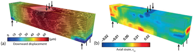
a The vertical-displacement field (in microns) determined by digital volume correlation (DVC) for a central region of interest (RoI, 0·44×2·69×0·56 mm) of a Scots pine sample (1·57×3·42×0·75 mm, tangential×longitudinal×radial) loaded in three point bending with the exterior loading points 2·51 mm apart on the underside (arrows). The 3D microstructure of the wood is overlaid. b The corresponding 3D axial strain field 268
Germaneau et al. 269 have compared strain measurement using X-ray CT and optical scanning tomography (OST) in transparent samples. They concluded that the displacement measurement uncertainty is around 0·037 voxels for OST and 0·049 voxels for X-ray CT. As the algorithms are complex, the computation time for full-field strain calculation can be rather large. This problem is addressed in Ref. 270 where strategies are applied to reduce this computation time. In this respect, graphical process unit (GPU) programming is likely to play a significant role in the future.
Digital volume correlation analysis has been undertaken on both laboratory or synchrotron tomography images of polymer foams, 192,265,271 the deformation of rock wool, 272 of wood, 268 of granular materials 273 and of geomaterials. 274,275 Besides materials deformation, the approach is able to monitor flow, for example the flow of powders during powder metallurgy processes. An example is given in Fig. 19 showing the movement of an Al powder during die compaction. Tracking the flow was aided by the inclusion of 20% of attenuating Sn marker particles. The higher levels of compaction achieved for a closed die as well as low compaction in the shear regions emanating from the corners of the moving punch are evident.
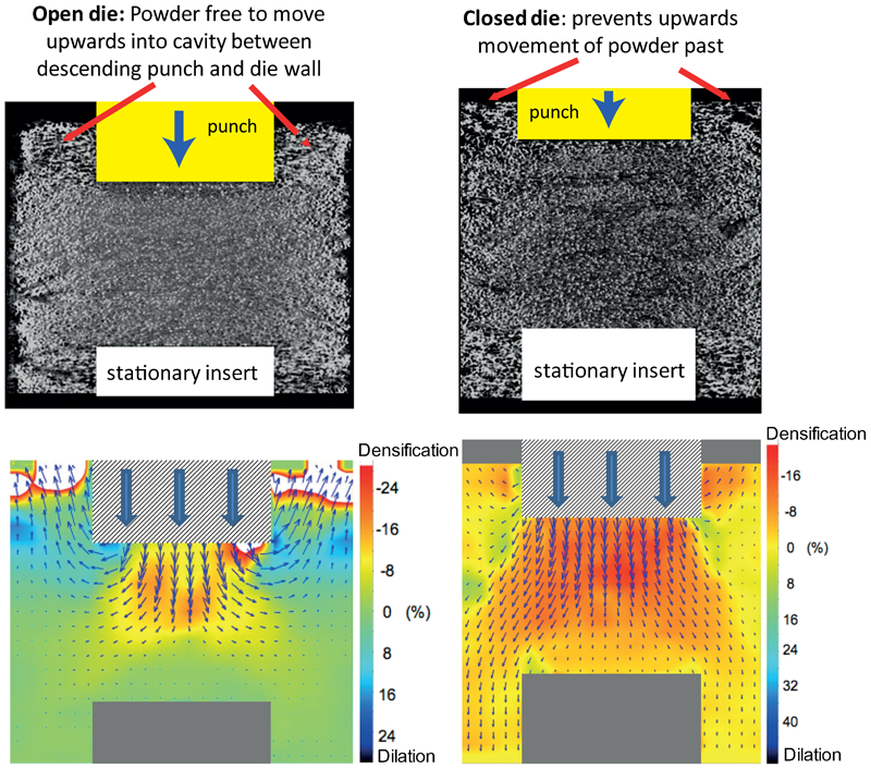
The displacements of an Al powder (grey) containing 20 vol.-% of Sn particles (white) during compaction by the downward movement (by 4 mm) of 10 mm dia. punch (left) for an open 20 mm dia. cylindrical die and (right) for a closed die. 276 The arrows indicate the displacements as the punch is moved downwards, while the colours represent the volumetric strains (densification negative)
Digital volume correlation is most appropriate for cases where the contrast varies continuously in space and grey levels, whereas feature-based tracking can be more appropriate in cases where the contrast is more discontinuous, for example isolated particles or precipitates in a homogeneous metal matrix. This is because in the latter case, the markers are too isolated to serve as ‘contrast support’ for a correlation measurement. To improve volume correlation, Bornert et al. 277 included a high proportion of fine Cu precipitates as markers when studying the deformation of AAs by DVC. A minimum volume fraction of 4% of these particles was necessary for precise DVC measurement.
Digital volume correlation is particularly well suited to dynamic studies as against pseudo-static tracking. It has been used to study the deformation of rocks 278,279 and the solidification of AAs. 56,280 The use of DVC in quantifying deformation around cracks is covered specifically in ‘Quantifying damage accumulation and crack growth’ section.
3D Particle Tracking (PT)
While image correlation focuses on correlating the grey level contrast across a patch with that in successive images, PT is more appropriate when images comprise discrete features against a homogeneous background, such as particles moving in a fluid or precipitates within a metallic alloy. For dynamic studies, PT can be carried out simply using just two projections (X-ray stereography), 281 but full CT provides much more spatially accurate information.
Tracking the centre of mass of particles or pores in a reconstructed tomographic scan at different states during the deformation of a material is a straightforward way of mapping the displacement and hence local strain field. The extension of standard PT techniques to 3D tomographic image sequences was implemented over 10 years ago. Initially standard video PT methods were extended to 3D. 282 Subsequently, a number of purpose designed algorithms have been proposed either focussed on observable features intrinsically present in the microstructure, 283 or added X-ray absorbing marker particles 284 (made of tungsten in their case). In both methods, the morphological characteristics of each microstructural feature, e.g. surface area, volume and centre of gravity, are measured precisely using techniques similar to these described in ‘Inclusion/matrix morphologies’ section. Strain is calculated from the physical displacement of each microstructural feature that is observed and recognised between two consecutive loading steps.
As for strain measurement, when a sufficient number of markers are dispersed in the 3D volume, the Delaunay tessellation algorithm, 285 which generates an aggregate of space-filling irregular tetrahedrons, is used to obtain the local strain distribution. The vertices of each simplex objectively define the four nearest neighbour marker microstructural features. Local strain is calculated in each tetrahedron, assuming a linear displacement field inside the tetrahedrons.
Numerous efforts have been made to improve the accuracy to a better level. A high resolution 3D surface construction algorithm, such as the marching cube algorithm, which gives a pentagonal faceted iso-intensity surface, is often used to improve accuracy to a sub-voxel level. The concept of cluster matching has also been applied by Kobayashi et al. 286 and shown to perform well in the presence of microstructural agglomeration. Nakazawa et al. 287 proposed a two-step tracking method that does not require the image registration step. Ando et al. 288 have recently published a version of the method applied to agglomerates of sand grains. They use the shape of each grain to map their kinematics, and detect local rotation and displacements (see Fig. 20). In this manner they found that the displacements progressively concentrate into localised bands (here 7–8 grains wide). The rotations were largely disorganised until the peak stress after which the rotations appear to be concentrated in a band somewhat wider than for the displacements. The width of the bands were found to vary with grain morphology, possibly as a result of grain interlocking for the more angularly shaped grains extending the rotations over a wider band. The use of PT for monitoring cracks is discussed in the next section.
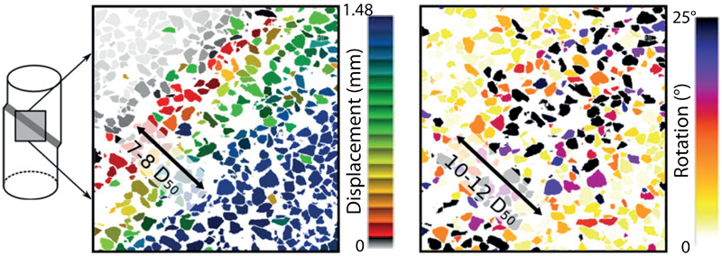
In contrast to digital volume correlation (DVC), discrete particle tracking (PT) does not treat the material as a continuum and so can identify individual particle rotations for example. Here approx. 1–2 mm grains of Hostun HN31 sand are subjected to a triaxial compression tests on dry material, performed at 100 kPa confining pressure 288
Quantifying damage accumulation and crack growth
As a non-destructive technique, X-ray CT can provide a very detailed picture of the evolution of damage through the life of a component. Furthermore the opportunity to host environmental stages means that damage can be followed in situ under a range of demanding conditions representative of those experienced in service. Consequently CT enables the quantification of a very wide range of failure mechanisms from transverse ply cracking in composites, to radiation induced cavitation in nuclear components at the tens of nanometre scale. Research focussed initially on ‘static’ measurements of crack length, 289 but advantage is increasingly being taken of the DVC or 3D PT techniques described above to quantify crack opening displacements.
In the move to develop materials that are both tough and strong, a range of crack-tip shielding mechanisms can be engineered into new materials, from crack bridging to self-healing. Such mechanisms mean that the crack-tip driving force experienced locally can no longer be related simply to the global parameters normally used to assess the propensity for crack growth (load, crack length and nominal crack-tip stress intensity factor). X-ray CT provides one way to both observe the activation of crack-tip shielding mechanisms and to quantify their efficacy.
Regarding the level of damage that can be detected, provided they cover a number of pixels, round pores are relatively easy to observe. Determining the presence of cracks tends to be more troublesome. This is because a closed crack is not visible to tomography. Often this need not be a problem if there is an opportunity to study the sample under load so that any cracks are held open. If analysed using DVC or PT, the displacement field around such a loaded crack can also reveal its presence even if the crack is invisible in the image. Further, the fact that a crack is a planar defect means that, in contrast to point defects, they can often be detected even when they are narrower than the pixel size. As discussed by Stock, 1 the narrowest crack opening that can be measured by tomography is a function of the pixel size and the contrast difference. Breunig et al. 290 suggest that for aluminium a crack as small as 10% of the pixel size can be measured using a 40 keV lab, system with an Ag target. For a 2000 pixel wide sample this would represent a change in contrast as small as 5×10⁻⁵ in a given projection. For polymer composites illuminated with X-rays from a 100 kV tungsten source, a sensitivity to cracks 20% of the pixel size has been quoted 291 improving to 5% if dye penetrant is used to enhance the contrast. However, these values appear rather optimistic under all but the most favourable conditions. In recent years considerable attention has been focussed on using propagation phase contrast 292 to enhance the detectability of cracks. 293,294 While this does aid crack detection, because of the Fresnel edge contrast, it can be more difficult to quantify the opening of the crack. 295 Wright et al. 103 report a crack sensitivity of 14% of a pixel for polymer composites with phase contrast.
Quantitative 3D fracture mechanics
In traditional fracture mechanics approaches there are a number of metrics used to determine the propensity for crack growth including; the elastic energy release rate, G, the stress intensity factor, K, the J integral, the crack-tip opening displacement (CTOD) and the crack-tip opening angle (CTOA) as well as the identification of key mechanisms such as closure that can modify that conditions local to the crack-tip and thereby slow or accelerate crack growth relative to that which would be expected solely in terms of the global parameters. X-ray microtomography can provide a quantitative measure of many of these. 296
Crack face closure: High resolution X-ray imaging can be used to determine when the faces of a crack close during fatigue crack cycling. So-called crack closure is an important mechanism in retarding fatigue crack growth. 297 It has been studied by CT as long ago as 1995 298 revealing how the topology of the fracture surface of Al–Li alloy determines the onset and extent of closure during unloading from the maximum load. In this case asperities hasten crack face contact during unloading prior to the ‘knee’ in the crack compliance curve. This ‘knee’ appeared to coincide with load bearing across a significant fraction of the crack faces. 298,299 Subsequent work 283 substantiates this showing that in many cases loss of crack face contact occurs gradually up to the maximum load rather than at a single definable opening level. For AA, Khor et al. 294 observed the crack surface topology, bifurcation and tip geometry using gallium to delineate the grain boundaries (which are usually invisible to CT) to understand the interaction of the crack with the grain structure. A number of crack closure studies have followed for Al–SiC 300 and Ti–SiC composites, 301 cast iron 302,303 and AAs. 304 It is important to remember that closure is believed to influence crack growth though the extent to which it shields the crack-tip from the full range of the stress intensity range. In many cases tomography suggests that the faces touch well before the conventional change in sample compliance during unloading normally associated with the onset of crack face contact. 305 This is not by itself confirmation that closure will affect crack growth since tomography cannot determine whether significant loads are borne across the faces.
Crack-tip opening displacement: As well as its importance in determining crack face contact from the point of view of closure mechanisms, the degree of opening and closing of the crack can be related directly to the crack-tip driving force. There have been a number of ways in which the crack opening displacement has been measured which fall predominantly into two groups; namely those who have measured the crack opening directly 301 as will later be explained in Fig. 23a and those who have used PT (Fig. 21) 306–308 or digital volume correlation (Fig. 22) 309 to study the crack displacements. Figure 21 shows as an example the fracture of an aluminium sample where a sharp fatigue crack was previously introduced. The tomographic images were recorded using fast tomography (20 s for acquiring a scan with a 1·6 μm voxel size) during a continuous tensile test and the fracture mechanics J integral parameter was thus determined.
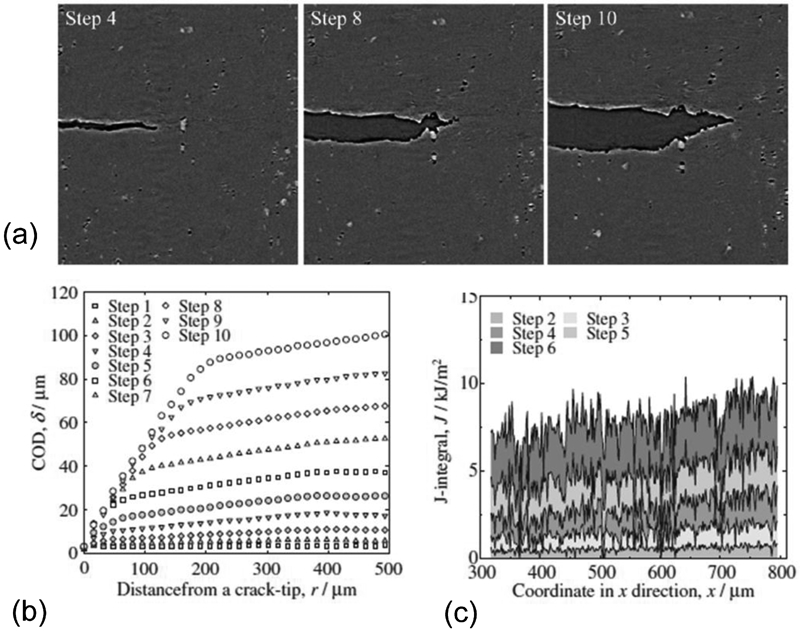
Particle tracking (PT) can be used to quantify some fracture mechanics parameters and their evolution during a fast in situ tensile fracture test. 310 a Virtual tomographic slices representing typical crack-tip morphology and its evolution at various steps to failure. The images are acquired using fast tomography during a continuous tensile test for a pre-cracked AA. b Crack opening displacement profiles averaged across the line of the crack obtained from tomograms such as in a and c Variations in the value of J along the crack front (x) for the first six steps, obtained by PT
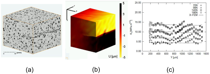
The figure shows the displacement inferred by digital volume correlation (DVC) analysis of the combining synchrotron X-ray computer tomography (CT) images. 309 a Tomogram of crack in nodular cast iron, b displacement field surrounding the crack at max load determined by DVC from images at minimum and maximum loading, by c comparing extended-FEM with the DVC displacement map can infer the variation in mode I stress intensity factor along the crack front after 45 000 cycles
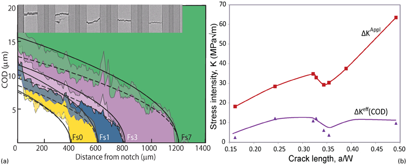
a Crack opening displacement (COD) measured near the mid-plane for a fatigue crack observed intermittently at K max (upper lines) and K min (lower lines) during fatigue crack growth in a Ti–35 vol.-% 140 μm diameter SiC fibre composite along with the best fit r 1/2 curves, b variation in crack-tip driving force with increasing crack length compared to that nominally applied (ΔK Appl) as inferred from the best fit r 1/2 curves for the COD data at K min and K max in a 256
Along similar lines, DVC analysis of the movement of graphite nodules in CT images of cast iron during crack opening have been coupled to the extended finite element method (X-FEM) 311,312 to quantify the local crack driving force along non straight cracks. 309 An example of this is shown in Fig. 22. This highlights the synergy between imaging experiments and state of the art numerical simulation. X-FEM is first shown to both improve the crack detection thanks to the enriched Finite Element basis used in the study. This approach has also led to the concept of X-DVC, which is based on a global approach to volume correlation (as opposed to standard local approaches where patterns are recognised one by one using the correlation of sub-volumes of the image). The finite element tools also have the advantage that they can be used directly to post-process the measured displacement field (including the singular components) to extract stress intensity factors along the crack front.
Either way, the change in the crack opening displacement (COD) during the loading cycle can be used to quantify the local crack-tip driving force. For the Ti/SiC data shown in Fig. 23a
, it was predicted that the COD would vary as √r depending on the effective stress intensity
313
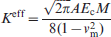
Stress intensity factor: the PT and DVC methods can be used to provide a measure of the total displacement/strain field around a fatigue crack.
256,314
This method was first used by Toda et al.
306
to derive the local mode I, II and III crack driving forces K
I, K
II, K
III from the local displacement vector u(x,y,z)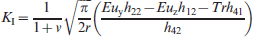
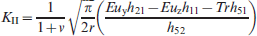

While a great deal of the work to date has been focussed on metals and alloys, CT analyses of crack propagation are becoming more widespread in other areas, particularly with respect to more complex structured materials including 2D and 3D composite systems, 103,291,316 self-healing systems 111,317 and crack propagation in natural materials, e.g. bone, 318–320 teeth, 321 wood, 268 as well as graphite, 322 which is an important structural material for the nuclear industry. Mostafavi et al. 323 found from surface DIC that unstable fracture is preceded by the sub-critical propagation of surface cracks having a scale similar to the microstructure. Using a chevron notch geometry to obtain straight cracks, the crack opening displacement was measured by DVC in 3D (see Fig. 24). The experimental values are consistent with the FE-predicted values and demonstrate the existence of a cohesive fracture process zone ahead of the crack-tip (Fig. 24b ). This suggests that simulations of the fracture process require a material model capable of showing local softening behaviour.
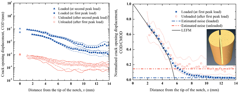
a Distribution of crack opening displacements (COD) along crack in a chevron notched graphite sample under loaded and unloaded conditions: the bounds show the minimum and maximum values of COD along the crack front. b Comparison between the average COD measured by digital volume correlation (DVC) from CT images normalised by the crack mouth opening displacement (CMOD at the free surface) and finite element simulation prediction after the first loading stage: average crack length is 5·7 mm and peak load is K max = 1·60 MPa√vm, 324 tomogram of sample shown inset
Crack growth, crack bridging and crack path
Extrinsic toughening mechanisms act to slow the rate of crack growth by shielding cracks from the nominally applied crack-tip stress field. Two important mechanisms are crack deflection and bridging. It is relatively easy to quantify the crack path and shape 325,326 as well as the crack growth rate by incremental CT imaging.
Crack growth rate: Marrow 327 measured the crack growth rate of short fatigue cracks initiating from graphite nodules in aus-tempered ductile iron by CT and found the crack growth rate to be very uneven with periods of fast growth rate, punctuated by periods when it is essentially arrested. Buffiere et al. 191,325 have looked at the morphology of cracks and correlated this to the crack growth rate of longer cracks as a function of fatigue cycling. To quantify the relationship between crack growth and grain orientation 328 or the nature of the grain boundaries 152 it has been necessary to exploit the grain mapping methods summarised in the ‘Crystal grain imaging’ section 152 or undertake post mortem electron back scattered analysis. 329 Birosca et al. 330,331 created three types of microstructure for dual phase titanium alloy, namely lamellar, duplex and a heterogeneous combination of the two. Of these, the lamellar microstructure displayed the fastest and the duplex microstructure, the slowest crack growth rate. Computer tomography showed that a columnar lamellar microstructure creates a relatively smooth crack front while a basket-weave type microstructure forces the crack-tip to undulate on the lath width scale. Vast differences in the extent of crack growth rate between the interior and surface have been revealed by CT for nuclear grade graphite such that without CT, fracture mechanics analysis would be totally misleading. 322 The relationship between microcracking in alumina and grain orientation has been examined though a combination of conventional CT to identify the microcracking and DCT to map the grain orientations. 332
Crack deflection and bridging: In many cases a key aspect in crack-tip shielding is the presence of bridging ligaments. While these can be imaged qualitatively in a straightforward manner, quantitative analysis is more difficult; Babout et al. 333 have developed algorithms that allow the tracking of the location and extent of the bridging ligaments as they neck down while the main crack progresses further downstream. Other works have focussed on crack deflection and crack bridging of both transgranular 328 and intergranular crack growth. 334
Many natural materials are extremely anisotropic giving rise to extensive crack deflection, e.g. wood, sea-shells, bone, enamel/dentin and elephant tusk. For example, for bone, three-dimensional imaging of cracks growing transverse to the length of the bone shows marked crack deflections and (out-of-plane) twists as it interacts with the underlying haversian structure. 335,336 This is a major source of toughening for cracks grown in this orientation. For cracks growing along the length of the bone, microcracks tend to form ahead of the crack along the lines of the haversian canals, which then give rise to crack bridging as they join the primary crack. The increased osteonal density in older bone leads to smaller and less frequent crack bridges and correlates with the marked reduction in the slope of the R curves with age. 319,337 This toughening mechanism is less effective than the crack deflection that arises when a crack grows transverse to the length of the bone.
Void/Damage evolution
There is an interest in the evolution of voids both in terms of their elimination during manufacturing of powder metallurgy components and their nucleation and growth in service leading up to failure. During manufacturing CT has been used to quantify the relationship between void size and morphology and densification and to understand the contribution of plastic flow, diffusion and other densification processes for metals, 338,339 ceramics 257,340 and even for ice. 341 During life, the growth rate of particular families of tension or creep cavities are of interest. Perhaps one of the first to quantify the evolution of damage during straining was Buffiere et al. 205 later followed in the studies in Refs. 206 and 342 who found that in low strength aluminium alloy–zirconia/silica particle composites, matrix voiding and particle matrix decohesion were the dominant mechanisms of damage accumulation whereas for stronger matrices, particle cracking was more common (see Fig. 25).
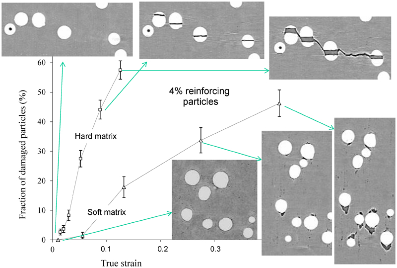
Quantifying the extent of particle cracking and particle/matrix decohesion in high strength and low matrix strength Al metal matrix composites containing 4% spherical ceramic particles. Tomography is needed because the damage of near surface particles in not representative of the bulk. Re-arranged from Ref. 206
The capability of 3D imaging to quantify separately the nucleation of new cavities, 343 their growth 344 and finally their coalescence 345 has also renewed the interest of the experimental study of ductile damage during tensile deformation at room and high temperature in engineering materials. 345–347 In a series of studies on ductile fracture of steels 348,349 and AAs, it has, for instance, been shown that rather than tediously trying to follow each cavity in the entire population (sometimes amounting to thousands of individuals cavities), cavity growth was much more easily quantified using the average diameter of the largest cavities in the population. Cavity growth has then been experimentally quantified with some confidence and this is currently being compared with the prediction of various cavity growth models.
A number of in situ and ex situ creep studies have also been carried out. For instance, copper was tested at 50% of the melting temperature indicating that growth of voids with radii of a few microns is determined by a viscous flow mechanism. 99 By following the evolution of individual voids it was concluded that void coalescence follows two stable growth regimes involving the impingement of neighbouring primary voids, followed by the coalescence of secondary voids before final rupture. 350 For Al+Al2O3 particle containing composite, there is a change in the damage mechanism with matrix delamination and matrix voiding occurring at high temperature (300°C) but particle fracture contributing at 200°C. 351 The pore volumes and number increase linearly with strain but exponentially with time such that the average pore size remains essentially constant.
In an investigation of the creep of a brass alloy (Cu–40Zn–2Pb), the evolution of the shape and size of creep cavities was followed as a function of time by synchrotron X-ray tomography 49 (Fig. 26). Traditional metallographic observations suggested that their shape ranges from almost spherical to a crack-like morphology for comparatively large cavities depending on the loading conditions. 352 Four types of cavity were identified by CT. 353 In the initial state, ellipsoidal cavities were dominant, but as creep progressed, while the total volume of all four types of cavities increased, the volume of spheres and rods grew far less rapidly than did ellipsoidal and complex shaped cavities. The predominance of ellipsoids and their total volume during primary and early stage of tertiary creep (a true secondary creep regime was not observed) suggests that surface diffusion around the cavity is rapid enough to maintain the shape of the growing cavity 354 at this stage. A rapid increase in the volume of the complex cavities was noted when tertiary stage creep became more pronounced.
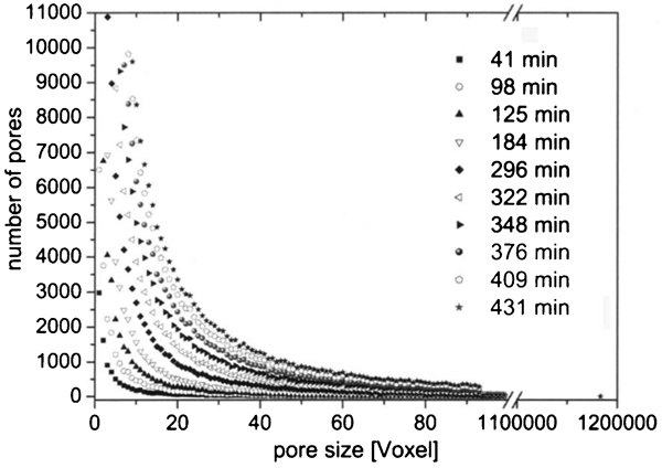
Quantification of the number and size of voids during creep for Brass (58 wt-% Cu; 40 wt-% Zn; 2 wt-% Pb) crept at 375°C under a load of 25 MPa 49
In this field, it is becoming clear that, allowing the observation of the interior of a sample without requiring a specific (and possibly biasing) preparation procedure, X-ray tomography is the best way to obtain reliable information on the evolution of cavities during loading (mechanical or thermal). This has enabled many, well established and widely used modelling theories in this field to be revisited. Some have been validated (e.g. the Huang model for damage growth during ductile fracture 344 ) and the weaknesses of some of the others highlighted (e.g. Brown and Embury criterion for void coalescence in ductile fracture 345 ).
This has to be applied with caution though, mainly because the resolution has to be high enough to allow the visualisation of all the cavities of interest many of which can be quite small.
Corrosion
X-ray tomography is finding increased application in the study of corrosion. 355–358 This is in part because gross measures of corrosion such as weight gain and electrochemical activity tell one little about the location and extent of localised corrosion, which can often be the biggest concern and often because small features at the surface belie extensive sub-surface corrosion. Localised corrosion rates can be many orders of magnitude greater than for general corrosion. CT is particularly useful for pitting corrosion or other cases where a small entrance hole conceals extensive sub-surface corrosion. In this section we will concentrate on example cases where quantitative tomography has been applied.
The grain boundary relationships are critical to controlling intergranular stress corrosion cracking, for example of stainless steel. Conventional CT is an excellent way of following the growth of SCC cracks over time, 356 but DCT provides a means of mapping the boundary orientations along the crack path. Through such a quantitative analysis it is possible to identify the nature of the grain boundaries that are resistant to SCC (see Fig. 27). King et al. 152,359 have shown that a range of grain boundaries have ‘special’ properties and may be involved in crack bridging during SCC, not just low coincidence site twin variant grain boundaries (Σ3). These include Σ1, Σ3, Σ9 and Σ11 boundaries with low hkl planes on either side.
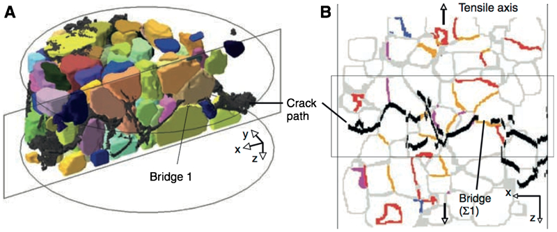
Combined use of diffraction contrast tomography (DCT) and computer tomography (CT) data to identify the nature of crack bridging grain boundary relationships during stress corrosion cracking of stainless steel. a Cracks obtained from CT data are shown in black, at the final step before sample failure, and compared with DCT data of 3D grain shapes. b 2D section of the grain boundaries identified by DCT (low angle Σ1 orange; Σ3 red; Σ9 blue; other boundaries Σ<29 purple) compared with the crack path (black) identified by CT 152
Corrosion is not always something to be avoided; there is now a serious focus on biodegradable Mg implants for medical applications. However, the degradation process needs careful control as magnesium corrosion creates H gas. If the local hydrogen saturation of blood and tissues are exceeded, hydrogen gas accumulates in tissue cavities. Witte et al. 360 have studied the use of coatings to slow corrosion to acceptable rates (see Fig. 28) using thresholding techniques to quantify the volume lost to corrosion.
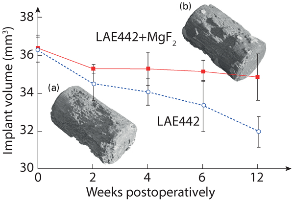
The implant volume of LAE442 and magnesium fluoride (MgF2)-coated Mg alloy LAE442 at different postoperative intervals. Results were obtained from computer tomography (CT) images. The morphology of in vivo corroded a magnesium alloy LAE442 and b magnesium fluoride-coated LAE442, 12 weeks postoperatively are shown inset. The dominant corrosion morphology was pitting corrosion (a and b) 360
Modelling based on X-ray tomography images
The use of tomographic images, both to set up geometrical models of materials and also to validate their performance in predicting structural changes is an emerging trend in materials science. We first describe briefly the available procedures to mesh the tomograms before giving an extensive review of the recent papers using this technique.
Mesh generation
It has been proposed in Ref. 361 to classify the different approaches for generating a mesh that is microstructurally faithful into three families:
Method 1: meshes using beam or shell elements,
Method 2: voxel based quadratic meshes,
Method 3: tetrahedral meshes filling a surface made of triangular elements
Figure 29 shows a visual sketch of this classification. It appears that the most popular method is the third type.
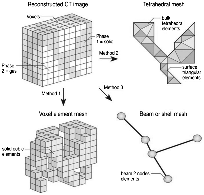
Visual sketch of the different methods available for meshing 3D images, adapted from Ref. 361
In all cases, one of the main issues is to capture sufficient geometrical detail to be faithful to the image based microstructure, while at the same time keeping the number of finite elements computationally tractable. Overmeshing is the main limitation of these methods as the images are sometimes so big that the number of elements exceeds the capacity of the standard commercial codes. Four methods have been investigated to overcome this issue: down sampling (or binning) explored, for instance, in Refs. 255 and 362, the use of a dedicated FE code as suggested by Roberts and Garboczi, 363 the parallelisation of standard FE codes such as paraFEM (www.parafem.org.uk), for example in Ref. 364 or in Madi et al. 365 and finally techniques based on the Fast Fourier Transform (FFT) initially developed by Moulinec and Suquet. 366–370 Figure 30 gives examples of several meshes published in the literature.
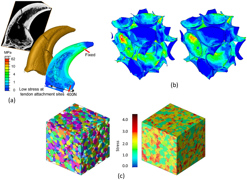
Examples of mesh geometries created from tomographic images; a tetrahedral mesh: contour map of Mises stress through the mid-section of a (repaired) velociraptor claw loaded at the tendon location and constrained at the tip; 371 b shell mesh: contour map of the Mises stress calculated with shell elements based on a tomogram of a steel hollow sphere structure (left); the result of the calculation is also compared with a mesh of the same tomogram with tetrahedral elements showing similar trends (right), adapted from Ref. 372; c Voxel mesh: Fast Fourier Transform (FFT) calculation of the elastic stress field (left). The mesh is generated from a numerical, two-phase digital material containing isotropically coarsened particles surrounded by a matrix phase, generated through a Kinetic Monte Carlo Potts model for Ostwald ripening (right) 370
As an alternative to Finite Elements, Discrete Element methods are becoming increasingly applied, e.g. for asphalt 373 for concrete 374 and for packing of powders and beads. 375
Image based modelling of cellular/porous materials
The literature on image based modelling of cellular materials is extensive, covering a wide range of morphologies, foams, honeycombs, felts, etc. FE has been shown to be an ideal method to analyse the stress distribution within such complex architectures. Most of the research focuses on the mechanical/deformation behaviour but other properties are also considered. Amongst the recent studies, some are dedicated to cellular materials in general, 362,376–380 others focus on specific types of cellular materials including metals, 372,381–390 ceramics, 257,391–394 polymers, 395–397 carbon, 398 nuclear graphite 399 and even bread. 400 In some cases FE simulations have been run side by side with in situ deformation under CT observation to compare their predictive capability both locally on a strut-by-strut basis and globally in terms of Poisson’s ratio and Young’s modulus, for example for conventional versus auxetic open cell foams. 192
Fischer proposes an alternative to direct image based modelling. 376 First, the size distribution of the foam pores was determined by CT and this was mimicked using a tessellation of modified Kelvin cell units or truncated octahedrons of various cell sizes to build representative finite element meshes from which the compressive behaviour of the polymer foams could be predicted.
A key question for many porous systems, from building materials, fuel cells, bioglass scaffolds to oil containing rock, is their permeability to fluids. Transport properties can also efficiently be calculated, starting from the 3D reconstruction of the microstructure, either directly from the images using FE calculation (see Fig. 31), by a discrete volume method 401–403 or by constructing a simplified network and using a lattice-Boltzmann (LB) method (see Fig. 16). This was achieved for cellular solids in Refs. 404 and 405, for asphalt concrete in Ref. 406, for porous alumina in Ref. 407 catalysts 234 and for bioscaffold pores in Refs. 408 and 409. Network approaches to porous systems such as carbonates have also been developed. 229
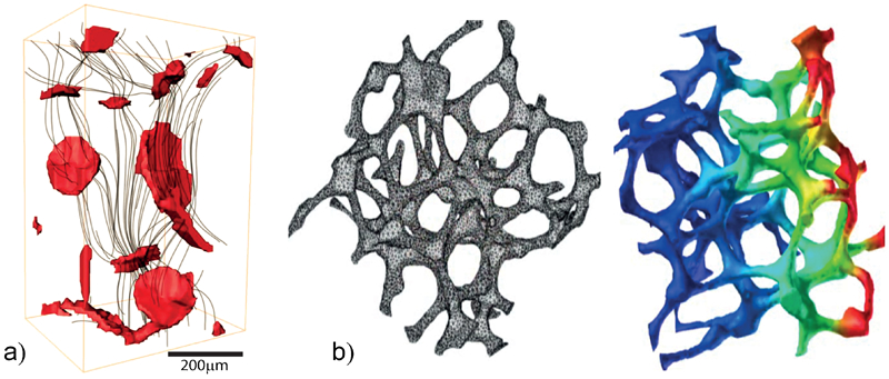
Tomograms can act as the basis for subsequent finite element predictions of performance. In a fluid dynamics is used to predict flow through the pores of a bioscaffold 409 and in b thermal transport through an open cell metallic foam (Alufoam) is computationally modelled (b courtesy P. M. Mummery)
Open cell metallic foams have great potential for removing heat. FE modelling can help to optimise the thermal transport v. weight v. mechanical properties v. geometry design challenge. Some studies have used actual reconstruction of microstructure as direct inputs for predicting thermal properties (mostly radiative and conductive properties). This has mainly been achieved for highly porous materials. 410–413 The thermal properties of nuclear graphite are also of technological concern and have been predicted directly from CT images. 414
Image based modelling of composites and multiphase materials
Another important category of materials particularly suited to the image based modelling are composites. Here the 3D structure of the reinforcement plays a first order role on the properties, and the direct meshing of tomograms can provide a feast of information on how the local and global properties relate to the microstructure. Work has been carried out on metal matrix composites 415–417 and fibre composites. 418–421 For example, Fig. 32 shows the typical results obtained using this method for a woven C–C composite. The figure illustrates how such a calculation yields both local and global information.
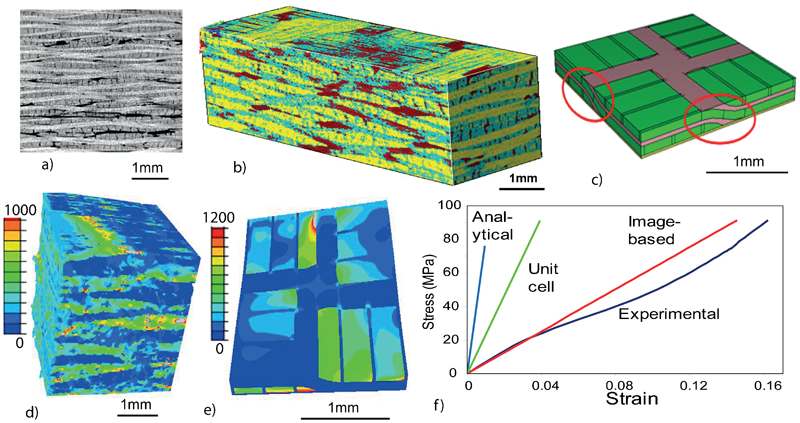
a Fully graphitised woven C–C composite. b an image based mesh showing red = porosity, blue = fibres+matrix in direction 1, yellow = fibres+matrix in direction 2 (courtesy Mummery), c the unit cell model extends (∼0·5×2×2 mm) Von Mises stress maps (in MPa) for d the image based mesh (∼2·5×2·5×2·5 mm) and the e unit cell and f the corresponding comparison of the elastic loading response for the actual composite and the various models 419
Finally, many bulk multiphase materials have also been analysed by CT image based modelling. Asphalt has been treated in several studies, 422–424 mortar by FFT in Ref. 368, multiphase ceramics in Refs. 365 and 425 and metals in Refs 370 and 426–430. In a recent study, Moulin et al. 431 suggest a physically based criterion for the fracture of complex shape inclusions embedded in a plastically deforming matrix. To apply this criterion, it is necessary to relate the stress concentration in the inclusions with the size of the volume over which this stress is reached.
In Berre et al., 432 the local value of the grey levels in the reconstructed tomograms are used to measure the local density in a nuclear graphite and to generate a multiphase model. The density is then used to modulate the Young's modulus and resistance of the local element and a finite element calculation is performed to account for these fluctuations and calculate the macroscopic behaviour for samples with different structures.
Polycrystal properties
Currently there is a great deal of interest in developing numerical models of materials behaviour at the grain scale. In the past, representative microstructures have been generated numerically 364 or by successive EBSD acquisition and destructive layer removal, 433–437 but this is time consuming, destructive and can only map a small volume.
Techniques capable of mapping grain orientations in 3D such as DCT (‘Crystal grain imaging’ section) are beginning to find application as a means of developing image based polycrystalline models to predict, for example, plastic deformation, microcracking and intergranular stress corrosion cracking. Further, in a number of cases it is possible to probe the micromechanical response of individual grains within a polycrystalline aggregate in situ.
Full 3D polycrystalline models can be input directly into crystal plasticity finite element models to predict the heterogeneity of plastic deformation at the intergranular level. 154,438 Others have focussed primarily on capturing the local reorientations arising from polycrystalline deformation, for example Wang et al. 439 have compared image based crystal plasticity predictions with in situ measurements of local reorientation made by 3D X-ray microscopy. The grain orientations can also affect the elastic development of thermal contraction stresses for materials having non-cubic crystals systems. Using DCT to build a polycrystalline model of alumina, Gonzalez et al. 332 have been able to predict the intergranular stresses arising from a combination of thermal residual stresses and mechanically applied compression. These predictions have been compared with strains inferred from the DCT measurements as well as the onset and location of intergranular microcracking recorded by conventional CT.
Grain scale models can also be used for analysing corrosion resistance already exposed in ‘Corrosion’ section. For intergranular stress corrosion, the grain boundary nature is important in terms of the susceptibility to corrosion. Simonovski et al. have taken DCT measurements of a polycrystalline stainless steel wire as the basis of an image based model (see ‘Polycrystal properties’ section) of intergranular stress corrosion cracking 440,441 and produced a mesh such as that shown in Fig. 33a . The experimentally determined lattice orientations were then employed to distinguish between resistant low-energy and susceptible high-energy grain boundaries in the model (Fig. 33b ).
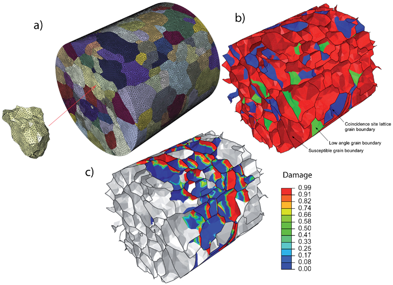
a FE mesh of the grain structure obtained by diffraction contrast tomography (DCT), b grain boundaries in the FE model: red: corrosion susceptible and green: low angle and blue: coincidence site lattice R3–R29 grain boundaries and c damage development in susceptible grain boundaries, red indicates fully developed crack 441
Concluding remarks and future trends
X-ray micro-CT has come a very long way over the last 20 years both in terms of spatial and temporal resolution, and the degree to which 3D images and 3D image sequences are quantified. It is now customary to spend 10–100× longer analysing datasets, compared to the time taken to capture them. Yet, many researchers are still only able to extract fairly rudimentary metrics to quantify the geometrical and temporal features of their images. The availability of open source and proprietary software toolboxes for image quantification are likely to expand the degree to which users can extract useful information about their samples non-destructively. Further, correlative tomography 81 analogous to correlative microscopy can bring together different measurements tools (e.g. X-ray tomography and fluorescence, scanning electron microscopy, etc) to image the same 3D features or tracking features over multiple length scales (e.g. the macroscopic and atomic nature of an inter-granular crack) will become more common. Whether a laboratory source or a synchrotron X-ray source will be used in the future will probably be determined less by spatial resolution than by the timescale of the events that one wishes to follow.
Currently limitations still remain; the great proportion of images are reconstructed using FBP. In cases that involve very noisy data or too few projections they would be better suited to emerging iterative reconstruction techniques. In many situations prior knowledge of the object (e.g. the number of phases, morphologies, etc.) should be incorporated into the reconstruction algorithm as prior information. Indeed in some circumstances, it may be possible to introduce certain morphological and phase fraction metrics into the interactive reconstruction so as to quantify the desired metrics directly as a part of the reconstruction process, e.g. to identify the optimal size of the pores in the volume image that are most consistent with the projection data, rather than leaving the quantification to a post-reconstruction image analysis step. Similarly, at present images come without error bars; iterative methods would allow us to evaluate the probability that water would permeate a foam or a composite would conduct electrically.
The widespread use of iterative reconstructions is unlikely until instrument providers either provide other reconstruction codes, or at least the necessary forward models, such that they can be seamlessly deployable on data collected on their instruments. Except for the simplest features (e.g. particle size, volume fraction, etc.), metrics obtained by image quantification such as permeability rarely come with error bars. Spatial resolutions of instruments are still on the whole poorly defined even for radiographs, let alone tomographs, and higher spatial resolutions are usually obtained at the sacrifice of small sample sizes. Region of interest tomography is still an emerging and underused strategy. 189
Nevertheless, looking back, there can be little doubt that the use and application of X-ray tomography is likely to grow significantly, especially for following structural evolution over time, whether during manufacturing, throughout service or in understanding the events leading to failure. In this respect, it promises to accelerate the materials design process and lead to safer, longer product lives.
Footnotes
Acknowledgements
The authors are particularly grateful to the instrument scientists and manufacturers who helped with compiling and discussing the form of Figs. 1 and 5 and comments from Profs. A. Mortensen, W. Lionheart and S. Stock as well as the referees. In addition PJW is grateful for funding from the BP International Centre for Advanced Materials, UoM and the EPSRC for funding the Manchester X-ray Imaging Facility under grants EP/F007906, EP/F028431 and EP/I02249X and for accommodation within the Research Complex at Harwell. New algorithms for the analysis of CT images are being developed as part of the Collaborative Computational Project CCPi being funded by EPSRC under the grant EP/J010456/1.