
Abstract
National Aeronautics and Space Administration Advanced Rapid Imaging Analysis (ARIA) Damage Proxy Maps (DPMs) are developed by the NASA Jet Propulsion Laboratory (NASA JPL) to identify potentially damaged areas based on interferometric coherence loss in Synthetic Aperture Radar (SAR) data. DPMs are typically based on data from Sentinel-1 satellites that orbit every 12 days, meaning that results can be provided within 1-2 weeks of an event. Although DPMs have been qualitatively validated as being able to detect surface effects of earthquakes, quantitative validations of their ability to differentiate damaged from undamaged areas and different types and levels of surface effects are lacking. We propose a framework for quantitative validation and apply it to surface fault rupture data from the 2019 Ridgecrest Earthquake sequence. The quantitative analyses take two forms: (1) the statistical distribution of a DPM index (
Keywords
Introduction
This study examines relationships between National Aeronautics and Space Administration Advanced Rapid Imaging Analysis (ARIA) Damage Proxy Maps (DPMs) and different levels of surface displacement following a major earthquake event. Since being developed in the early 2000s, DPMs have been utilized to rapidly detect “changes” on the surface of the earth following natural and anthropogenic disasters (Yun et al., 2015). Our aim is to quantitatively link, for the first time, the numerical index that is the basis for the maps to actual ground displacements.
DPMs are formulated with Synthetic Aperture Radar (SAR) data. Interferometric analyses of SAR data (InSAR) can be used to develop interferograms, which measure radar wave phase change as a function of position on the earth. With information on wave frequency and propagation velocity, phase change between two times at a given location can be converted to displacements on the earth’s surface at that location, down to a minimum resolvable displacement of 1/32 of a SAR wavelength. In the case of the Copernicus Sentinel-1 satellites, which utilize C-band SAR waves, the implied minimum detectable displacement is about 0.175 cm based on a 5.6 cm wavelength (Burgmann et al., 2000; Massonnet and Feigl, 1998).
Prior work suggests a potential theoretical upper limit to the displacement levels that can be distinguished using InSAR data. When surface displacements in the line of sight (LoS) direction (i.e. from a satellite to the ground surface) exceed half of a SAR wavelength (for Sentinel-1 which utilizes C-band SAR waves, about 2.8 cm) over the length of a SAR pixel, coherence loss occurs and displacement changes can no longer be resolved (Peltzer et al., 1994). Coherence loss is a term used in InSAR literature that refers to displacement change not being resolvable. In addition to excessive phase shift due to large displacements, coherence loss can also result from re-orientation of scatterers within a specified area on the earth’s surface (i.e. pixel) between the acquisition times of the two SAR images. DPMs aggregate coherence loss across a specified area (collection or analysis window of adjacent pixels), which is converted using different algorithms to an index that ranges from -1.0 to 1.0 for DPM1 and 0.0 to 1.0 for DPM2, with higher values corresponding to more coherence loss in both instances. The DPM is a map of this index, converted to color, that provides a visual representation of “change” from before an event occurred to after it. It is reasonable to assume that DPMs would be able to identify areas where surface fault rupture exceeds half a SAR wavelength. However, it is harder (if not impossible) to measure scatterer reorientation. Due to these multiple potential causes of coherence loss, only one of which is related to ground displacement, formal validation is needed to see if displacement can be resolved from DPM indices.
DPMs have been qualitatively evaluated for their ability to detect landslides (Yun et al., 2015), building damage (Sextos et al., 2018; Yun et al., 2015), and surface fault rupture (Fielding et al., 2005). Prior to the present work, validations of DPMs were mostly performed using Boolean (and/or multi-class) labels for the ground truth data and the presence of colored DPM pixels (whose DPM index values are not explicitly stated) to test the ability of DPMs to identify damage. The only prior quantitative validation using actual measurements and DPM index values focused on their ability to detect structural damage and blast effects on building facades (Sadek et al., 2022). In this paper, we seek to quantitatively validate DPMs’ ability to detect different levels of surface displacement. We introduce a process to establish links between DPM index and (1) the binary distinction of whether displacement was or was not recorded at a given location and (2) the amount of displacement. We anticipate that such numerical procedures may be of general interest, even for other remote sensing technologies (Dell’Acqua and Gamba, 2012). We utilize a dataset gathered following the 2019 Ridgecrest Earthquake sequence consisting of surface fault rupture measurements along the major fault ruptures associated with both the
Following this introduction, we describe the bases for different types of DPMs, present the data that is considered along with the analysis methods, and conclude with a presentation and discussion of the results.
Damage proxy maps
NASA-JPL produces two types of DPMs (DPM1 and DPM2). As noted in the Introduction, for each a DPM index is computed from SAR data for a given pixel. The procedures used for these calculations are described below. These descriptions have been adapted from relevant literature, with certain details that are important for conceptual understanding more clearly stated and some mathematical details corrected (specifically, Eq. 4).
DPM1
The DPM1 index is based on the difference in interferometric coherence of two pairs of SAR images, one pre-event pair (i.e. a pair of SAR images acquired before the disruptive event) and one co-event pair (i.e. a pair of SAR images comprising a pre-event image and an image taken after the disruptive event). Interferometric coherence is a measure of the consistency in radar wave phase between two SAR images of the same area at different times. Interferometric coherence is measured for each pixel using the magnitude of complex coherence (Fielding et al., 2005; Rosen et al., 2000),
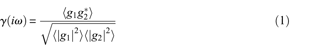
where g 1 and g 2 describe the complex-valued and frequency-dependent radar wave properties recorded during different passes of a satellite over a given location, each of which can be described by,

where index
The spatial integration represented by the 〈〉 operator computes power spectral densities (and coherence) across a window defined by a particular number of SAR pixels. For Sentinel-1, SAR pixels have dimensions of roughly 3 × 14 m and a typical window size is 16 × 4. As a result, integration occurs across a window roughly 48 m × 56 m in size. Some authors use the term “spatial correlation” for the interferometric coherence because the spatial integration is a measure of the spatial correlation of the phase values (Fielding et al., 2005).
The DPM1 index (

where
To understand the physical meaning of
The DPM1 index can be ineffective for cases with low pre-event coherence because
DPM2
DPM2 uses the amplitude of complex coherence as given by Eq. (1). However, while DPM1 uses two pairs of SAR images (i.e. a pre-event pair and a co-event pair), DPM2s uses many pairs of SAR images (i.e. multiple pre-event pairs and at least one co-event pair). By using many pre-event images to characterize coherence, a more robust baseline is established for temporal coherence loss difference calculations. Zebker and Villasenor (1992) and Jung et al. (2016) describe a number of factors that influence coherence, including non-temporal factors and temporal factors.
Temporal decorrelation is defined as the decorrelation caused by abrupt (sudden) events, which may have small or large impacts (e.g. person walking by or earthquake, respectively) or by gradual changes such as the growth of vegetation (Jung et al., 2018; Zebker and Villasenor, 1992). Temporal decorrelation is a measure of abrupt or gradual changes of the positions of scatterers and/or radar targets on the ground. Temporal decorrelation is influenced by three contributing factors:
Temporally-correlated coherence (
Temporally-uncorrelated coherence (similarly
Other decorrelation factors (e.g. geometric, thermal, volumetric; Fielding et al., 2005).
Sources in factor #3 are negligible in interferometric SAR applications such as those we are describing in this paper (i.e. Jung et al., 2018). As such, temporal decorrelation can be solely described by the temporally-correlated and temporally-uncorrelated terms.
The temporally-correlated coherence has been observed to decay exponentially as the time window used for the pre-event analyses lengthens, which can be referred to as an interval length effect (Jung et al., 2018). This coherence loss is generally thought to result from a gradual accumulation of changes in vegetation or other surface materials. To account for this length effect, DPM2 uses an exponential temporal decorrelation model (i.e. Eq. (15) in Jung et al., 2018). This model is used to de-trend the exponential decaying term of temporal decorrelation. The remaining portion of the temporal decorrelation, after removing the model for the interval length effect, is
The DPM2 index,
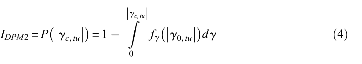
To conceptualize the meaning of Eq. (4), consider the case of
Although DPM2 is considered to provide a methodological improvement to DPM1, the differences might be anticipated to be modest for the Ridgecrest case because of its flat, desert environment. The DPM2 method involves a much larger amount of data processing than the DPM1 method.
Ground movement data and DPMs
Field reconnaissance data
The surface disruption event considered in this paper is from an earthquake sequence near Ridgecrest, California on July 4 and 5, 2019. The sequence began on July 4 with a
Following the earthquake sequence, teams led by the USGS gathered 522 surface fault rupture measurements along the approximately 18 km and 52 km of fault rupture from the
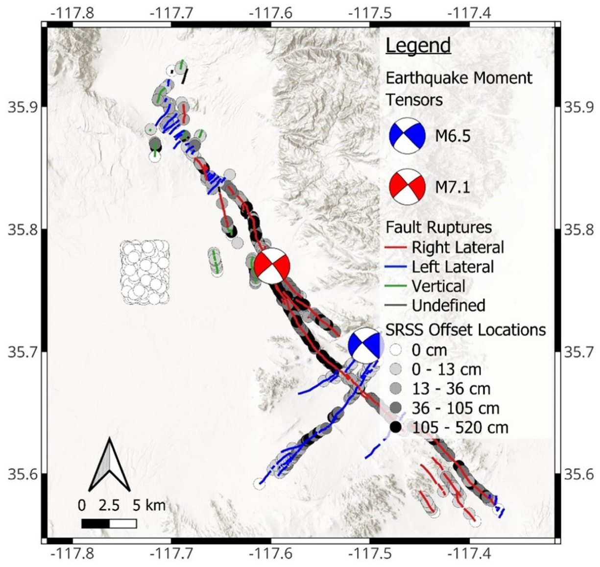
Fault measurement locations and “true zero displacement” points from 2019 Ridgecrest earthquake sequence. The moment tensors were generated using the Python library, ObsPy (Beyreuther et al., 2010), using moment tensor data from the USGS event page.
The dataset from DuRoss et al. (2020b) is essentially complete for locations of ground cracks. However, it is not complete for displacement vectors (e.g. there are areas where surface fault rupture features were observed, without associated vector measurements). It also contains few zero displacement data points (26 points). To achieve balance in the dataset between data points with and without measured displacements, 260 “true zero displacement” points were added to the dataset based on observations from on-ground inspections and helicopter overflights. The selected true zero data points are all located close to each other in a relatively small area. Before selecting these data points, we pre-selected a larger number of candidate areas. However, areas other than the selected one presented ground failure features (e.g. landslides, liquefaction, ground cracks, and/or surface fault rupture features) or were outside reconnaissance boundaries. The selected true zero area is the only one for which we are sure that no ground failure occurred at these locations (i.e. at these locations post-earthquake observations confirmed that ground failure did not occur; Figure 1 of Zimmaro et al., 2020). The number of “true zero” points added was selected to balance displacements (i.e. horizontal, vertical, and crack width) by percentiles into five equally size bins (i.e. null, >0-25th percentile, 25-50th percentile, 50-75th percentile, and 75-100th percentile).
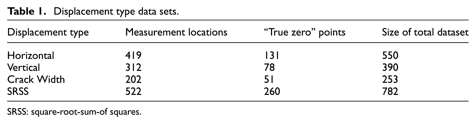
The displacement data can be represented in different ways for the comparisons to DPM indices. We consider the along-strike horizontal-component, vertical-component, crack width, and the square-root-sum-of squares (SRSS) of the horizontal-components, vertical-components, and crack width offsets. When a displacement measurements type was missing at a given location (typically in the vertical or crack width fields), they were taken as zero. Table 1 summarizes the numbers of displacement data points that were considered in the analyses presented subsequently.
Displacement type data sets.
SRSS: square-root-sum-of squares.
DPMs
After the earthquake sequence, on 11 July 2019, a DPM1 was released that mapped the heavily affected portion of California from these events, including Searles Lake. The DPM1 index calculation used a 16 × 4 window (DPM1-16 × 4) of SAR pixels and was geocoded and resampled to have the same resolution as the SRTM DEM (1-arcsecond or approximately 30 m pixel spacing). The map was created using ascending track SAR data from the Copernicus Sentinel-1 satellites, operated by the European Space Agency (See Table A2). Interferometric processing was performed with the ISCE2 package (Rosen et al., 2012). A first version of the map was made publicly available through the ARIA event page (https://aria-share.jpl.nasa.gov/20190704-0705-Searles_Valley_CA_EQs/DPM/). The DPM1 initially available on the ARIA event page was formatted in a manner that favors readability for event responders. That map was prepared by making DPM indexes transparent below a pre-defined threshold and color-coded when index values were above this threshold. In our analyses we used “raw” DPM maps. In these maps, each pixel in the calculation domain is assigned a DPM index (i.e. they are all visible and none of them is transparent). For this study, four raw DPMs were generated by NASA-JPL: a raw DPM1 version of that initially published on the ARIA event page (DPM1-16 × 4), a DPM1 utilizing the same ascending track Sentinel-1 data and a smaller calculation window of 8 × 2 (DPM1-8 × 2), and two DPM2s derived from ascending and descending satellite tracks (denoted DPM2-TA and DPM2-TD, respectively) that both used the regular 16 × 4 pixel windows (See Table A2). As a result, including DPM1-16 × 4, four DPMs were considered in this study (available at the JPL Open Repository; https://doi.org/10.48577/jpl.0LBWZG). This facilitated comparison between DPM1 and DPM2, between different DPM1 window sizes, and between DPM2s from ascending and descending tracks.
The reason different flight track directions are considered for DPM2s is that it can affect DPM accuracy in areas with topographic features. In the present case, where the fault ruptured in flat areas, we do not expect to see significant differences between the alternate DPM2s.
Data analysis and results
Using the Geographic Information System (GIS) tool QGIS, 60 m diameter buffers were generated surrounding all 782 locations with either surface fault displacements or zero displacements (Figure 1). This buffer diameter was chosen because it is roughly equivalent to the width of the default, 16 × 4 SAR pixel spatial integration window (56 m). For each DPM type, the mean DPM index within the 60 m buffer around each measurement point was computed for the analyses presented in this section. This choice was made because we consider the mean index to be representative of the index values within each buffer.
For each displacement type, the different DPMs were evaluated with respect to the following criteria:
The analyses performed to evaluate DPMs’ ability to distinguish these displacement amounts were evaluated using box and whisker and fragility analyses, as described next.
Box and Whisker analyses
The first comparisons between DPM indices and the measured surface rupture displacements are presented through box and whisker plots (i.e. graphs showing groups of numerical data where a box represents the 25th and 75th percentiles, whiskers represent the 95th and 5th percentiles, and a line inside the box represents the median value of that bin). Through these figures, performance metrics were quantified which give a means of directly quantifying the performance of the various DPMs at detecting different offset levels.
Box and whisker analyses were conducted on every displacement type and DPM and repeated to address each of the three criteria listed above. The available data were separated into bins depending on the criterion being investigated, as follows:
For Criterion 1, two bins were considered, one consisting of buffers where the displacement was greater than 0 cm and the other where the offset was either measured or inferred to be zero.
For Criterion 2, only locations with non-zero displacements were considered and two bins with different displacement percentile ranges were used (> 0-50th, 50-100th).
For Criterion 3, again only non-zero displacement locations were considered, and four displacement percentile bins were used (> 0-25th, 25-50th, 50-75th, and 75-100th).
The displacements corresponding to different percentiles are given in Table 2 for each displacement type.
Displacement percentiles.
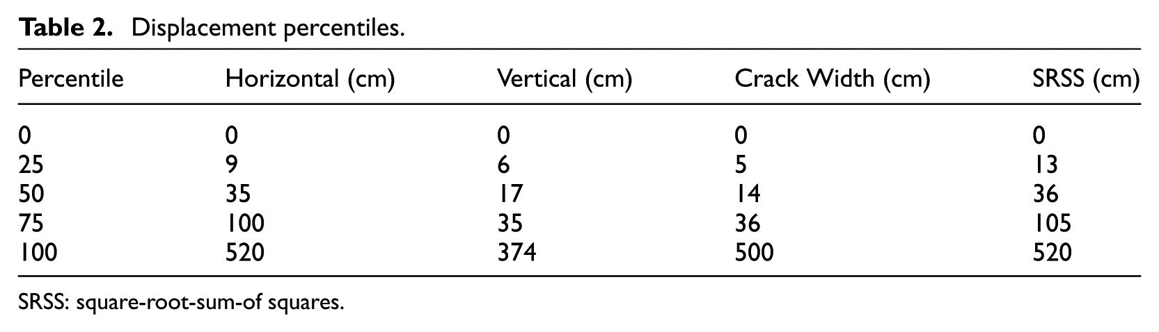
SRSS: square-root-sum-of squares.
Figure 2 shows a histogram of the 522 measured displacements (using SRSS), including a bin showing the number of observations for zero displacements and the bounds of the percentile-based bins.
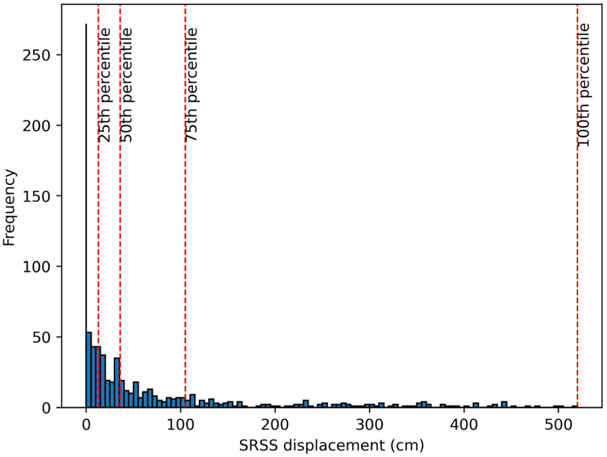
Histogram for SRSS fault measurement locations and “true zero displacement” points from 2019 Ridgecrest earthquake sequence.
Figures 3 and 4 present box and whisker plots for SRSS displacements evaluated using Criteria 1 and 2; four plots are shown in each case for the four considered DPM types. Outliers are represented with black circles on the ends of each whisker. Figure 3 shows that there is a significant gap between the
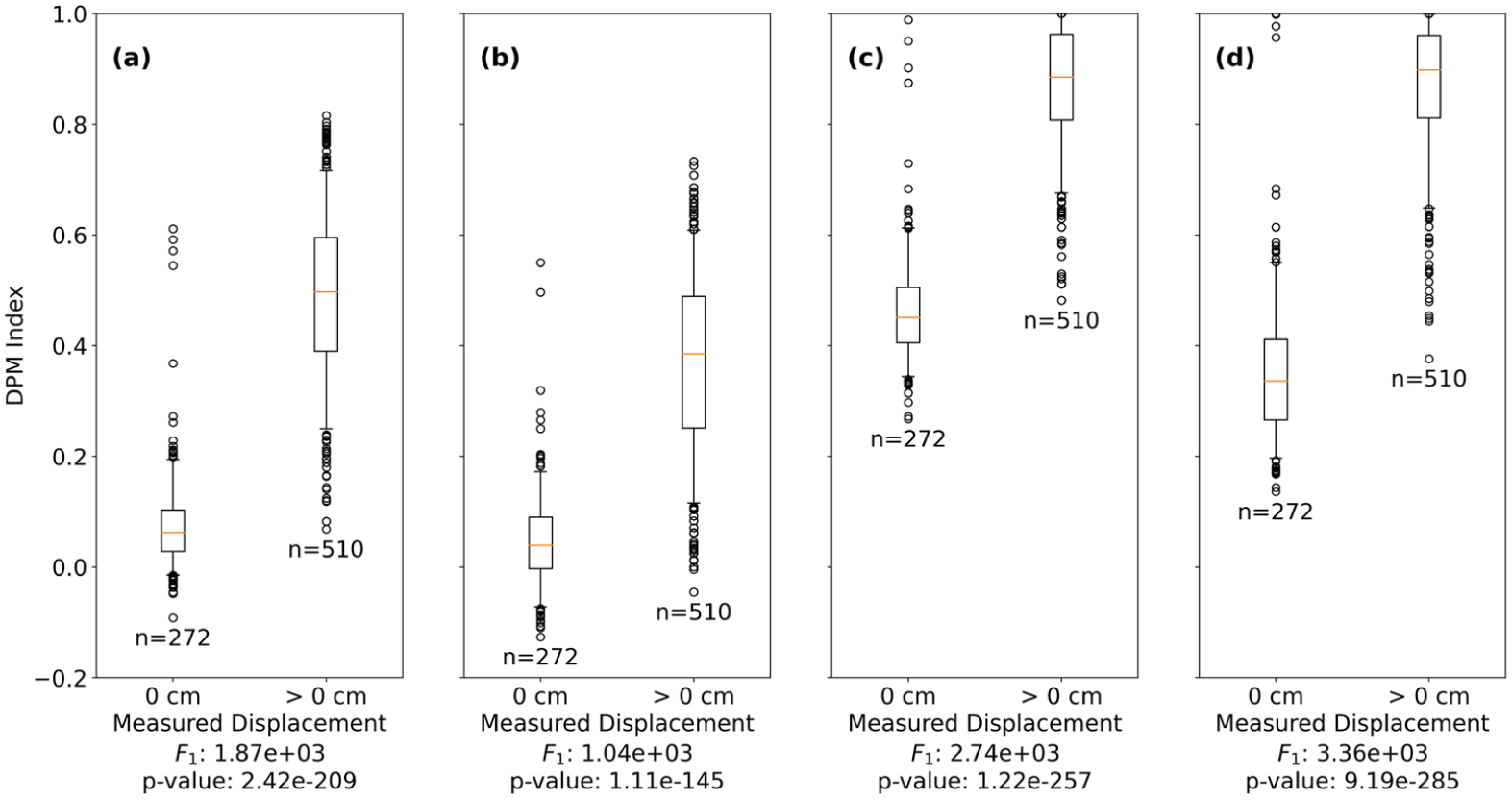
Box and whisker plots for SRSS displacements comparing “no displacement” vs “some displacement”: (a) DPM1-16 × 4, (b) DPM1-8 × 2, (c) DPM2-TA, and (d) DPM2-TD.
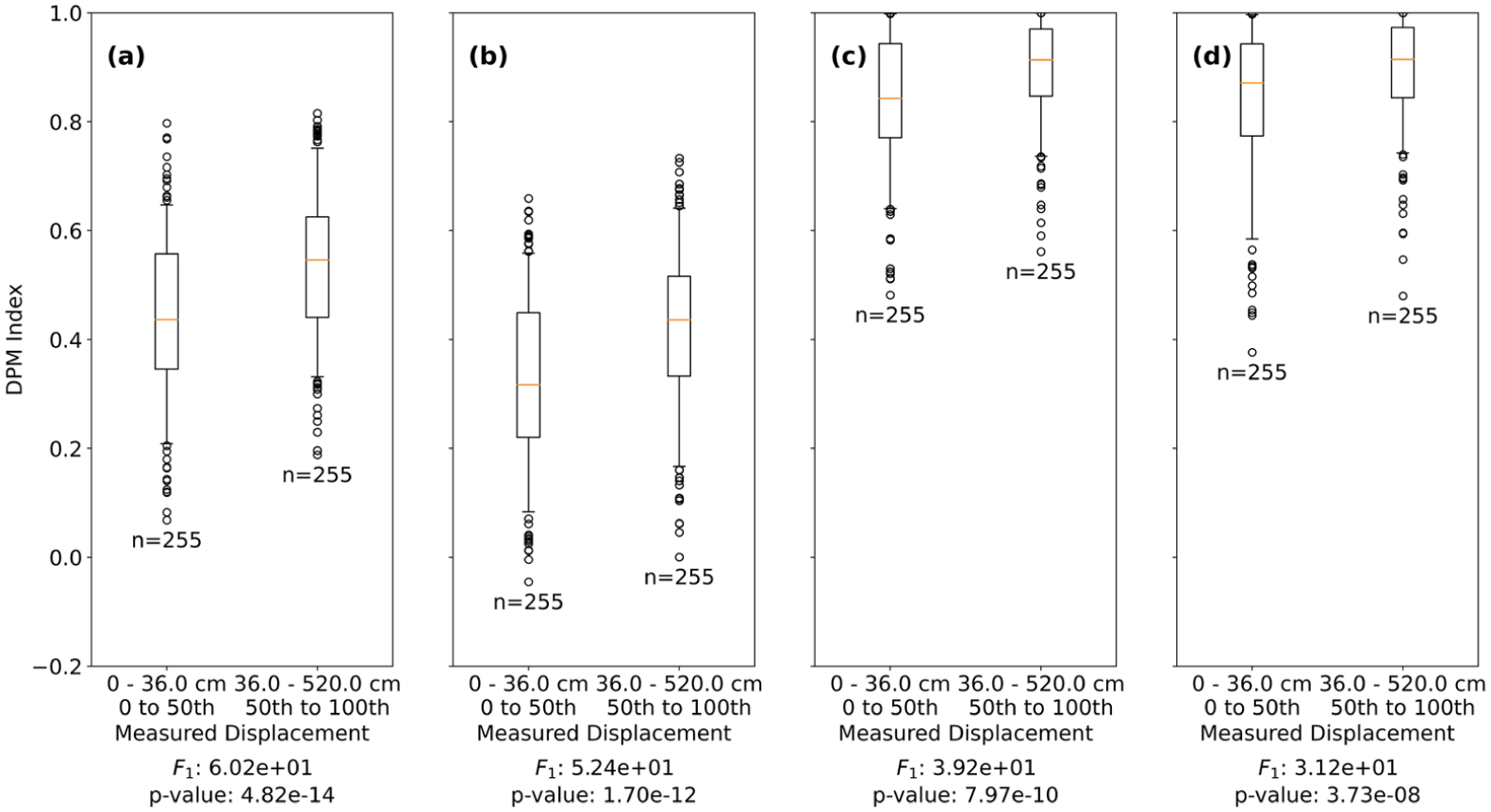
Box and whisker plots for SRSS displacements comparing “moderate displacement” vs “large displacement”: (a) DPM1-16 × 4, (b) DPM1-8 × 2, (c) DPM2-TA, and (d) DPM2-TD.
To evaluate the distinctions between data distributions in a quantitative manner, we use an F-test (Snedecor and Cochran, 1989). This test compares the statistical performance of sub-models (e.g. the two distributions for a given DPM type in either of Figures 3 or 4) with that of a full model (i.e. the combination of the two distributions). The F-test assumes that the bins of data are normally distributed and have similar variances, both of which are satisfied for all of the data bins generated for this analysis. For a given distribution, the median
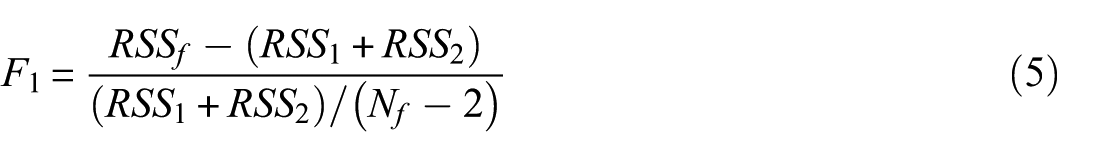
where N
f
is the number of buffers in the dataset. This F-statistic can be compared to the F distribution to evaluate a significance level (p) for the test. This was done utilizing the “f-one way” function from the Python library SciPy. Small values of F
1
and large values of p (> 0.05) suggest that the models are not distinct. In Figures 3 and 4, the
Figure 5 presents box and whisker plots for the SRSS displacements evaluated using Criterion 3 (i.e. to check DPMs performances for various displacement bins). Median
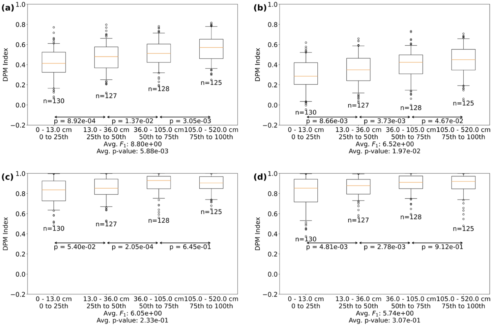
Box and whisker plots for SRSS displacements for different displacement levels: (a) DPM1-16 × 4, (b) DPM1-8 × 2, (c) DPM2-TA, and (d) DPM2-TD.
Although not shown here for brevity, similar results are obtained for horizontal displacements. The DPM indices were generally less effective at distinguishing vertical displacements and offsets. This is likely a consequence of fault rupture having been strike-slip with predominantly horizontal displacement. Box and whisker plots for each displacement metric and corresponding F-test results are provided in O’Donnell et al. (2024).
Overall, the results suggest that both DPM2s are marginally better than both DPM1s at distinguishing between areas with no surface fault rupture and some surface fault rupture, although each DPM type is effective from a statistical perspective. However, both DPM1s are marginally better than the DPM2s at distinguishing between moderate- and large surface fault rupture displacements. These results suggest that in a flat, desert environment with little vegetation, DPM1s and DPM2s are both effective but may be best used in tandem.
Fragility analysis
Additional comparisons between DPM indices and measured surface rupture displacements are presented using fragility functions, which are curves relating the probability of a certain damage threshold being exceeded to a demand parameter or a proxy (Baker, 2015; Porter et al., 2007).
For each DPM and displacement type, fragility functions were derived conditioned on
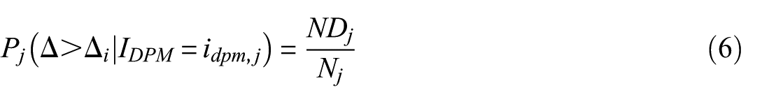
where
The blue bars in Figure 6 show the variation of
Bar chart showing probabilities of exceeding null displacement for buffers with variable levels of
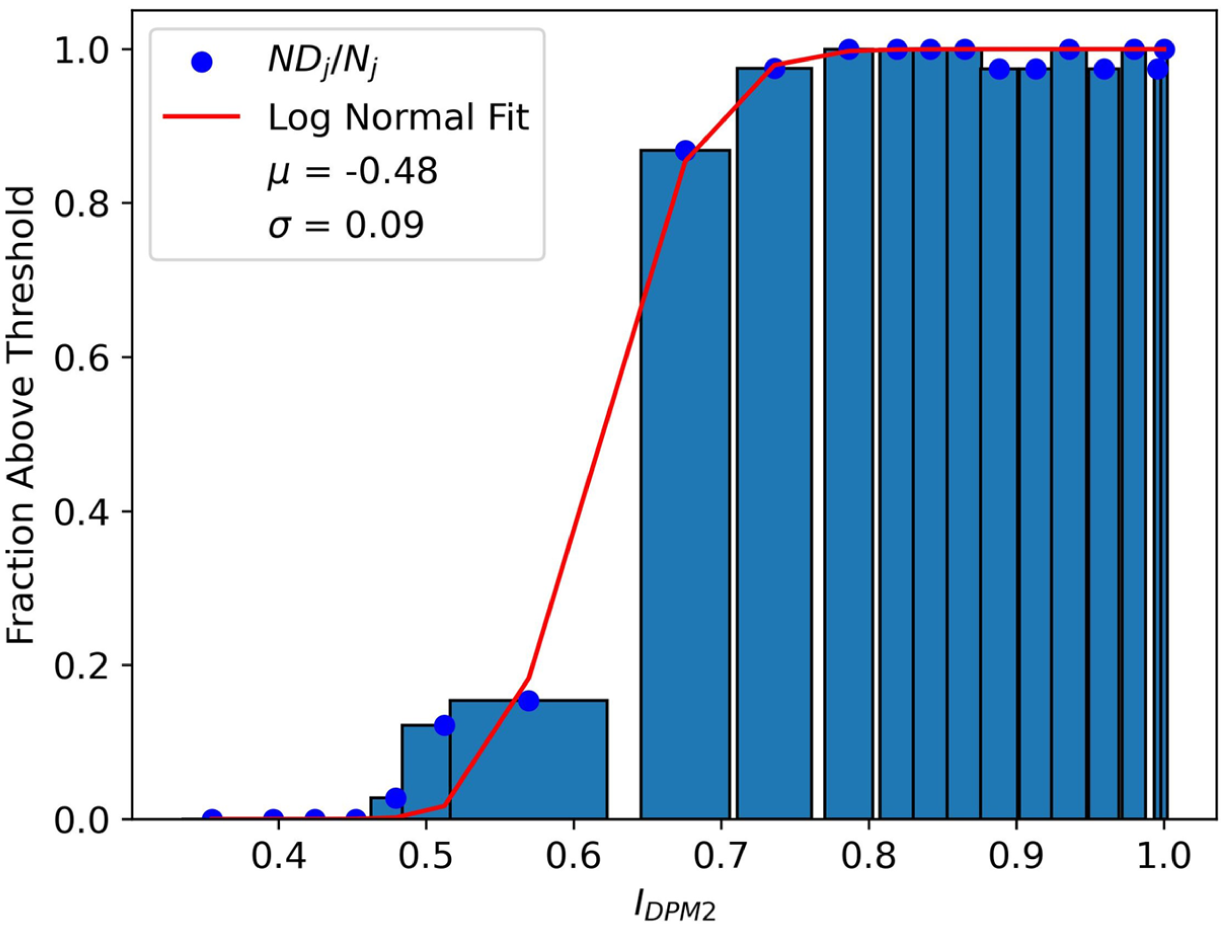
Figure 7 shows a similarly derived fragility function for a threshold displacement of
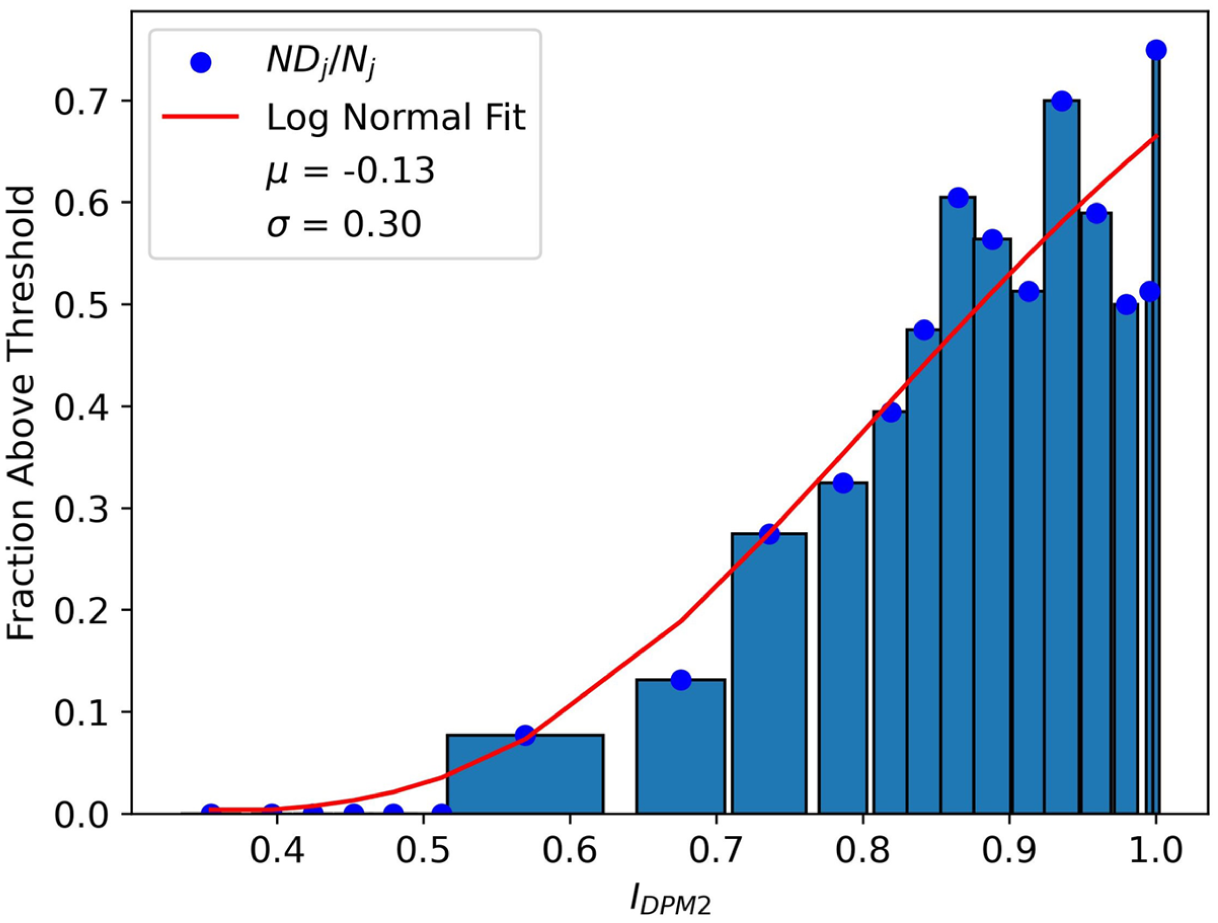
Bar chart showing probabilities of exceeding 36 cm displacement for buffers with variable levels of
Fragility analyses were repeated for each displacement type and DPM type and for various displacement levels corresponding to different percentiles from Table 2. Table A1 (in the electronic supplement to this paper) reports means and standard deviations of log-normal CDF fragility functions for each analyzed displacement metric and DPM type. As shown in Figure 8, DPM indices demonstrate stronger predictive power (lower
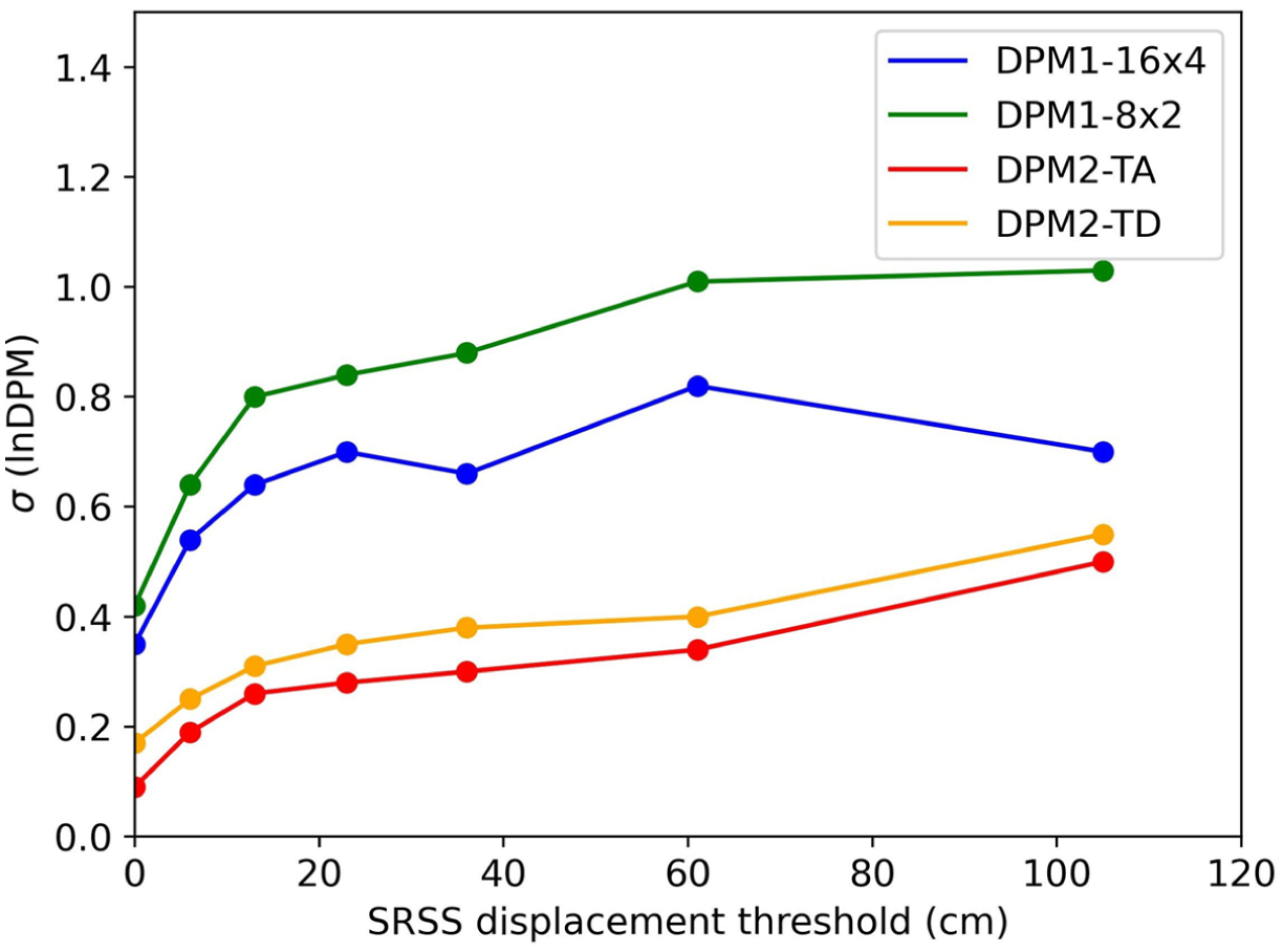
Dependence of
Optimal threshold analysis
An important outcome of the fragility analyses presented in the previous section is the level of DPM index that effectively differentiates buffers at which a displacement threshold is and is not exceeded. An intuitive choice for this threshold is the index value (
We take the optimal threshold as the DPM index that differentiates buffers with displacements below and above the displacement threshold. To illustrate the process for optimal threshold identification, consider for example a displacement threshold of zero and
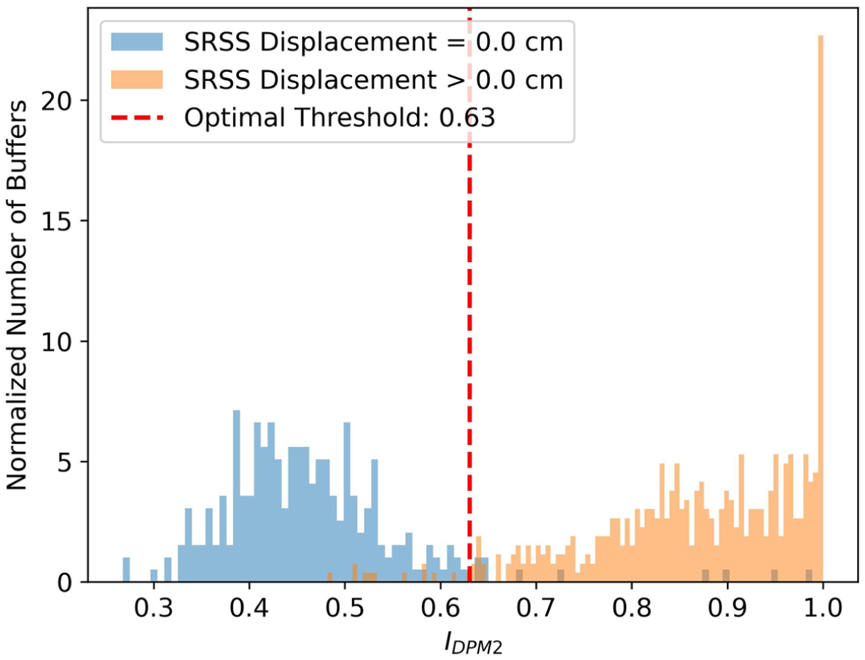
Histograms of DPM indices for buffers with displacements below and above a displacement threshold value that are used to identify an optimal DPM index threshold. Data shown are for a zero-displacement threshold and
The value of
Application of fragility curves for predictions of fault rupture displacement probabilities
The fragility curves in Figures 6 and 7 can be used to predict the probability of exceeding null or 36 cm displacement levels conditional on
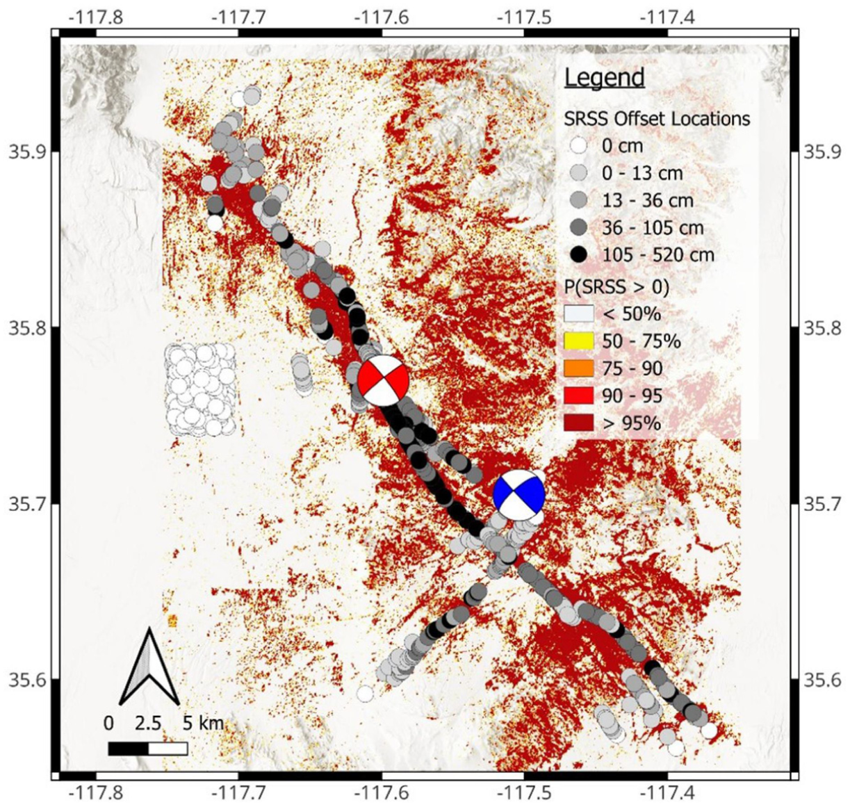
Map showing locations and amounts of SRSS displacements overlain on pixels colored to indicate probabilities of exceeding null displacement conditioned on
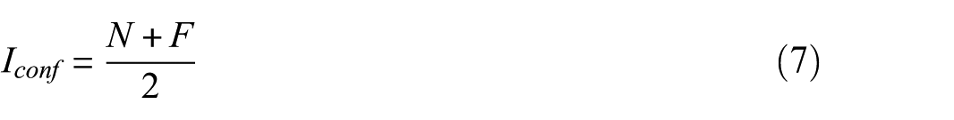
Model performance is commonly evaluated using the performance metrics “Recall” and “Precision” that are defined as follows:
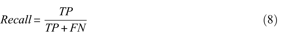
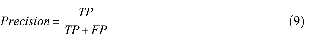
where TP = true positive, FN = false negative, and FP = false positive. The meaning of recall is the fraction of positive incidents (in this case, measured displacements that exceed the threshold) that are correctly predicted by the
The threshold probability used with the fragility model is subjective. In the case of the
Using the 27% probability level with the
Figure 11a shows the performance of the
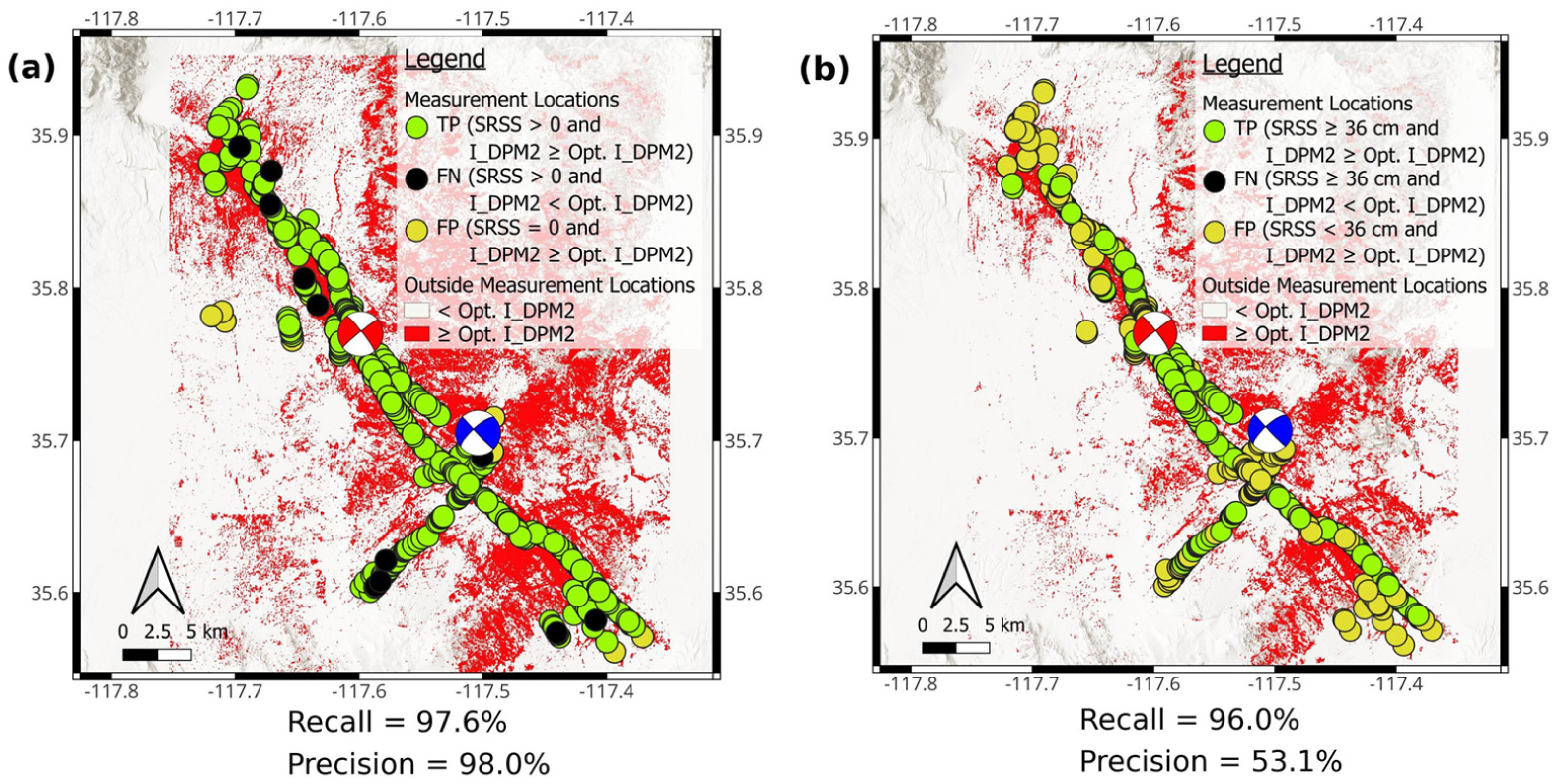
Map of
To more clearly show the spatial relationships between observed displacements and predicted exceedance probabilities, Figure 12 shows these quantities as a function of along-strike position for the (b) the Paxton Ranch fault (
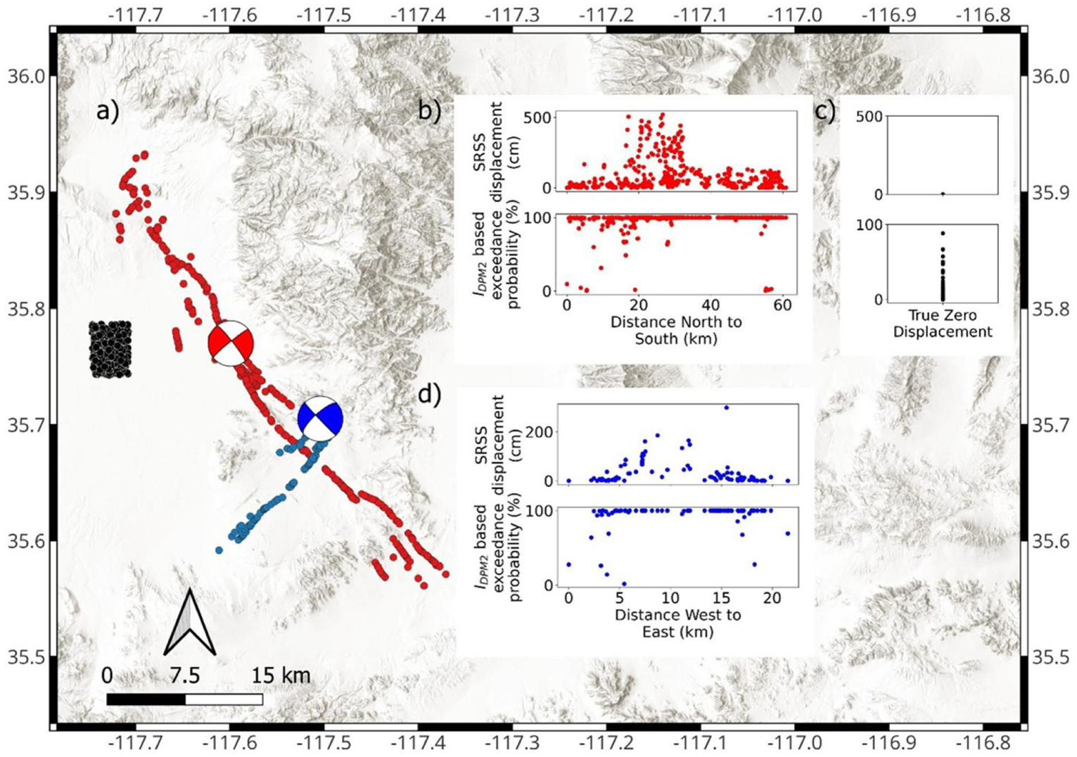
(a) SRSS fault measurement locations with epicenters for Paxton Ranch fault
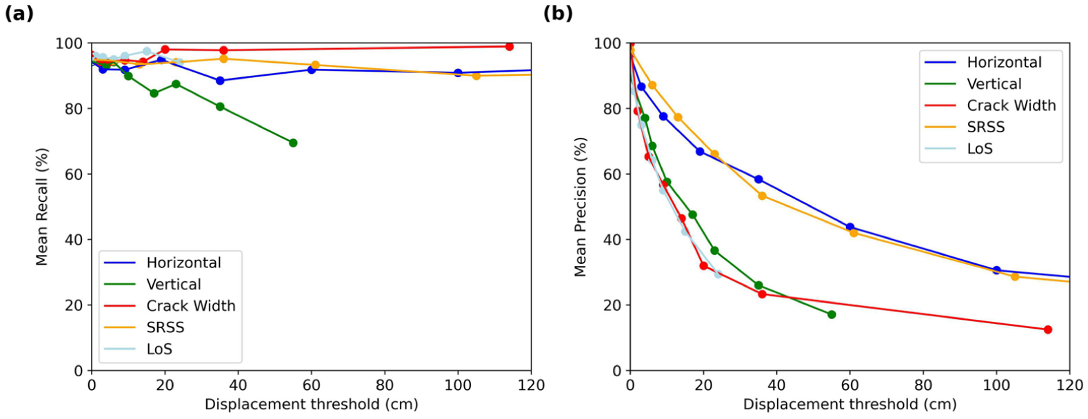
In Figure 13, we extend the performance metrics discussed above for different DPM types and a range of

Performance metrics vs displacement threshold,
The performance metrics considered to this point have been based on fragility curves derived for the SRSS displacement type. To investigate sensitivity to displacement type, we average metrics across all DPMs (due to the similarity of performance metrics across DPMs; Figure 13), and plot in Figure 14 the resulting average performance metric against displacement threshold. The performance metrics derived for displacements in the line of sight (LoS) direction associated with the ascending Sentinel-1 track are of special interest because SAR wave phase change, and hence
Average performance metrics vs displacement threshold,
Conclusion
We quantify the performance of four types of SAR-based Damage Proxy Maps (DPMs) using surface fault rupture displacement data collected following the 2019 Ridgecrest earthquake sequence. DPM results for a given location (pixel) are represented using DPM indices (
Four DPM types were considered: two DPM1 types based on different window sizes (representing different resolution levels) and two DPM2s based on different satellite orbital motions (i.e. ascending and descending). Box and whisker plots indicating
We examined relationships between IDPM values and probabilities of exceeding various threshold displacements, which were developed empirically and then fit using log-normal cumulative distributions functions. The standard deviation terms in those functions indicate the predictive power of the
Although our analyses are based on an individual earthquake sequence, we are able to provide quantitative insights into the applicability and use of DPMs. This research demonstrates both the value and the limitations of DPM indices for identifying areas of ground deformation. While DPM2 has some clear advantages, the narrow range of its index (
Data and resources
The surface fault rupture data used in this paper is available at DuRoss et al. (2020b). Moment tensor data for the 2019 Ridgecrest earthquake sequence are from the USGS event page, available at: https://earthquake.usgs.gov/earthquakes/eventpage/ci38457511/executive (last accessed on 10 March 2025). The DEM used in this study is from the 1-arc sec data from the USGS EROS Center (2018). Preliminary DPMs are available at the National Aeronautics and Space Administration (NASA) Advanced Rapid Imaging and Analysis (ARIA) Jet Propulsion Laboratory (JPL) event page at https://aria-share.jpl.nasa.gov/20190704-0705-Searles_Valley_CA_EQs/DPM/. The DPMs used in this analysis are available from the JPL Open Repository (DOI: 10.48577/jpl.0LBWZG).
Footnotes
Appendix
Synthetic aperture radar (SAR) scenes analyzed for DPM1 products.
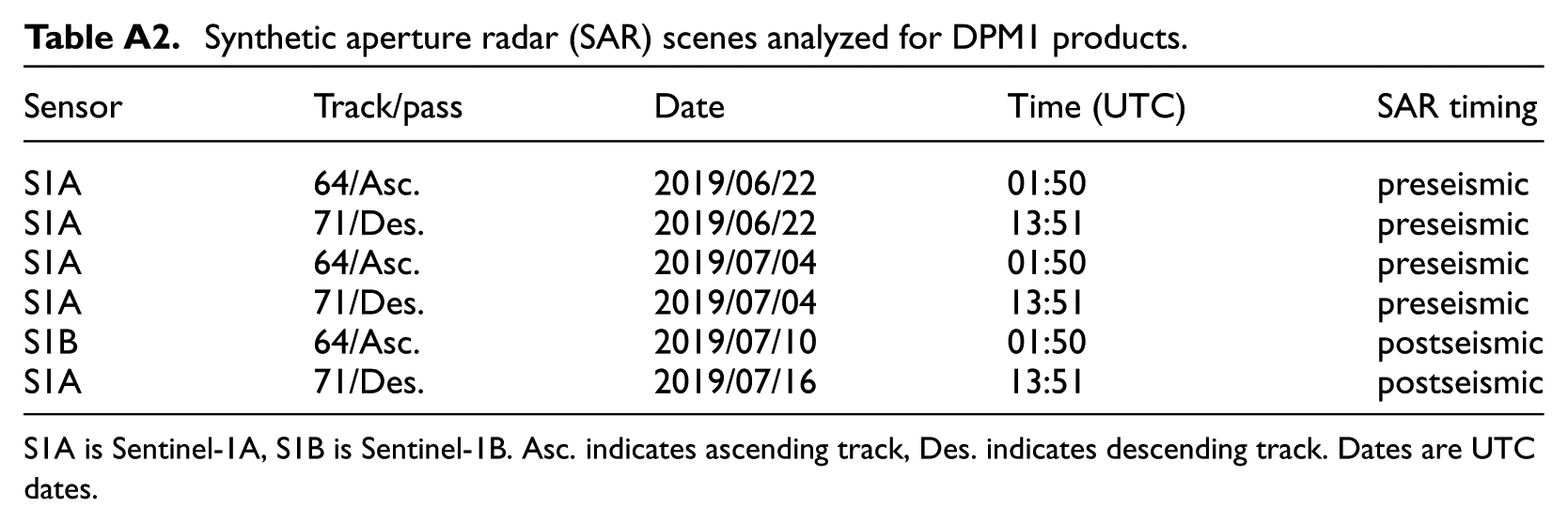
| Sensor | Track/pass | Date | Time (UTC) | SAR timing |
|---|---|---|---|---|
| S1A | 64/Asc. | 2019/06/22 | 01:50 | preseismic |
| S1A | 71/Des. | 2019/06/22 | 13:51 | preseismic |
| S1A | 64/Asc. | 2019/07/04 | 01:50 | preseismic |
| S1A | 71/Des. | 2019/07/04 | 13:51 | preseismic |
| S1B | 64/Asc. | 2019/07/10 | 01:50 | postseismic |
| S1A | 71/Des. | 2019/07/16 | 13:51 | postseismic |
S1A is Sentinel-1A, S1B is Sentinel-1B. Asc. indicates ascending track, Des. indicates descending track. Dates are UTC dates.
Acknowledgements
We acknowledge ESA for processing the Copernicus Sentinel-1 level-1 images available through the Alaska Satellite Facility (ASF) at no cost. This work contains modified Copernicus data from the Sentinel-1 satellites processed by the ESA. Part of the research was carried out at the Jet Propulsion Laboratory, California Institute of Technology, under a contract with the National Aeronautics and Space Administration (80NM0018D0004). We thank Dr. Sang-Ho Yun at the Remote Sensing Lab, Earth Observatory of Singapore and Nanyang Technological University (NTU) for processing DPM1 used in this study. We would also like to thank Dr. Jungkyo Jung of the Jet Propulsion Laboratory for his assistance in understanding the functional details of DPM2 and for processing DPM 2 used in this study. We appreciate the constructive feedback from Dr. Eleanor Ainscoe and one anonymous reviewer along with the Associate Editor, which have improved the manuscript.
Author note
The views and conclusions presented in this article are those of the authors and do not reflect the policy of the U.S. Government.
Declaration of conflicting interests
The author(s) declared no potential conflicts of interest with respect to the research, authorship, and/or publication of this article.
Funding
The author(s) disclosed receipt of the following financial support for the research, authorship, and/or publication of this article: Funding for this study was provided by the National Aeronautics and Space Administration (Subcontract no. 1650617). Partial support for the first author was also provided by the UCLA Civil & Environmental Engineering Department. This support is gratefully acknowledged.