
Abstract
Continuous advancements in scientific and engineering understanding of earthquake phenomena, combined with the associated development of representative physics-based models, is providing a foundation for high-performance, fault-to-structure earthquake simulations. However, regional-scale applications of high-performance models have been challenged by the computational requirements at the resolutions required for engineering risk assessments. The EarthQuake SIMulation (EQSIM) framework, a software application development under the US Department of Energy (DOE) Exascale Computing Project, is focused on overcoming the existing computational barriers and enabling routine regional-scale simulations at resolutions relevant to a breadth of engineered systems. This multidisciplinary software development—drawing upon expertise in geophysics, engineering, applied math and computer science—is preparing the advanced computational workflow necessary to fully exploit the DOE’s exaflop computer platforms coming online in the 2023 to 2024 timeframe. Achievement of the computational performance required for high-resolution regional models containing upward of hundreds of billions to trillions of model grid points requires numerical efficiency in every phase of a regional simulation. This includes run time start-up and regional model generation, effective distribution of the computational workload across thousands of computer nodes, efficient coupling of regional geophysics and local engineering models, and application-tailored highly efficient transfer, storage, and interrogation of very large volumes of simulation data. This article summarizes the most recent advancements and refinements incorporated in the workflow design for the EQSIM integrated fault-to-structure framework, which are based on extensive numerical testing across multiple graphics processing unit (GPU)-accelerated platforms, and demonstrates the computational performance achieved on the world’s first exaflop computer platform through representative regional-scale earthquake simulations for the San Francisco Bay Area in California, USA.
Keywords
Introduction
A number of challenges and uncertainties persist in the performance of earthquake hazard and risk assessments. Empirical ground motion models, widely employed in engineering practice for seismic hazard assessments, are based on sparse data sets and typically must utilize data from many locations other than the region of interest. Such models can provide key insight on the intensity of ground motions that might be anticipated in a statistical sense but cannot be expected to represent the complex site-to-site variability of ground motion waveforms resulting from fault rupture seismic wave radiation patterns, propagation path, and local site effects. To address the challenges associated with accurate prediction of site-specific motions across a selected region, interest continues to grow in the development of physics-based high-performance regional simulation models. In addition, to create tractable engineering risk assessments, some engineering process models that have been developed have necessitated the introduction of simplifying idealizations that may not be fully representative of the actual processes at hand. For example, the decades long idealization of local site response as consisting of purely one-dimensional, vertically propagating waves has been invoked to render an implementable practical approach for approximating site response, but this idealization is not explicitly valid in many situations. The limitations and inaccuracies of such process model idealizations are often not fully understood nor well quantified, and the availability of large-scale three-dimensional (3D) models can provide new insight into the consequences of simplifying idealizations (Huang and McCallen, 2023).
An ability to realistically simulate fault-to-structure earthquake processes in three-dimensionality can provide a powerful new tool for investigating the regional distribution of ground motions and the manner by which complex incident seismic waves interact with a particular site and infrastructure system. The recent increase in geoscience and engineering community interest in physics-based, broad-band simulation models has been motivated by the opportunity to develop a pathway for addressing the fundamental uncertainties and providing new insight into complex earthquake processes (McCallen et al., 2022b). A technology element that is essential to realizing the full potential of high-performance regional-scale simulations is a computational framework that can effectively and efficiently address the full breadth of demanding computational requirements of regional simulations. An effective compute engine must have the ability to perform high-fidelity simulations at frequencies relevant to engineered systems, with resolution of near-surface soft sediments, and within compute times that allow for representation of a multitude of earthquake scenarios with several fault rupture realizations of each scenario. To transfer simulation capabilities from the research domain into a practical application tool, user interfaces for both pre- and post-processing for input and big data analysis must be as concise and efficient as possible from a user perspective. As the computational ecosystem advancements necessary for practical regional-scale simulations materialize, key developments on the most effective workflow approaches will be an essential element toward enabling the broadest application of regional-scale simulations and allowing a transition from “heroic” to “routine” massively parallel regional simulations.
Progress in physics-based, regional-scale simulations of ground motions has been achieved through the CyberShake developments focused on southern California (Graves et al., 2011; Jordan et al., 2018). The CyberShake simulations have been incorporated into the Southern California Earthquake Center (SCEC) Broadband Platform through the merging of low-frequency deterministic numerical simulations with stochastic representations of high-frequency motions to achieve a hybrid broad-band characterization of ground motions (Fayaz et al., 2021; Graves and Pitarka, 2010, 2015; Maechling et al., 2015; Teng and Baker, 2019). Additional significant contributions to regional-scale simulations include the development and extensive validation testing of the SPEED spectral element code (Mazzieri et al., 2013; Paolucci et al., 2018, 2021; Smerzini et al., 2023) and the development and validation testing of the Hercules finite element framework (Taborda and Bielak, 2011; Taborda et al., 2010; Tu et al., 2006). In addition to ground motion modeling, recent regional-scale simulations have been extended to include integrated representations of both geoscience and engineering systems (Bijelić et al., 2018, 2019; Isbiliroglu et al., 2015; Kenawy et al., 2021, 2023; McCallen et al., 2021a, 2021b; Petrone et al., 2021; Zhang et al., 2019, 2021b, 2023a, 2023b)
The EarthQuake SIMulation (EQSIM) high-performance computational framework is a development of the US Department of Energy (DOE) for physics-based, deterministic, broad-band, fault-to-structure simulations (McCallen et al., 2021a, 2021b) At the core, EQSIM utilizes the SW4 fourth order in space and time, summation by parts finite difference wave propagation code for ground motion simulations (Pankajakshan et al., 2020; Petersson and Sjogreen, 2010, 2012, 2014, 2015). In the EQSIM workflow, coupling between the regional geophysics model and local soil–structure engineering models is accomplished via the Domain Reduction Method (DRM) (Bielak et al., 2003; Yoshimura et al., 2003) with a computationally efficient workflow implementation for large regional models (McCallen et al., 2022). A major focus of the EQSIM development has included the incorporation of high-order efficient numerical algorithms, computational workflow, and massively parallel programming schemas, to achieve high performance on the current and emerging graphics processing unit (GPU)-accelerated distributed computer platforms. In addition, recent developments have focused on automations of the end-to-end workflow to allow efficient user execution of regional simulations. Previous work has summarized the foundational physics models employed in EQSIM (McCallen et al., 2021a) with early workflow concepts based on limited insight into new GPU-accelerated systems. This article focuses on new features and maturation of algorithms and computational workflow specific to new exaflop systems and the advancements in simulation performance with the DOE’s new exascale computing ecosystem. High-fidelity simulation examples from the San Francisco Bay Area (SFBA) in California, USA, are provided to illustrate recent computational performance progress.
US DOE hardware and software supporting a comprehensive exascale computing ecosystem
Leading scientific computing platforms have continued to achieve major performance advancements spanning over multiple decades as shown in Figure 1. This inexorable advancement has been fueled by continued innovations in computer architectures and associated hardware evolution. The DOE exascale computing initiative has been focused on developing the world’s first exaflop (1018 or a billion-billion floating-point operations per second) computer based on new GPU-accelerated architectures. The GPU-accelerated platforms strive to exploit the ability of GPUs to process many calculations simultaneously using thousands of cores as opposed to traditional central processing units (CPUs) where calculations are processed on tens of cores. The attainment of the first exaflop system was recently realized with the completion of DOE’s GPU-accelerated Frontier system at the Oak Ridge National Laboratory (ORNL). Frontier has been independently verified as the first exaflop computer with a demonstrated performance of 1.194 exaflops and as indicated in Figure 1, Frontier is currently ranked the world’s top scientific computing platform. A second exascale platform, termed Aurora, will similarly support the broad DOE science missions and is projected to have even higher performance than Frontier, estimated to be in the range of two exaflops. Aurora is scheduled for completion of full assembly at the DOE’s Argonne National Laboratory and ready for production science in 2024; however, with half of the final system in place, it has achieved 585 petaflops and is currently ranked number two on the November 2023 top500 list (https://www.top500/2023/11/highs/).
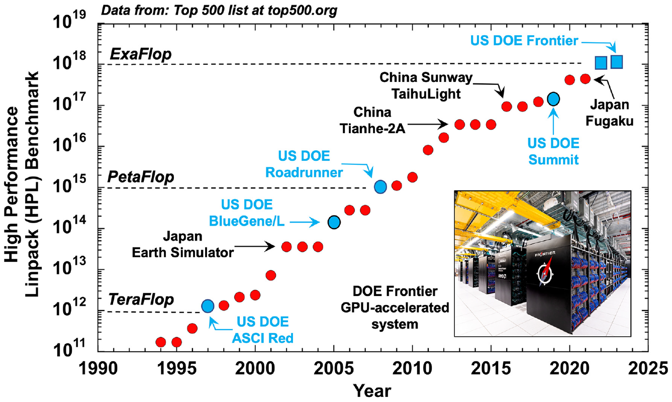
Evolution of the world’s top ranked scientific computing platform through November 2023 as determined by Top500.org (https://www.top500/2023/11/highs/).
Concurrent with the exaflop computer hardware developments, the DOE Exascale Computing Project (ECP) has focused on the creation of software technologies (STs) and advanced scientific applications to exploit these new platforms. The ST component of the ECP project has developed and integrated a software stack to support achievement of the full potential of GPU-accelerated exascale systems. This has included approximately 70 projects spanning programming models, software performance analysis tools, math libraries, data handling (massive I/O), and visualization. In addition, the ECP has supported the development of 24 diverse Application Development (AD) projects spanning a breadth of science and engineering applications (Alexander et al., 2020). The intent of the ECP is to have these applications, each taking advantage of the software technology developments, fully prepared to exploit the new exascale platforms coming online.
To allow computational resource integration in the exascale ecosystem, all DOE GPU-accelerated platforms are linked through the DOE’s high-speed Energy Sciences Network (ESnet) for accessibility as shown in Figure 2. ESnet provides a large fiber optic network backbone with multiple 100–400 Gbits/s optical channels for parallel data transmission. ESNet allows for the transfer of both large experimental data and high-fidelity simulation model output and provides the interconnectivity for optimal utilization of the full suite of exascale computer platform assets in workflow design.
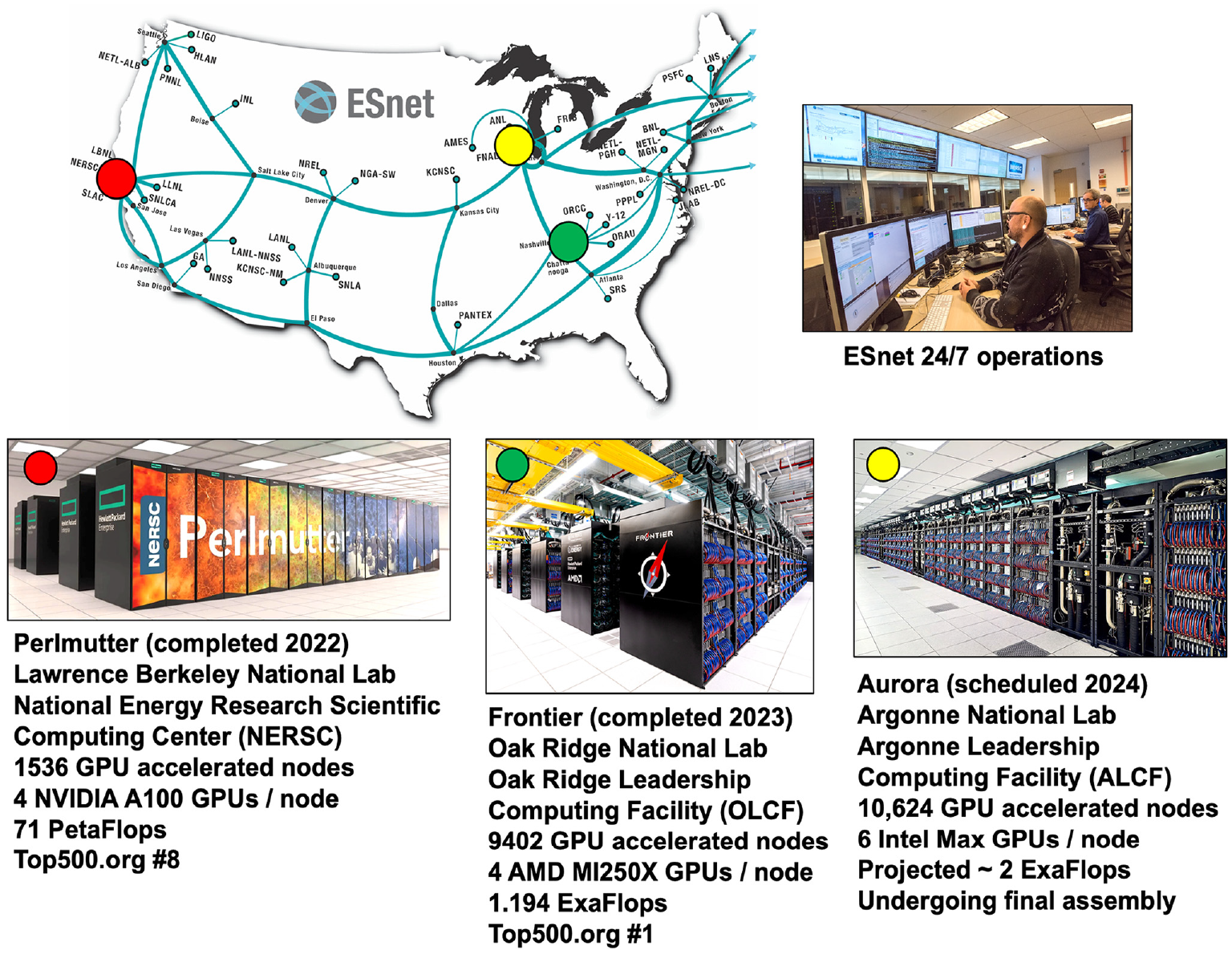
Elements of the DOE Office of Science high-performance computing (HPC) ecosystem; recent GPU-accelerated platforms and site interconnectivity provided by the Energy Sciences Network (ESnet) for high-speed big data transfer.
The EQSIM framework is one of the 24 AD projects and was designed to take full advantage of exascale platforms. EQSIM was designed for seamless execution on all DOE GPU-accelerated platforms and draws upon three key ECP Software Technology applications including:
RAJA—a set of C++ libraries for developing platform-to-platform portability and performance for large-scale scientific software applications on GPU-accelerated systems (Beckingsale et al., 2019);
ExaHDF5—a software library that provides a high-level API with C, C++, Fortran, and Java interfaces for moving data from compute nodes to storage through efficient parallel I/O on exascale computing systems (Byna et al., 2020);
ZFP—a software library with C, C++, and Python interfaces for data compression of floating-point arrays (Diffenderfer et al., 2019; Lindstrom, 2014).
EQSIM utilizes the RAJA libraries to minimize the need for platform-specific code modifications of computational inner-loops when porting across multiple GPU platforms, ExaHDF5 for parallel I/O of massive ground motion data, and ZFP for data compression in very large simulation data sets. HDF5 and ZFP are used in an integrated fashion for on-the-fly asynchronous parallel data output concurrent with ongoing physics computations. The practical benefits of RAJA in terms of portability are substantial and extensive testing has shown that RAJA adds less than 5% computational overhead for all kernel tests.
Over the 7-year duration of the DOE ECP, each of the exascale AD projects were required to establish a DOE approved metric to consistently and quantitatively track advancements in computational performance. To establish regional-scale simulation performance, the EQSIM project utilized the SFBA region of Northern California as a representative regional-scale numerical simulation testbed as shown in Figure 3. To provide a consistent basis for tracking simulation performance, a baseline regional model was constructed for a domain of 120 × 80 × 30 km, and within this regional model, simulations were performed for M7 Hayward fault rupture realizations. The workflow developments and corresponding performance tests summarized in this article are in reference to this regional domain and the existing geophysical data for the SFBA.
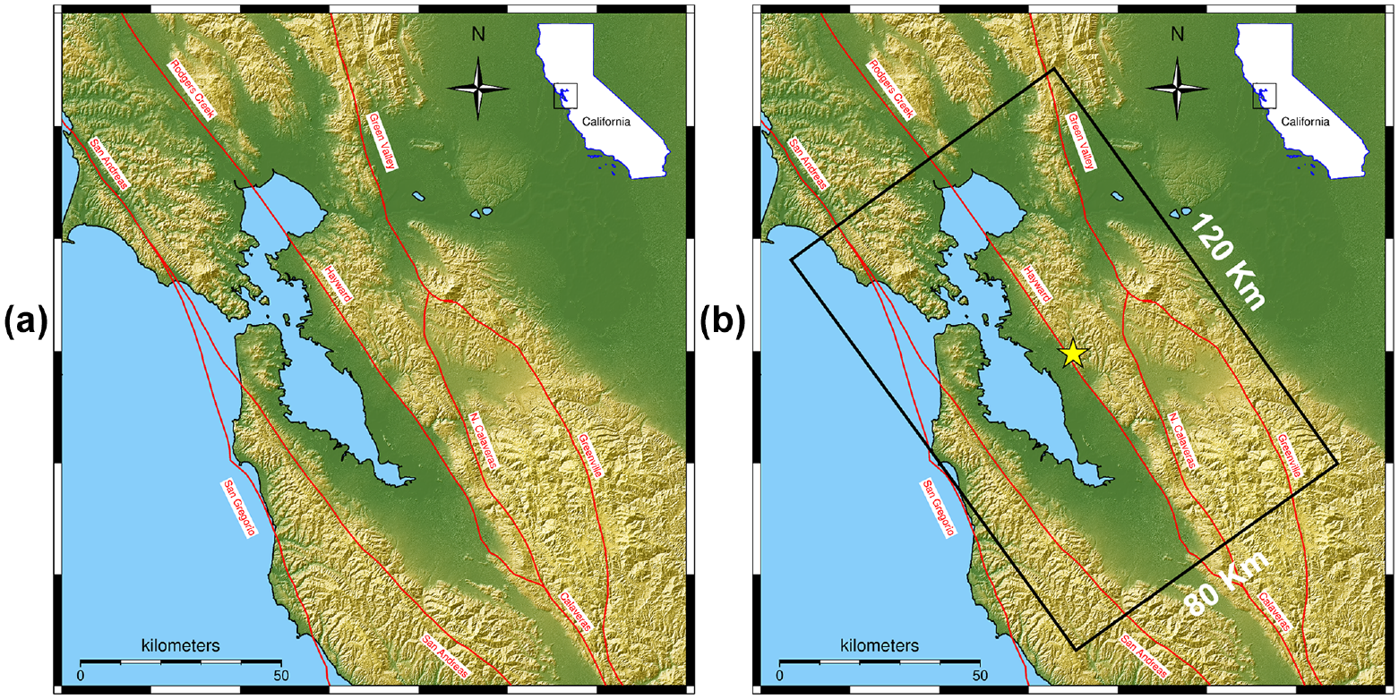
The SFBA region of northern California: (a) SFBA region and major earthquake faults; (b) the black rectangular box indicates the extent of the SFBA regional geophysics model employed in the EQSIM application development (120 × 80 × 30 km).
Maturation of computational workflow for fault-to-structure simulations on exascale systems
When executing regional simulations at hundreds of billions of grid points, any poorly designed and inefficient elements of the workflow are immediately apparent and prohibitive in terms of successful achievement of efficient regional simulations. It is essential that all elements of the workflow are designed and verified by experiential learning from platform-specific performance testing. The overall EQSIM workflow has undergone careful design and extensive development and verification testing to achieve both efficiency and performance on massively parallel GPU-accelerated platforms.
The matured EQSIM fault-to-structure regional simulation workflow is partitioned into three distinct sequential components as indicated in Figure 4. Component 1 consists of three-dimensional simulations of ground motions at regional scale, component 2 consists of evaluation of infrastructure response to the simulated ground motions, and component 3 consists of an interactive visualization and data interrogation capability for efficient inspection and analysis of very large simulation data sets. Each simulation component accesses the right-sized GPU-accelerated platform with the regional-scale ground motion simulations performed on exaflop systems (Figure 4a), the infrastructure response simulations typically performed on pre-exascale high-performance GPU systems (Figure 4b), and data visualization and display performed on a dedicated server system purpose-built for big data manipulation and visualization (Figure 4c).
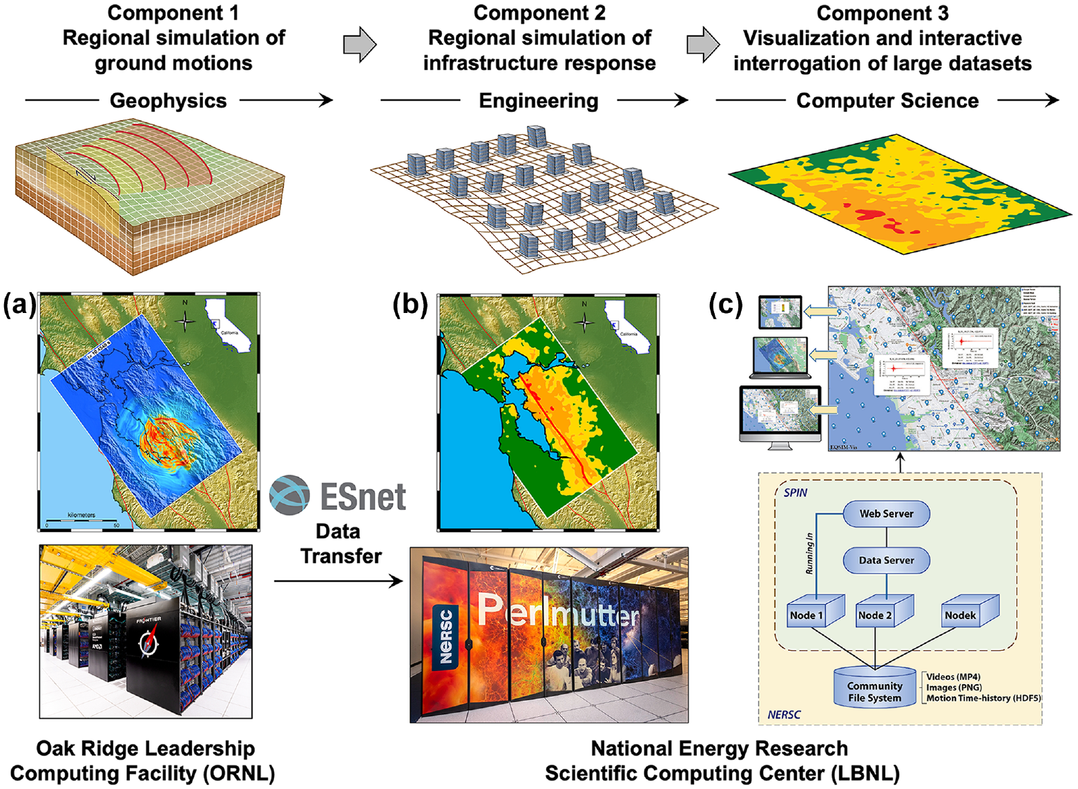
Three sequential components of the EQSIM regional-scale, fault-to-structure earthquake simulation workflow: (a) ground motion simulation; (b) infrastructure response simulation; (c) interactive visualization and display of large regional data sets with EQSIM-vis, components interconnected via the ESnet high-speed network.
An efficient capability for inspecting and mining very large regional simulation data sets is essential for extracting new insight from regional simulations. As described in a subsequent section, the visualization and inspection of simulation data for both ground motions and infrastructure response are performed using the interactive EQSIM-vis software on the dedicated Spin data server at Lawrence Berkeley National Laboratory (LBNL) (Blaschke et al.) which was developed specifically for real-time large data interrogation and display (Figure 4c). The three EQSIM workflow components are now interconnected via the ESnet network which allows rapid and authenticated transmission of hundreds of terabytes to petabytes of data between the various DOE computer platforms and sites.
Workflow component 1
When creating geophysics code input files with hundreds of billions of zones, it is impractical to have multiple fully assembled input files stored on disk as a single input file can easily reach 200+ terabytes in size. In the first step of the EQSIM component 1 workflow, shown in Figure 5, the large regional model input required for the SW4 geophysics code is generated and populated in computer memory, including geologic properties and the fault rupture characterization, at run time. In the most recent instance of EQSIM workflow, the user creation of a minimalist input command file is organized around a construct of efficiently accessing existing large databases for the geologic structure and fault rupture characterization with automated mapping of the geologic data and fault rupture model onto the computational grid.
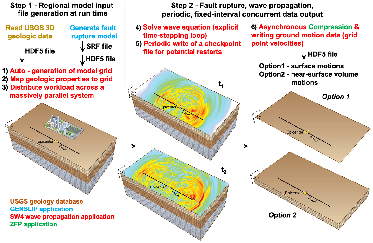
Component 1 of the EQSIM exascale workflow—two steps of the ground motion simulations.
The grid for the regional geophysics model is based on a set of user-defined commands which include user specifications to refine the grid dimensions as a function of depth for both the curvilinear (near-surface topography conforming grid) and Cartesian (at depth computationally efficient regular grid) portions of the SW4 grid. The grid refinement scheme sizes the grid zones to efficiently match the natural depth variation of the geologic properties as illustrated in Figure 6. The grid dimensions are sized to achieve numerical accuracy by employing eight grid zones per the shortest wavelength being resolved, which is dictated by the highest frequency resolution of the simulation being executed, and grid spacing increases with depth to reflect the stiffer materials and corresponding longer wavelengths. The grid refinement finite difference stencils have been developed to ensure maintenance of the inherent fourth-order accuracy of SW4 in space and time (Zhang et al., 2021a). An additional complication is created by the fact that the grid refinements must also be appropriately implemented across the length and width of the surface defining the fault rupture plane and the fault rupture model. The grid at the ground surface is automatically mapped to the surface topography based on an existing database of regional topography.
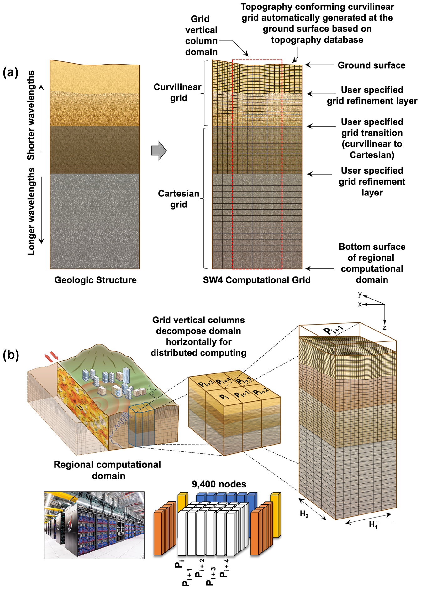
Computational grid generation at run time and distribution of computational effort by grid column partition for massively distributed systems: (a) grid definition and refinement with depth and (b) domain partition to nodes on an Exascale platform.
Once the grid point locations are autogenerated, the geologic properties from the 3D USGS geologic database for the SFBA, stored in an HDF5 container at 100 m horizontal and 25 m vertical spacing (Aagaard and Hirakawa, 2021; Byna et al., 2020) are automatically mapped onto the computational grid based on the grid point spatial location and interpolation of the USGS data. For massively parallel computations, the model grid is distributed across platform nodes using a Message Passage Interface (MPI) library through subdivision of the overall domain into a series of vertical “columns” extending from the lower boundary of the model domain to the ground surface as shown in Figure 6. The column dimensions, H1 and H2 in Figure 6b, are selected to create a grid volume that will distribute the domain of “N” columns to the “N” processors resident on one compute node of the GPU-accelerated platform, that is, one column domain to one GPU. The resultant column domain chunk size is thus dependent on the model depth, the frequency resolution of the simulation, the lowest shear wave velocity resolved in the near-surface layers (mesh spatial density), and the memory capacity of an individual compute node GPU.
EQSIM employs the Graves-Pitarka kinematic fault rupture model (Graves and Pitarka, 2015; Pitarka et al., 2022) and the definition of a fault rupture realization for a specific earthquake is generated through the execution of the stochastic rupture generator routine GENSLIP which creates an SRF text file for the event rupture definition. The SRF text file allows user inspection and checking of the resulting rupture model; however, for large magnitude earthquakes, the SRF is a very large file and computationally inefficient to read into the SW4 code. Consequently, the SRF file defining the fault rupture is converted into an HDF5 data container file with binary data format, resulting, for example, in a speed-up of the file read on the order of 10× for the 1,440,000 sources required for representation of a 10-Hz Hayward fault rupture model input. As the EQSIM workflow has matured and become operationally refined for GPU systems, the model initiation has been substantially automated leading to a very concise and efficient run time command file as shown in Figure 7. Such a file allows expedient multiple runs for the execution of parametric variations, for example, in the analyses of multiple fault rupture realizations for a specific scenario earthquake.
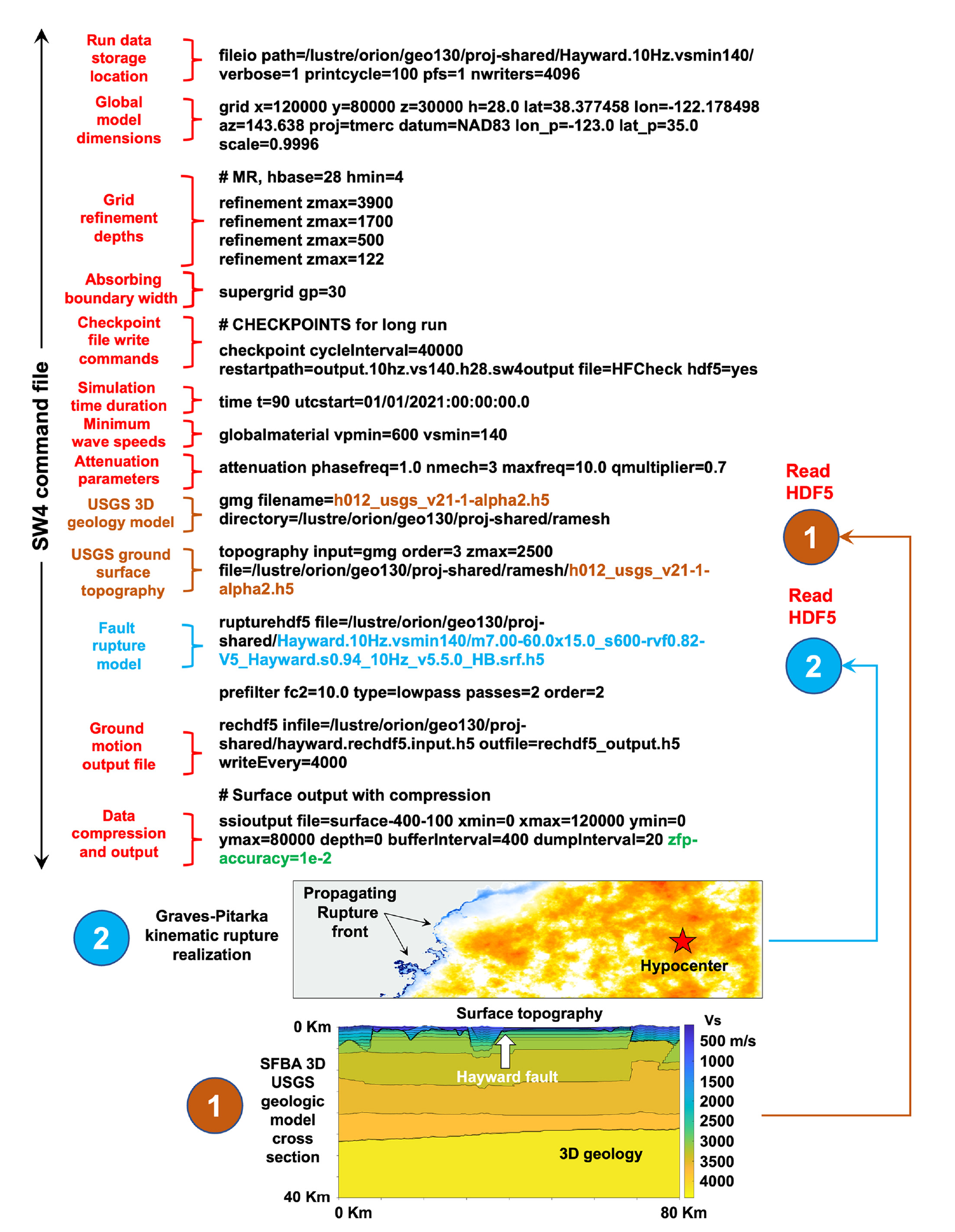
A complete SW4 run time command file for an M7 Hayward fault earthquake simulation for one fault rupture realization.
The second step of the ground motion simulation workflow, which constitutes the bulk of the computational effort for a regional simulation, consists of the time-stepping loop which solves the wave equation over the time duration from fault rupture initiation until the end of the earthquake. The SW4 geophysics code utilizes an explicit, fourth-order predictor–corrector time-stepping algorithm (Petersson and Sjogreen, 2012). As regional model sizes exponentially increase, the computational domain is distributed across thousands of compute nodes and the probability of a computer node fault during time stepping can also increase. To guard against a potential node failure or other hardware fault, SW4 writes periodic checkpoint files at a user-specified interval so that a restart of the earthquake simulation from a previous equilibrium state can be executed in the event a hardware or software failure terminates a large simulation. The new file system on the Frontier exascale platform enables extremely fast checkpoint file creation, for example on the Frontier system using 5000 nodes, parallel data write speeds of up to 4.5 TB/s are realized. The user selection of the frequency for checkpoint file creation is informed by the statistics of the mean time to failure for nodes on a specific massively parallel platform and the data file system write speed.
The second step of the component 1 workflow also includes the output of simulated ground motions. There are two options for the output—one includes the output of ground motions at the surface grid points and the second consists of output for all grid points in a near-surface volume defined by the user. Each output type provides an option for the user to down-sample data to sites with a larger spacing than the model grid point spacing as a data economization procedure. To provide efficient data writes and further reduce the size of generated data, the fundamental geophysics data consisting of three component velocities at each grid point is compressed using the ZFP software library (Lindstrom, 2014). ZFP exploits the fact that the floating-point numerical values of close neighbor grid point ground velocities often have numerically similar values in terms of the numerical elements of both the mantissa and exponent. This provides a data compression principal through the elimination of repeated near-equal numerical values across the large number of grid points.
The initial grid partition strategy illustrated in Figure 6 defines the starting point of the workflow approach to selecting optimal computational work distribution on GPU platforms. For a given regional simulation (e.g. an M7 Hayward fault earthquake in the SFBA), the partition in Figure 6 defines the initial distribution of work. When many realizations of a given earthquake rupture scenario are to be executed, it is essential to identify the strong scaling performance with the number of nodes employed to inform decisions on optimal utilization of GPU platforms. The execution of short duration run scaling tests provides a template for scaling decision-making. Figure 8, for example, illustrates scaling analysis for an SFBA M7 Hayward fault earthquake for 10 and 15 Hz solutions. The initial model for this Fmax of 10 Hz, Vsmin of 250 m/s simulation with 222 billion grid points can fit on 286 nodes of Frontier based on the initial model sizing defined in Figure 6. Strong scaling tests with increasing number of nodes toward full machine usage are shown in Figure 8. This curve illustrates the ability to reduce solution wall clock time from 55.6 to 10.2 h with increased distribution of the problem to the utilization of 2288 nodes, and to 6.3 h with the distribution to 9152 nodes of essentially the full machine. The information in these curves, when convolved with the Frontier computer site operation protocols on user allocated bank time limits and queuing priorities, allows informed decisions on optimal Frontier usage for large regional simulations.
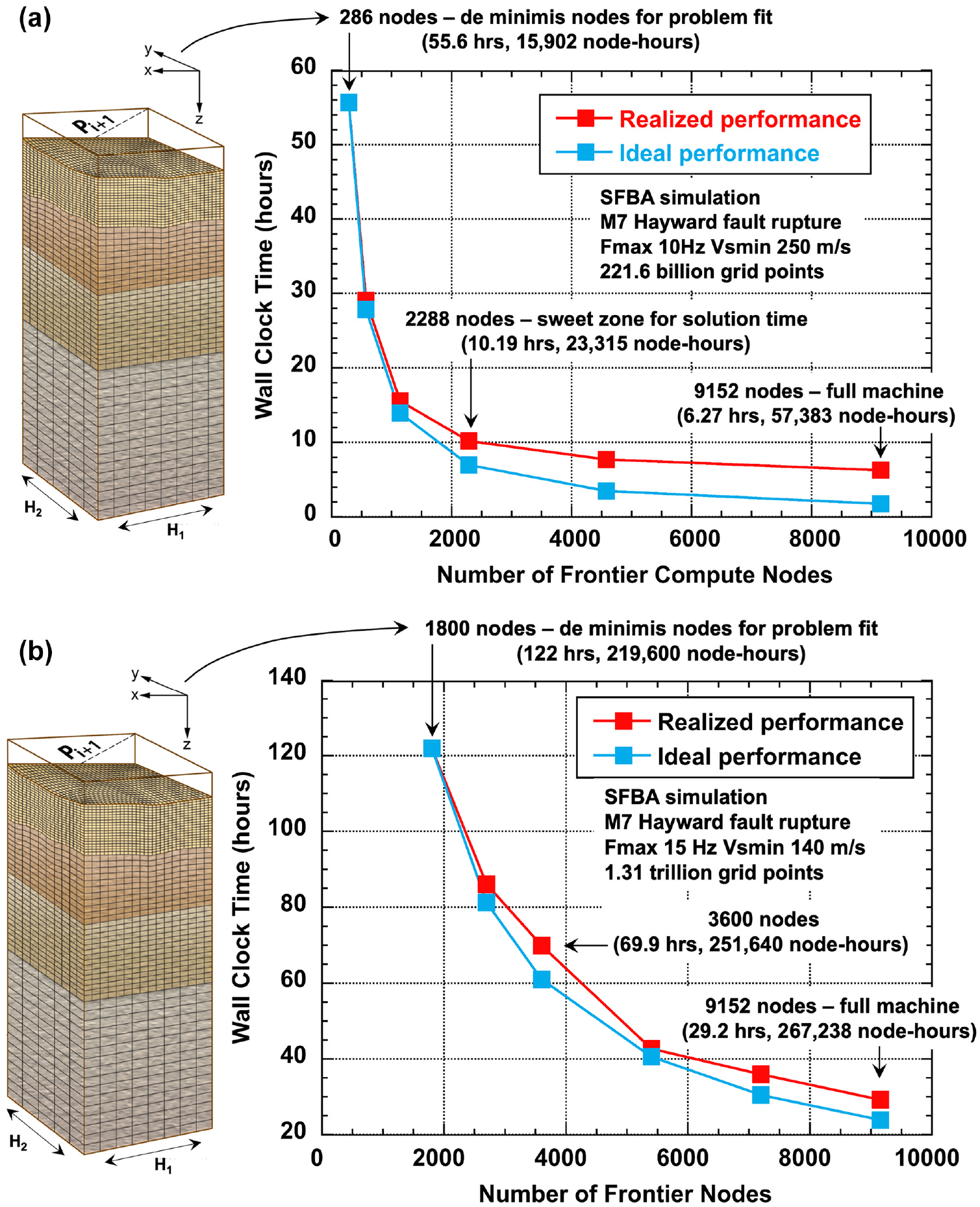
Ground motion simulation scaling example on Frontier: (a) realized strong scaling for a 10-Hz, Vsmin 250 m/s 221 billion grid point SFBA simulation; (b) realized strong scaling for a 15-Hz, Vsmin 140 m/s 1.31 trillion grid point SFBA simulation.
A representative massively parallel regional ground motion simulation must harmonize the EQSIM workflow with the queuing and job limit protocols of the specific computing facility where computations are being executed. For the new Frontier exascale system, there is a wall clock run time limit of 12 h for any single run, and the system assigns higher queue priority to jobs that utilize a larger portion of the machine nodes. Balancing the workflow and supercomputing facility requirements, a representative large ground motion simulation is shown schematically in Figure 9. The job start-up described in the component 1 workflow typically takes on the order of 25 min after which time stepping initiates, given the newness of the Frontier platform and the potential for node faults, checkpoint files are currently written in approximately 2-h intervals. During a checkpoint write, the time stepping is paused for a very short duration (tens of seconds) to complete the checkpoint output. This short duration of pause is facilitated by the efficiency and speed of the exascale file system. Based on experience gained from numerical testing, ground motion output is buffered for 400–800 time steps and then written asynchronously by an available idle CPU concurrent with ongoing GPU computations. Extensive numerical testing has informed data chunk size for achieving optimal write times (Tang et al., 2021). Given the current limitations on Frontier job run times, large earthquake simulation time stepping must be dividing into 12 h segments as shown in Figure 9.
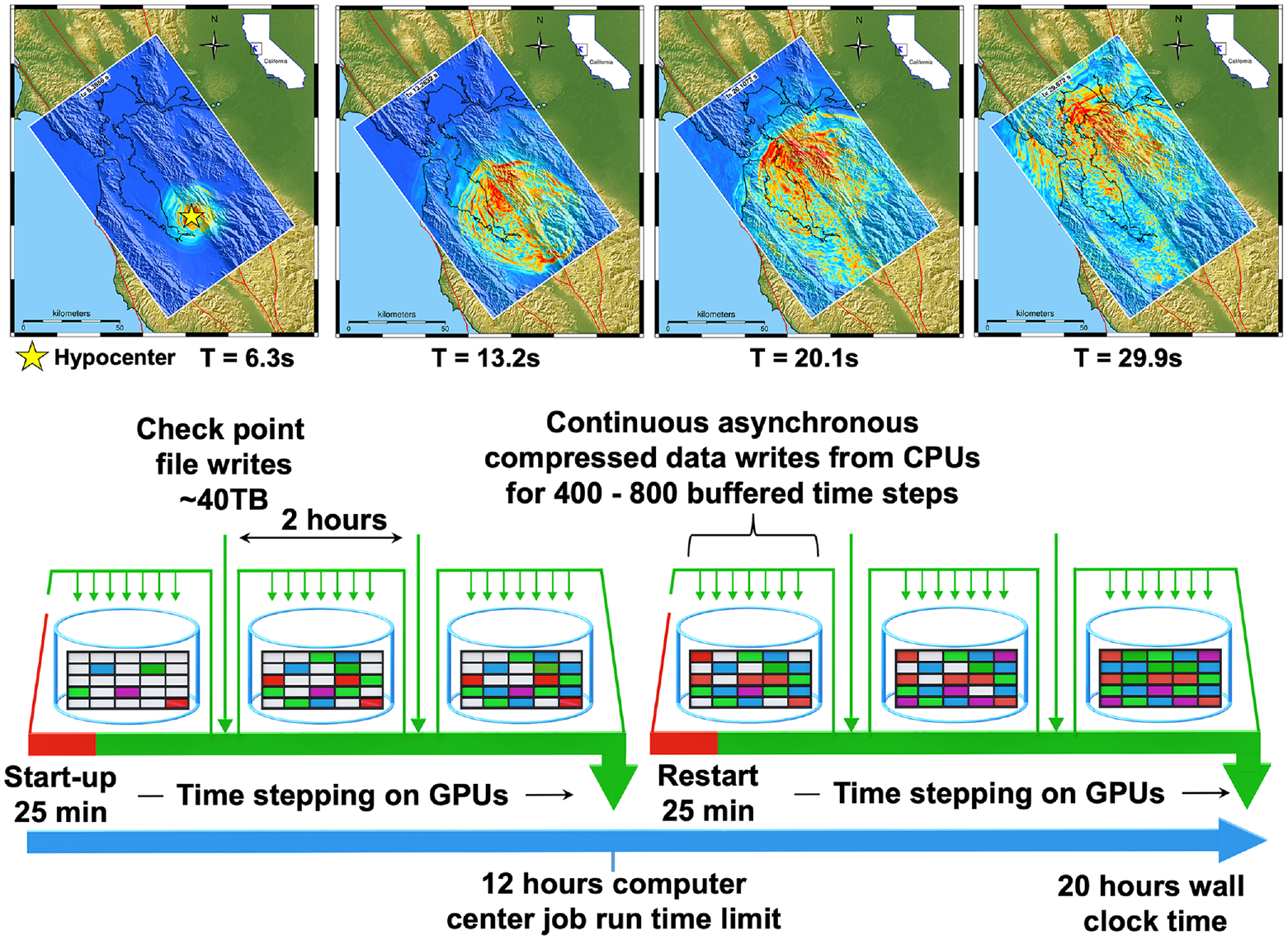
Anatomy of a massively parallel regional ground motion simulation on Frontier (Fmax 10 Hz, Vsmin 250 m/s, 221 billion grid point simulation of an M7 Hayward fault rupture).
Workflow component 2
Component 2 of the EQSIM workflow consists of simulation of the seismic response of infrastructure systems with the three steps shown in Figure 10. Step 1 consists of appropriate ground motion assembly for the problem at hand. Two workflow options are incorporated for the coupling of the regional geophysics and local engineering models as shown in Figure 10. The first, indicated as Option 1, utilizes the simulated horizontal and vertical ground motions at a point on the ground surface applied uniformly across the base of a structure of interest to define the support motion in a fixed base analysis. This approach neglects any effects of soil–structure interaction and does not account for the potential spatial variation of motions that can be generated by inclined body- and surface-waves across the footprint of the structure. It is noted that this approach can also allow inclusion of the simulated site ground surface rotations as part of the infrastructure forcing function. The ground rotations can be obtained by differencing the vertical ground displacements over a selected horizontal gauge distance (Wu et al., 2021). The second workflow option utilizes a DRM boundary to rigorously transfer the surface tractions from the geophysics model to the soil island boundaries in a local engineering soil/structure model as indicated in step 2 of Figure 10. This second workflow allows full representation of soil–structure interaction and fully honors the complex incident wavefield that includes inclined body waves and surface waves. These two coupling representations, referred to as fixed base and fully coupled respectively, provide user options for infrastructure response simulations and allow critical evaluation of traditional engineering process models (McCallen et al., 2022; Wu et al., 2020, 2021). In the EQSIM workflow, multiple engineering codes have been successfully linked to the SW4 geophysics model through DRM coupling including Nevada (McCallen and Larsen, 2003), OpenSees (McKenna, 2011), and LS-DYNA (Livermore Software Technology Corporation (LSTC), 2021).
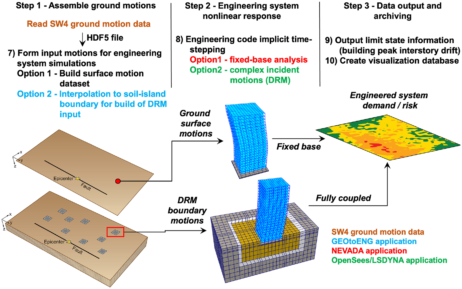
Component 2 of the EQSIM exascale workflow—infrastructure response simulation.
The second step of the workflow includes the response history time-stepping solutions for the infrastructure systems, which in the EQSIM workflow is performed using implicit time integration nonlinear finite element representations. For cases where an archetype building structure is being analyzed across the entire domain surface using the fixed base option to develop an understanding of the regional distribution of risk, the computational effort is efficiently distributed through a naive parallelization in which each building simulation is assigned to an individual processor.
For the strongly coupled case, in which the DRM is used to couple the regional geophysics model to the local engineering model soil–structure island, a ground motion interpolation algorithm and associated processing software have been developed to efficiently compute the motions on an arbitrarily oriented DRM boundary. To apply a DRM boundary for any location in the regional domain requires that the data for a given earthquake realization be saved in Option 2 format where grid point velocity data is stored for a user-specified near-surface 3D domain volume as shown Figure 5. As the model global horizontal dimensions are defined by the region under consideration, the user simply provides a depth to which the grid point data will be saved so the data volume is sufficient to contain the structure-soil system or near-surface soil layer of interest. Given the extreme size of the geophysics grid, it is essential to employ an efficient algorithm for locating the DRM boundary and extracting the required boundary motions as the option 2 data set can contain billions of grid points. In recent work, this approach has been generalized to allow easy application to any engineering code that has implemented the DRM. The first step of the coupling consists of translating the local engineering model coordinate system into the global SW4 coordinate system as shown in Figure 11a. Next, the user specifies the global model coordinate location of the centroid of the engineering model grid, the horizontal angle of the engineering soil domain relative to the global geophysics model axes, and the dimensions of the engineering soil island, D1 and D2, as indicated in Figure 11. A developed Python-based code “GEOtoENG” then computes a 3D bounding box for the geophysics grid just large enough to encompass the engineering model domain as indicated in Figure 11. This constrains the consideration of grid point data to a very small subdomain in the large option 2 data set. Once the bounding box is established, GEOtoENG creates a continuous velocity field within the bounding box by employing a spline-function to interpolate the discrete velocities from the geophysics code grid points based on the general approach outlined in McCallen et al. (2022). The velocities at the DRM boundary are then computed from the continuous velocity field within the bounding box based on the global coordinates of the engineering domain grid points. Once DRM boundary velocities are determined, the DRM nodal accelerations and displacements required for the engineering code DRM boundary are used to generate an input file for the local engineering code earthquake simulation. For the EQSIM framework there are two principal use cases that the DRM implementation is intended to support, in the first case, the DRM is utilized to couple a local structure/soil island model to the regional geophysics model to capture the combined effects of soil–structure interaction and the system response to complex inclined incident body waves and surface waves as shown Figure 12. In the second use case, the DRM bounds a near-surface geotechnical layer where a nonlinear model can be employed to represent the shallow soil response as shown in Figure 12. Current EQSIM work is focused on implementation of an equivalent linear representation of nonlinear soil and testing of the DRM performance for a localized nonlinear domain.
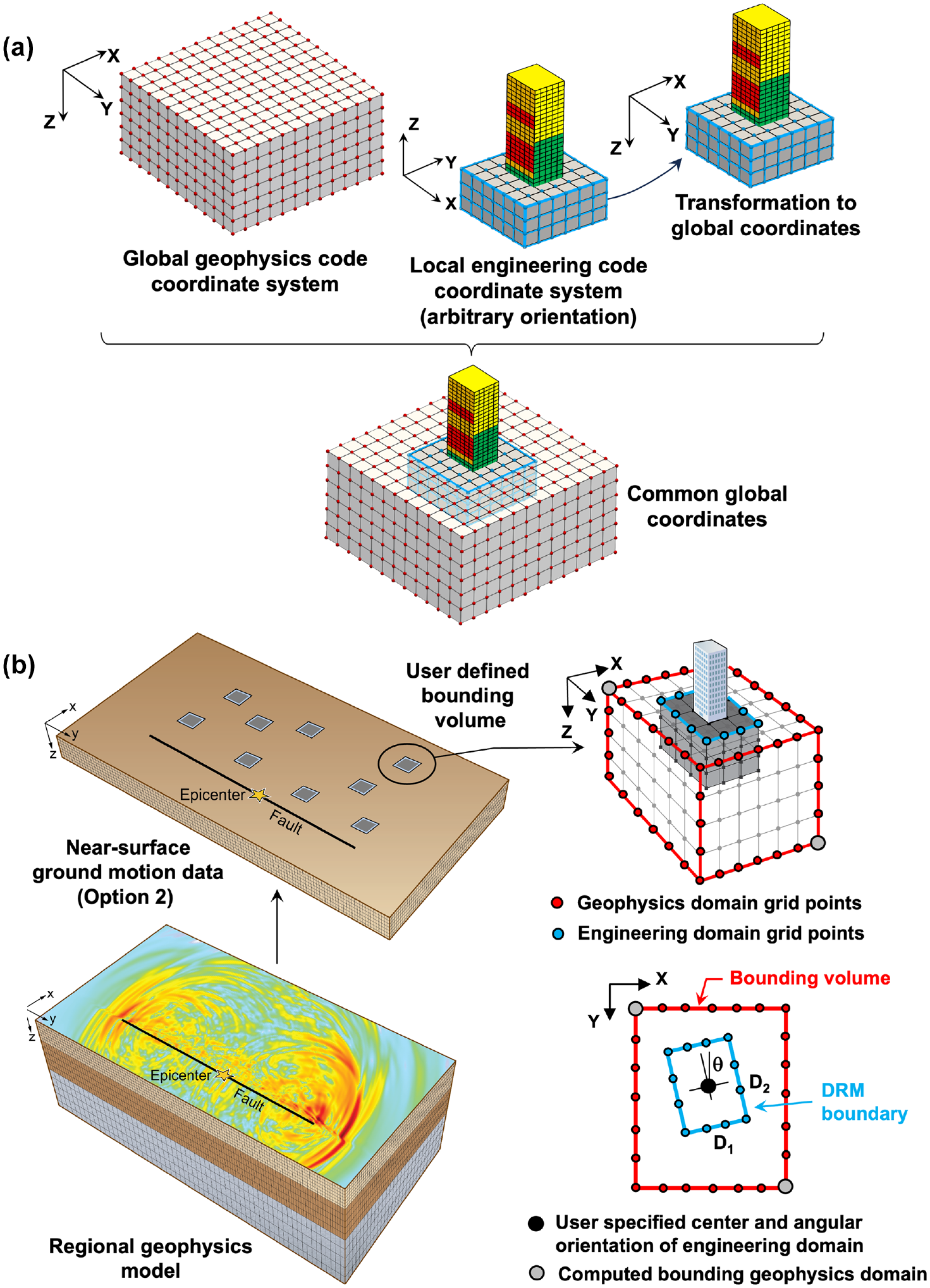
GEOtoENG workflow for DRM coupling of regional geophysics with local engineering models: (a) translation of the local engineering model coordinates into global coordinates; (b) specification of the DRM location in the global geophysics model and autogeneration of a bounding box in the geophysics model grid.
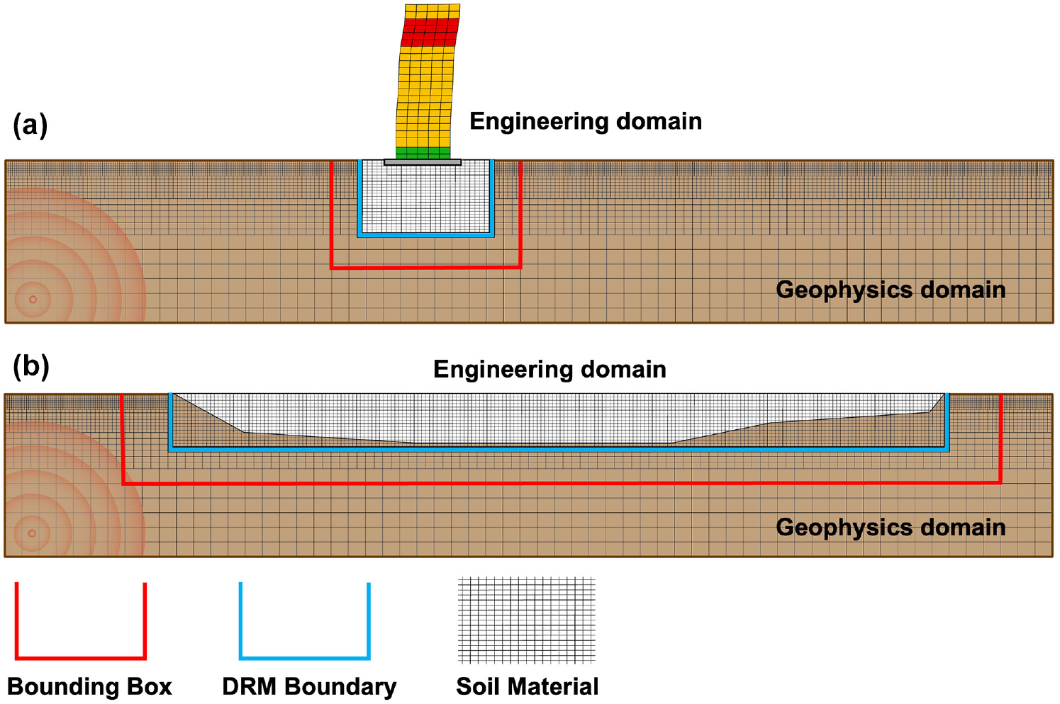
Planned use cases for the DRM in the EQSIM framework: (a) coupling regional geophysics and local structure–soil island models and (b) representation of a near-surface nonlinear geotechnical layer.
The step 3 final element of the workflow includes the output of infrastructure response data. In the case of regional-scale simulations, there is a very large volume of distributed infrastructure response data which must be inspected to gain insight into the spatial distribution of infrastructure demand and one element includes visualization of building demands as shown in Figure 13. To achieve optimal visualization efficiency and flexibility in the visualization engine, the eXtensible Data Model and Format (XDMF), which is designed to exchange data between HPC codes, is adopted (XDMF, 2017). Within this data scheme, a text-based XML file stores light metadata describing the structure of the data sets for the computational finite element mesh while the heavy data including the nodal locations, element connectivity, and various structural responses of interest are managed in an array-oriented HDF5 database that supports fast random parallel access during the rendering stage.
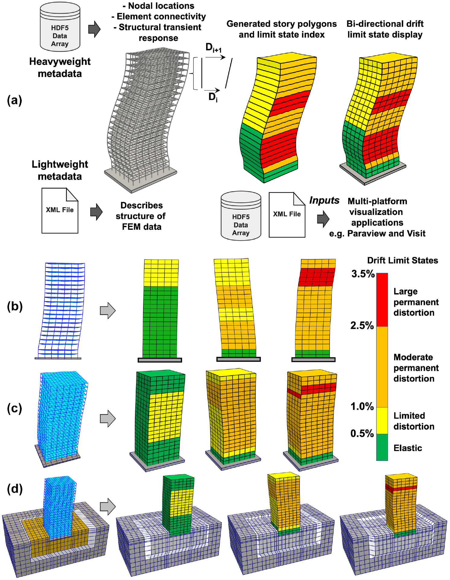
Visual animation of building deformations and color-coded peak interstory drift limit states achieved during earthquake motions for 2D and 3D steel moment frame building system models (ASCE 43-19 drift limits): (a) developing a generalized approach to nonlinear building response visualization using HDF5 and XML data sets; (b) planar model (Nevada); (c) three-dimensional model (OpenSees); (d) coupled building soil system model (OpenSees).
The visualization process in the current implementation has been generalized to allow application to multiple engineering codes following two steps. In the first step, building response simulation data is stored inside a compact and extensible HDF5 database. Apart from visualizing the transient nodal and elemental responses which are recorded by the finite element codes, using an extensible HDF5 database provides a flexible framework to allow on-demand incorporation of additional important structural damage measures, for example, the building story drift limit state, for seismic demand visualization. For finite element programs that support outputs in the HDF5 format, this step can be simplified by reusing the existing hierarchical structure of the respective output data files, and efforts can focus on the addition of user-specified structural damage measures that are of interest. In the second step, a descriptive XML file is generated based on the hierarchical structure of the HDF5 database from step 1. To reduce manual intervention in the process, the generation of the XML file is automated through customized Python scripts. The XML description file and its associated HDF5 database allow direct importation into existing multiplatform visualization applications including ParaView (Ahrens et al., 2005) and VisIt (Childs et al., 2012) for image rendering and data analysis. This approach allows common visual renderings to be implemented across a breadth of engineering simulation codes. To provide direct visual interpretation of structural demands and damage potential, animations of building transient response for both 2D and 3D building analyses are output in MP4 format with a color coding associated with specified peak interstory drift (PID) limit states occurring at each building floor over the earthquake duration as shown in Figure 13. This visualization approach enables the efficient inspection of regional-scale building response through an EQSIM-vis interactive web-based browser window as described below.
Workflow component 3
An ultimate objective of regional simulations is to provide the capacity to execute a significant number of simulations that can span the space of model features and parameters that are not well constrained for a particular earthquake scenario. For example, the specific manner by which a given fault will rupture in a future earthquake is not known beforehand, necessitating the inclusion of a suite of rupture realizations that reflect the breadth of possible fault ruptures for risk assessments. One of the principal values of high-fidelity regional simulations is the ability to generate spatially dense ground motions for site-specific evaluations; however, this can result in very large data sets that contain hundreds of terabytes to petabytes of data when stacking a number of rupture realizations. As illustrated in Figure 14, the data storage requirements for an M7 Hayward fault scenario simulation with Fmax = 10 Hz and Vsmin = 140 m/s in the San Francisco Bay Area can be quite large. For ten rupture realizations, the storage of raw simulation data (uncompressed and not spatially down-sampled) for ten Hayward fault rupture realizations is 3.1 petabytes corresponding to ground motions at a 1.75-m grid spacing. It is also noted that this is only considering data at the ground surface (option 1 in Figure 5), if volumetric data associated with option 2 storage is used, this data size could grow by an order of magnitude or more. While this size of data can be stored in the memory of a super computer, it is difficult to effectively access and interactively data-mine such large data sets.
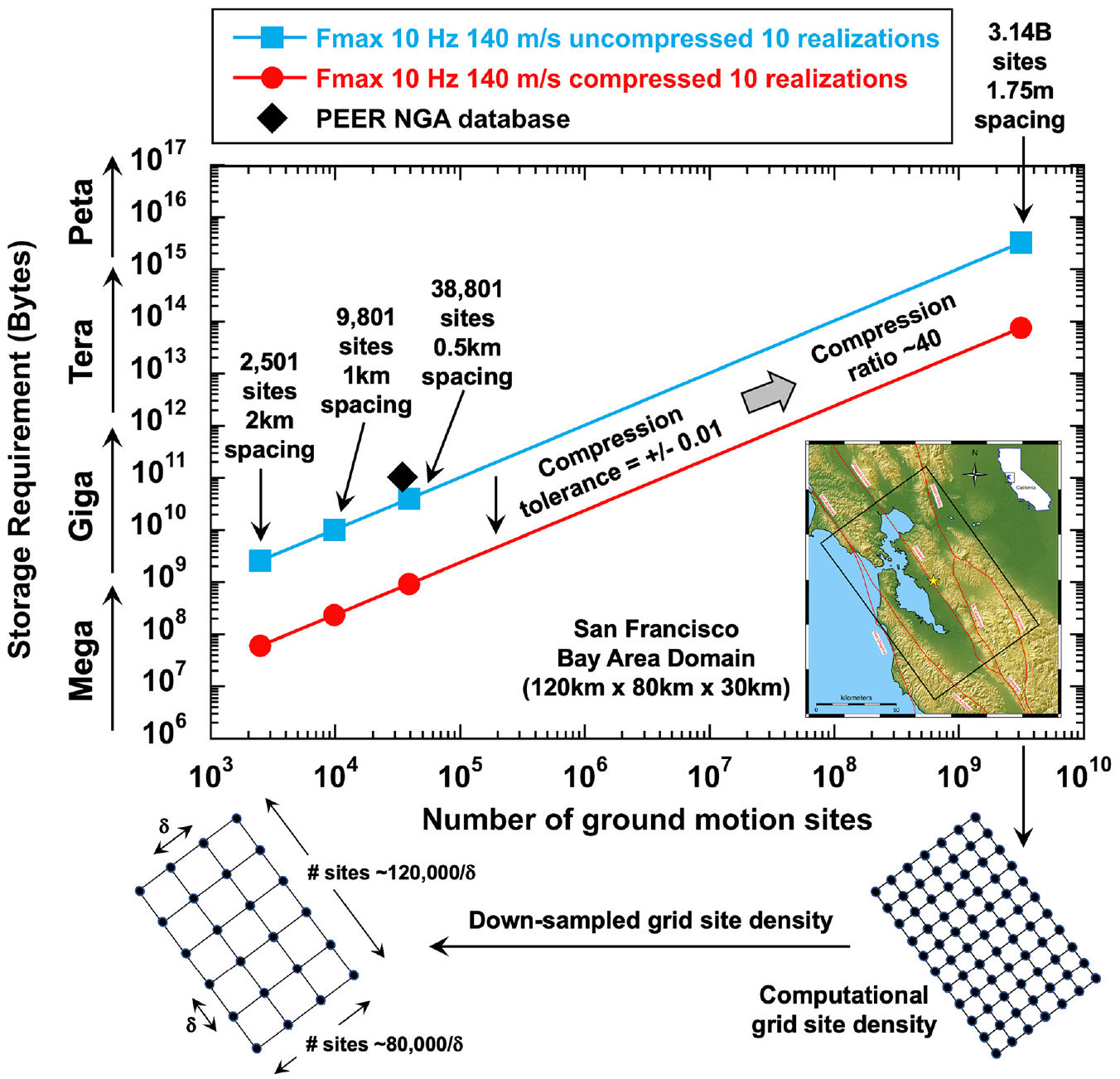
Data storage requirements for a suite of regional-scale simulations (option 1 simulated surface motion data for ten realizations of an M7 Hayward fault event with Fmax = 10 Hz, Vsmin = 140 m/s).
EQSIM has developed multiple features for enabling efficient data manipulation, analysis and exploitation. These options include data compression to reduce the overall data set size and spatial down-sampling to reduce the number of data sites in an operational database. Depending on the application of interest, these data economizing options can be applied to different degrees. Representative reductions achievable in applying data compression and spatial down-sampling are indicated in Figure 14, where a compression factor of approximately 40× can be achieved through ZFP data compression, and for the San Francisco Bay Area, if ground motion data are down-sampled to a spacing of 2 km a data set approximately equal to the existing entire PEER NGA database (94 GB) is obtained for ten Hayward fault rupture realizations. In the EQSIM workflow, either one or both of these options can be selectively employed depending on the desired use of the ground motion database.
Component 3 of the EQSIM workflow, shown in Figure 15, was created to allow efficient interactive visualization and knowledge extraction from the large data sets generated by regional-scale simulations. The workflow for component 3 is developed around the new EQSIM-vis software application for visualization-based searches and selective user download of simulation data. EQSIM-vis exploits the Folium Python package which internally utilizes the leaflet.js library to visualize data on an interactive map, for EQSIM-vis, various Google map options can be used for the resident background. In step 1, data saved from the component 1 ground motion simulations and component 2 building simulations are gathered, these data sets are utilized in preparing visual input for EQSIM-vis.
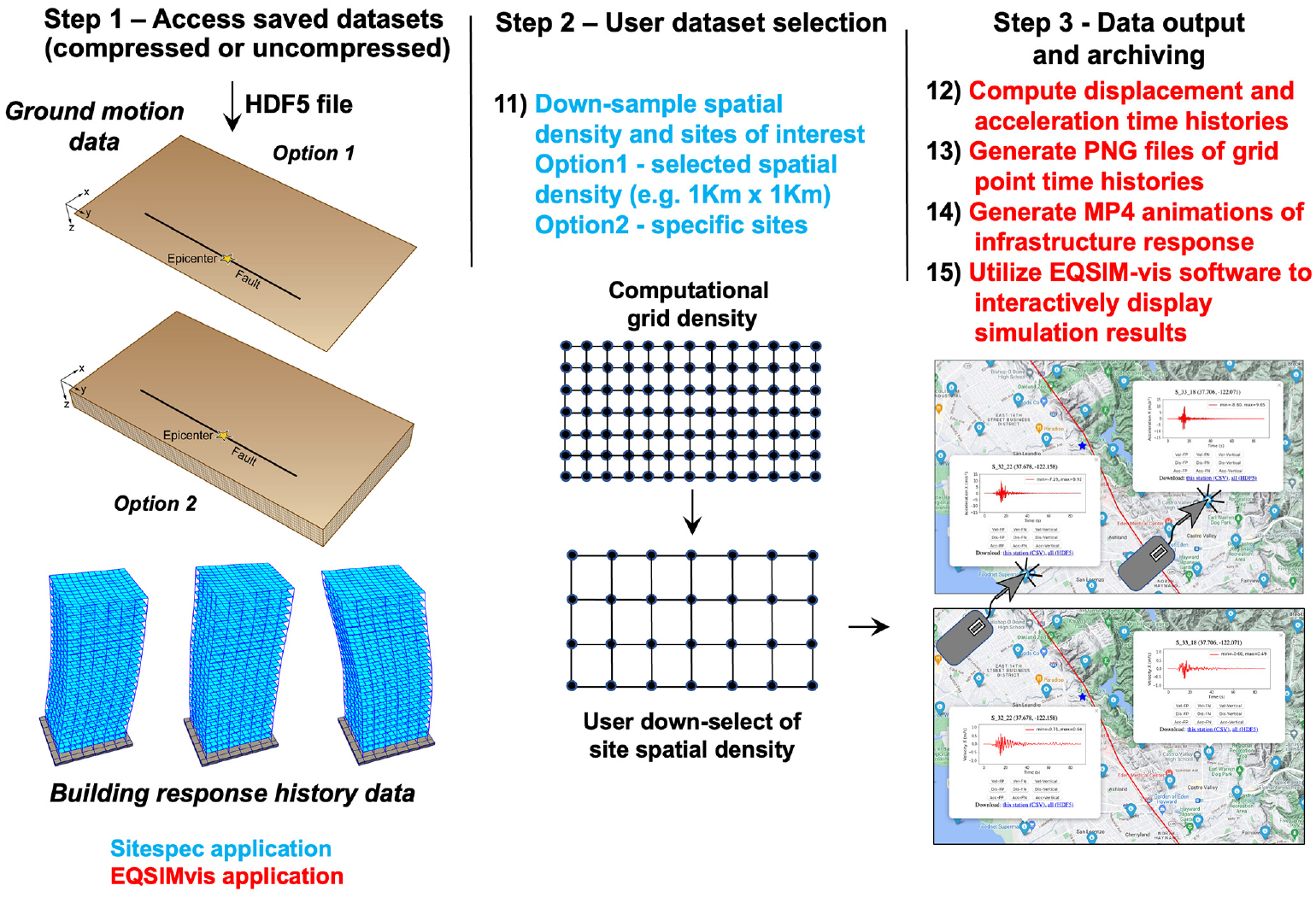
Component 3 of the EQSIM workflow—interactive visual display and browsing of large data sets on the SPIN server with the EQSIM-vis application.
For the regional-scale simulations of the SFBA, two baseline surface ground motion data set options are currently saved for each regional simulation at different spatial resolution. One data set consists of uncompressed grid point velocity data for surface sites at a 2-km spacing yielding 2500 ground motion sites across the SFBA domain and the second data set consists of compressed data for every grid point on the geophysics model surface, which for a Fmax = 10 Hz, Vsmin = 140 m/s simulation gives ground surface motions at a 1.75-m spacing yielding 3.14 billion ground motion sites. Depending on the application at hand, it may be desirable to select a different spatial density for ground motion data and step 2 of the workflow allows for user selected down-sampling of data.
The SPIN server is part of the available computational edge services available at LBNL (Bard et al., 2022), which includes network resources that sit at the edge of the HPC environment and help with the organization and dissemination of HPC simulation results (Blaschke et al., 2021). This server was designed and constructed specifically for managing and efficiently manipulating big-data applications. As shown in Figure 16, SPIN utilizes pre-generated PNG and MP4 files to allow rapid interactive display of both ground motions and structural response. EQSIM-vis is implemented on SPIN to allow user interaction with large regional-scale data sets and to exploit the available interactive data visualization capabilities. Given the large number of PNG and MP4 files associated with a specific regional simulation, these files are pre-processed in parallel and stored on SPIN for a given regional simulation. Once PNG and MP4 files are loaded on the SPIN server for a given event, EQSIM-vis provides agile interactive access to the full data set for a specific earthquake. The user can move locations and zoom in and out via mouse dragging and clicking on a Google map rendering where ground motion stations are indicated by clickable stickpins on the map interface. EQSIM-vis is currently configured to display a wave propagation animation of the earthquake scenario simulation, contour plots of peak ground acceleration and velocity, ground motion response histories including accelerations, velocities, displacements, and animations of building response including visual representation of building PID limit states as shown in Figure 16. EQSIM-vis can be accessed by any compute platform (desktop, laptop, pad, tablet, smartphone) capable of displaying a Google map.
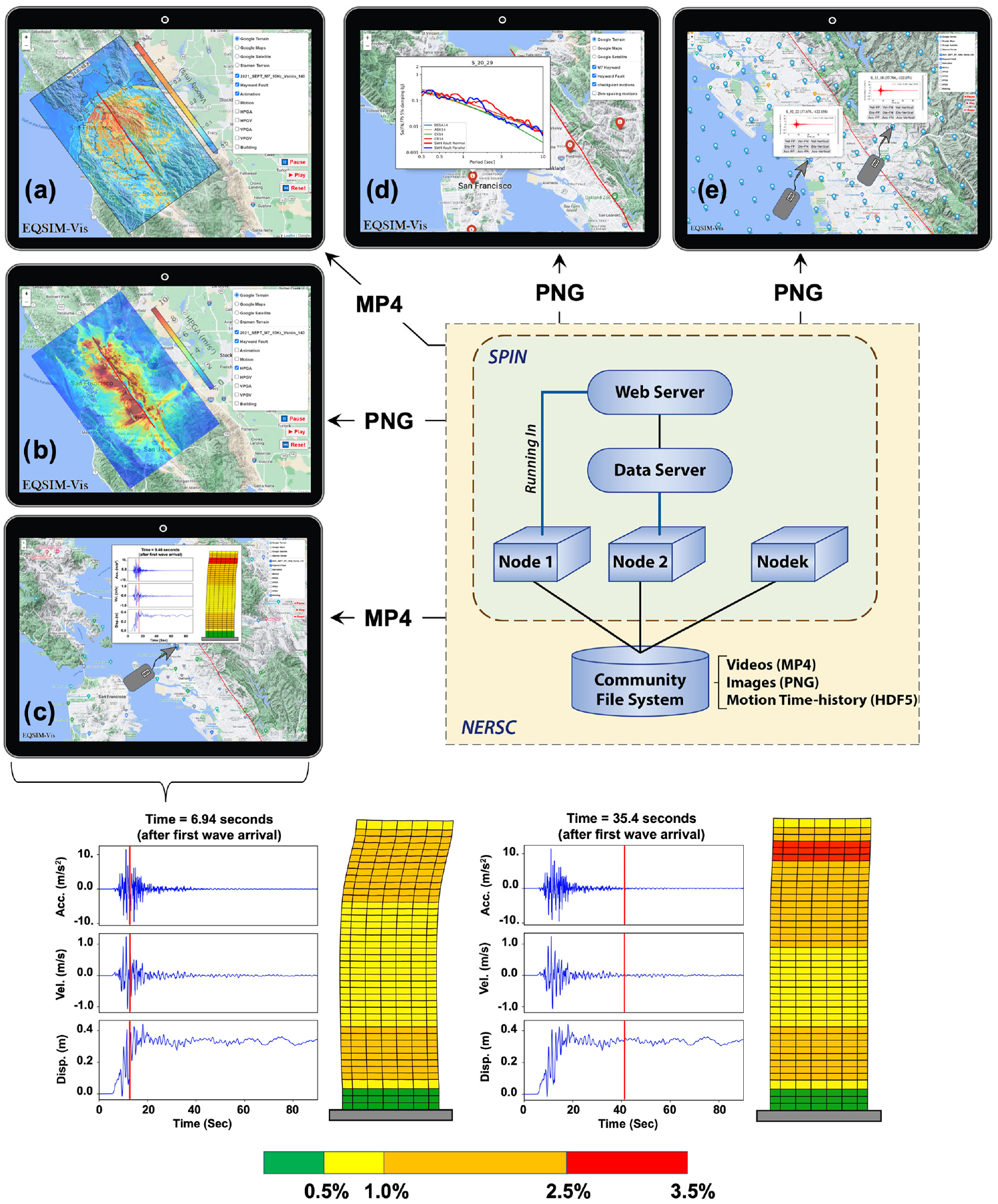
The SPIN data server for visualization, data access, and interrogation based on precomputed PNG and MP4 files for interactive display of regional-scale simulations, visualization options include: (a) rupture animation; (b) ground motion contours; (c) inspection and download of motions; (d) comparison of empirical ground motion prediction models with simulated ground motions; and (e) animation of building response at user selected sites.
Once a particular site is user selected, a PNG file opens for the requested component of ground motion with the click of a mouse as shown in Figure 16. This provides the capability to visually inspect ground motion waveform details for any sites throughout the domain very efficiently. The user can also select a box click to either download the ground motions at the displayed site or an alternative box click to download the displayed component of motion for all sites in the entire computational domain.
Building dynamic response can be viewed in a movie animation at any site location with a view window being opened to display an MP4 animation of the building response. The building response movie includes a dynamic line sweep across the ground motion time series plot (red vertical line in Figure 16) in time synchronization with the building animated response showing the building vibrational shape and the evolving interstory drift limit states occurring at each floor as shown in the two time snapshots. This allows insightful interpretation of the relationship between the ground motion and building response, as well as the time and spatial evolution of building damage. For the 40-story steel moment frame undergoing inelastic response in Figure 16, animation of the results indicates that the building is subjected to higher mode contributions to response that whips the upper floors of the building as a result of the rapid ground surface fling-step occurring fault parallel at this near-fault site. The EQSIM-vis software provides the user an intuitive, simple, and efficient interactive tool for exploring the very large data sets associated with regional simulations and is an essential tool for making high-fidelity regional-scale simulations practical and routine.
Computational performance on GPU-accelerated exascale systems
With the ultimate objectives of computing broad-band, high-fidelity regional earthquake simulations and providing an ability to explore a large suite of scenario earthquake realizations and the full model parameter space, advancing regional simulation computational performance is essential. The progression of performance of the EQSIM workflow and regional simulations was measured with respect to the SFBA region shown in Figure 3. For this regional simulation, the EQSIM application DOE approved Figure of Merit (FOM), which was used to quantify simulation advancement for the ECP performance tracking, was established as:

This expression of the FOM reflects the fact that computational effort varies as the maximum frequency resolved to the fourth power and as the inverse of the minimum ground velocity resolved to the fourth power. The numerical fourth-order dependencies embedded in Equation 1 reflect the computational challenges associated with increasing the frequency resolution of a regional simulation as well as lowering the minimum shear wave cut-off velocity in a regional simulation. In Equation 1, the constant 500 reflects the initial EQSIM SFBA regional simulations performed at the Vsmin cut-off of 500 m/s at the initiation of EQSIM development, and the constant factor of 7.6 was introduced to create an FOM of 1.0 in the first performance runs executed on CPU-based platforms at the start of the EQSIM project in 2017.
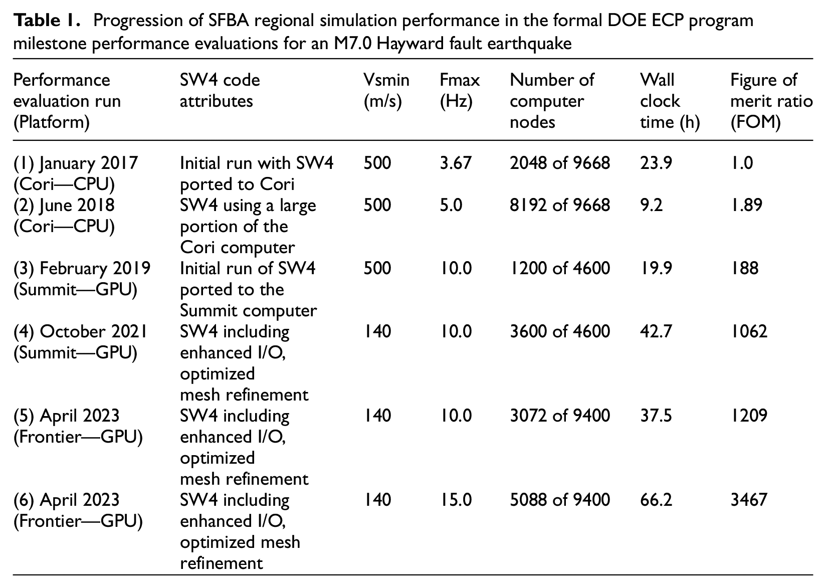
Over the duration of EQSIM development, realized computational performance advancements have resulted from the combined benefits of development and implementation of advanced algorithms, such as the optimized depth-dependent refinement of the computational grid, the previously described advancements in efficient end-to-end workflow and I/O, and the emergence of new GPU-accelerated massively parallel platforms. Table 1 summarizes the key performance milestone tests over the duration of the EQSIM project starting in 2017 through 2023, and Figure 17 graphically illustrates the overall FOM advancements. The FOM ratio in Table 1 and Figure 17 indicates the achieved peak FOM relative to the FOM in the initial SFBA benchmark simulations on CPU-based platforms in 2017. As a requirement of the DOE ECP program, it was necessary to achieve an FOM ratio of at least 50× over the duration of the development project, for EQSIM, the maximum realized ratio was 3467× indicating a very substantial increase in performance.
Progression of SFBA regional simulation performance in the formal DOE ECP program milestone performance evaluations for an M7.0 Hayward fault earthquake
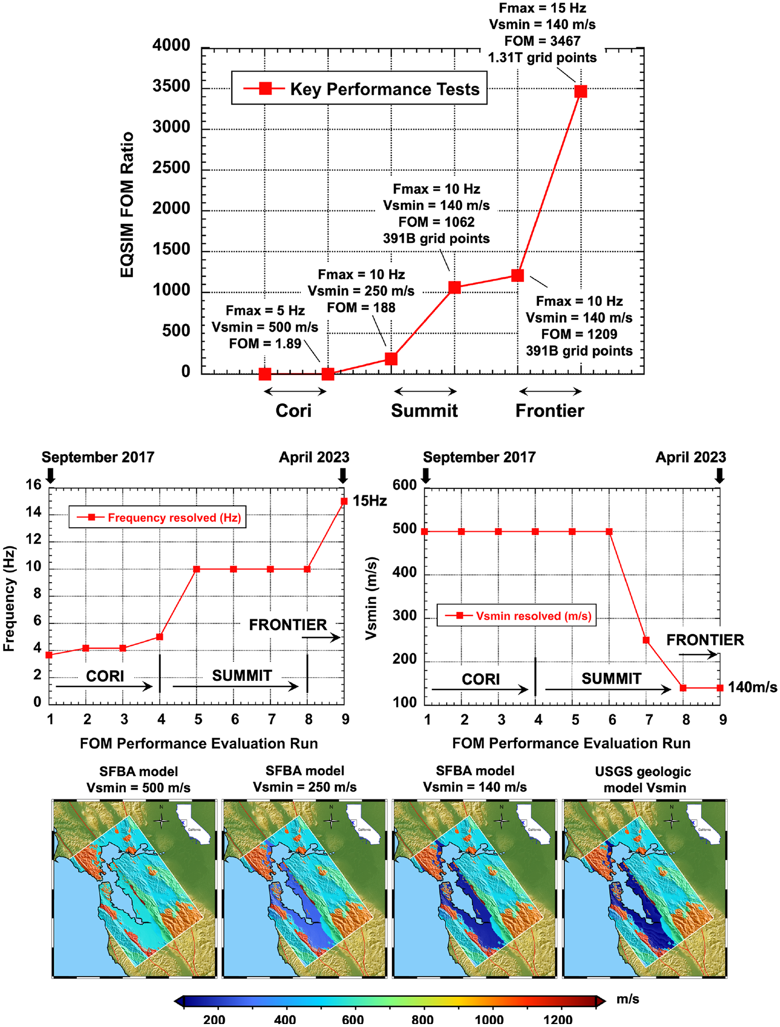
Increases in the EQSIM FOM and frequency and soft sediment resolution over the life of the ECP development project with the transition from CPU (Cori) to Exascale GPU (Frontier) systems.
The EQSIM performance test cases summarized in Table 1 illustrate a progressive increase in frequency resolution in combination with a progressive decrease in the resolved minimum shear wave speed in the near-surface geotechnical layer. This overall progress in regional simulations is further illustrated in Figure 17 where the increase in frequency resolution and representation of soft near-surface sediments is shown graphically. By comparing the near-surface velocity structure resolved by the computational model with the velocity structure in the USGS community model, it is noted that it is necessary to resolve soft sediments with a velocity on the order of 140 m/s to fully honor the geotechnical material velocity in the existing USGS material model for soft sediments around the margins of the San Francisco Bay. These soft sediments underly major urban centers of the east bay and south bay as indicated by the deep purple zone in Figure 17.
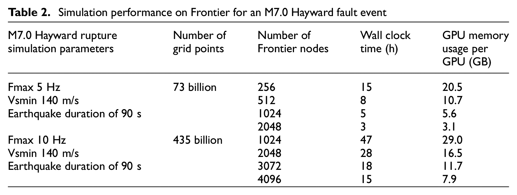
The Frontier exascale system became available for early access and EQSIM performance certification in April 2023 (Table 1), subsequently, as the parallel network and file systems have continued to become more stable and fully production ready, performance has continued to improve. The most recent performance realizations for SFBA simulations of an M 7.0 Hayward fault event are summarized in Table 2. For 5 Hz solutions, which are sufficient for a large population of building structures, a Hayward fault rupture realization can be completed on Frontier in 3 h wall clock time which permits rapid execution of a large number of realizations for the Hayward scenario event. For 10 Hz simulations, the wall clock time is 15 h which is still manageable for creation of a large suite of realizations.
Simulation performance on Frontier for an M7.0 Hayward fault event
Exascale ecosystem simulation examples for the San Francisco Bay Area
In foundational work on numerical methods for scientists and engineers, Bell Laboratories mathematician Richard Hamming rendered the famous quotation “The purpose of computing is insight not numbers” (Hamming, 1962). In the case of regional earthquake simulations, one of the most compelling motivations is the potential for increasing the understanding of earthquake processes and developing insights that cannot be gleaned from the existing extremely sparse ground motion database for large magnitude events. In many regions of interest, like the SFBA, there are no existing historical ground motion measurements for even a single large Hayward fault event. To estimate future ground motions using empirical ground motion models, this requires reliance on data from other locations that may not be representative of this region. Second, to gain deeper insight into the factors most influencing the site-to-site variability of ground motions, and the aggregated risk associated with a multiplicity of fault rupture possibilities, it is essential to develop fundamental understanding of both intra- and inter-event variability for the region of interest.
A first exascale platform application example utilizes regional simulation to explore the intra-event variability that can occur for Hayward fault earthquakes in the San Francisco Bay Area. For this evaluation, the ground motion simulations were utilized to develop the site-dependent nonlinear response for representative 3, 9, 20, and 40 story modern steel moment frame buildings at selected sites. For each building simulation, a detailed fiber-based finite element model in the Nevada code was utilized (McCallen et al., 2021b; Wu et al., 2021). The ground motion simulation consisted of an M7 Hayward fault event with a hypocenter located near the northern end of the fault and the response of the buildings at three selected sites is illustrated in Figure 18. Each of the three sites are equidistantly located approximately 2 km east of the Hayward fault and distributed along the length of the fault. This figure shows the interstory drift limit states that occur in each building as a function of time during the building motion, with snapshots shortly after the seismic waves arrive at the site, in the middle of shaking, and finally the building maximum drift limit states at each floor for the entire duration of shaking. The ground motions are also shown for each of the three sites.
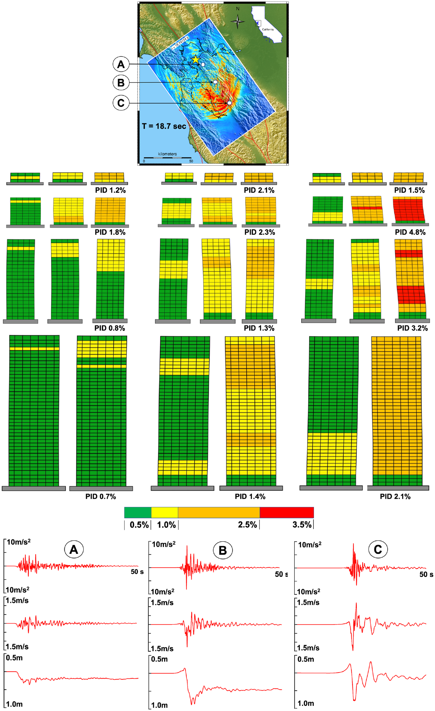
Intra-event site-to-site variability of building response: snapshots of building story drift limit states at all three sites (steel frame drift limit states from ASCE 43-19).
For all four buildings, the observed damage progressively increases as the building site moves toward the southern end of the fault, particularly for the 9, 20, and 40 story buildings. From the animations of the ground motions and the time history plots of the ground motions, in Figure 18, it is clear that a strong rupture directivity is taking place and a large fault-normal ground motion pulse is building toward the southern end of the fault. As a result, PID for a building sited to the south can easily be a factor of 4 or 5 greater than a building site closer to the hypocenter in the north which is significant considering this illustrates the demands for an identical building, located an identical distance off the fault and subjected to the same identical event.
This highlights the strong site variability of ground motion in the near-field driven by source effects, and the need to fully understand the implications of this intra-event variability when striving for optimal earthquake resilient design. The end-to-end simulation example illustrated here fully utilized the ecosystem and workflow illustrated in Figures 2 and 4. The ground motion simulations were completed on the Frontier system at OLCF, for a 10-Hz simulation, the 9.42 billion ground surface time histories consisting of 267 TB of data that were compressed into a 6.68 TB HDF5 file. The HDF5 data was chunked into 2 GB files for parallel transfer across the ESNET optical network requiring just 8 min and 38 s from ORNL to LBNL, including a check on the accuracy of transferred data integrity. With the ground motion data stored at LBNL, selected building simulations can be performed on demand on the Perlmutter GPU-accelerated system.
As a second example illustrating inter-event variability, two representative M7 Hayward fault rupture realization simulations are shown in Figure 19. The first realization consists of a rupture with a northern hypocenter and the second realization consists of a rupture with a southern hypocenter and a strong rupture directivity effect is evident in the wave stacking for each of these events. To provide insight into the inter-event variability of building response between these two realizations, the representative 3, 9, 20, and 40 story steel moment frame buildings were analyzed at all surface sites separated by 2 km spacing throughout the domain. For the fault-normal component of motion, the site-specific PID limit state contours for all four buildings are shown for the northern and southern hypocenter events in Figure 20. The very strong influence of rupture forward directivity leading to more damage to the south for a northern hypocenter and more damage to the north for a southern hypocenter is evident. Also shown in Figure 20 is the ratio of the maximum PID to the minimum PID for the two events at each site in the domain. The plots illustrate that for the two identical magnitude earthquakes, there are major building demand differences near the ends of the fault.
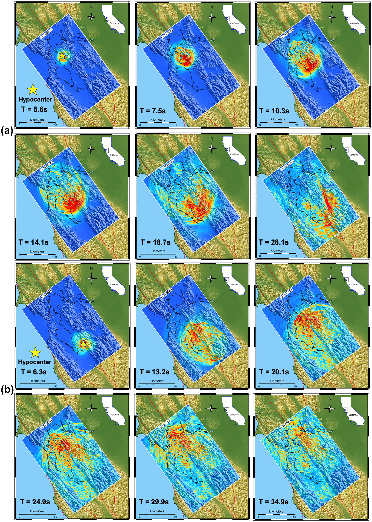
Time snapshots of seismic wave propagation for a Hayward fault rupture: (a) northern hypocenter; (b) southern hypocenter.
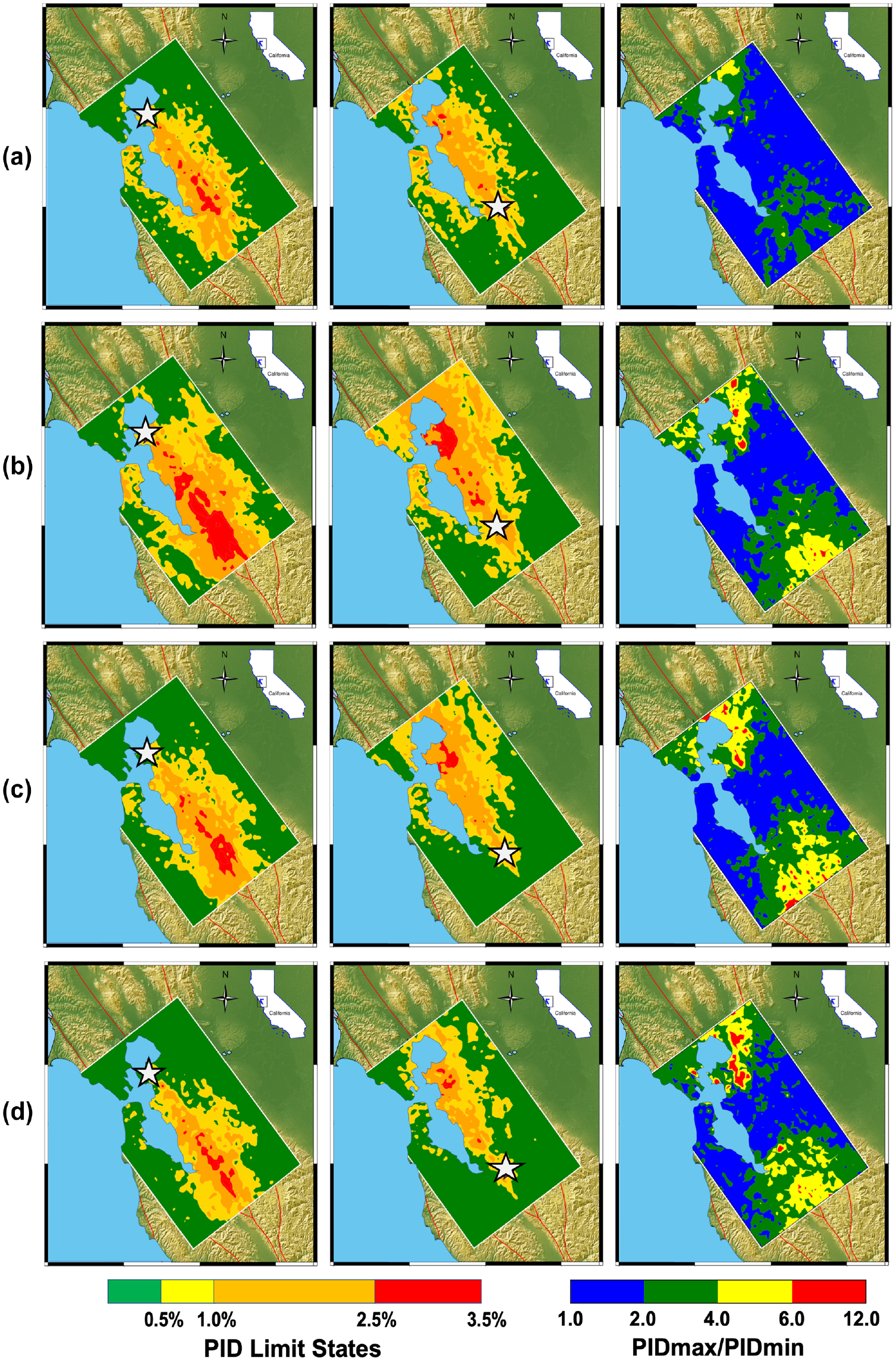
Inter-event PID building response to fault-normal motion for two Hayward fault rupture realizations: (a) 3 story steel moment frame; (b) 9 story steel moment frame; (c) 20 story steel moment frame; (d) 40 story steel moment frame, white star shows hypocenter.
For the northern hypocenter, the region of higher damage is heavily biased toward the south and the south bay cities including San Jose, while for the southern hypocenter, the damage is heavily biased toward the north and the cities of Berkeley and Oakland. The ratio of building maximum PID to minimum PID between these two realizations can be up to a factor of 12 near the ends of the fault, which adds emphasis to the need to consider a full suite of rupture realizations in evaluating the potential damage for a given scenario earthquake event.
Large, rare event simulations with the exascale ecosystem
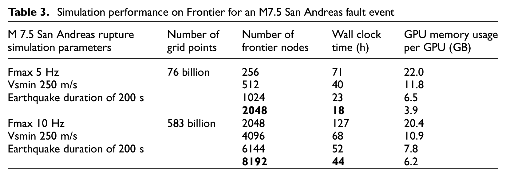
With the EQSIM completion of all DOE performance objective requirements, there was an opportunity to explore the limits of regional simulations for rare larger events on Frontier. For this example, the computational domain was expanded to encompass an M7.5 San Andreas fault earthquake as shown comparatively to the Hayward fault domain in Figure 21. The San Andreas model is substantially larger than the Hayward fault model and the duration of this M7.5 event is 200 s compared to the Hayward M7.0 duration of 90 s. For this simulation, a Graves and Pitarka San Andreas rupture model was generated for 200 km of the San Andreas fault including some local high-slip patches as shown in Figure 21. Time snapshots of the San Andreas event and ground motions at four selected sites, which exhibit the strong site-dependent characteristics of the ground motion waveforms, are shown in Figure 22. Site 1 and site 2 are situated in local basins in Santa Rosa Valley and the Livermore Valley, respectively. The simulated ground motions at both sites exhibit low accelerations and long duration motions that include long period, relatively large amplitude ground displacements associated with basin trapped waves. These motions starkly contrast with the near-fault motions at sites 3 and 4, each situated 2 km off the fault, where short duration strong fling-step and fault-normal pulse motions are evident.
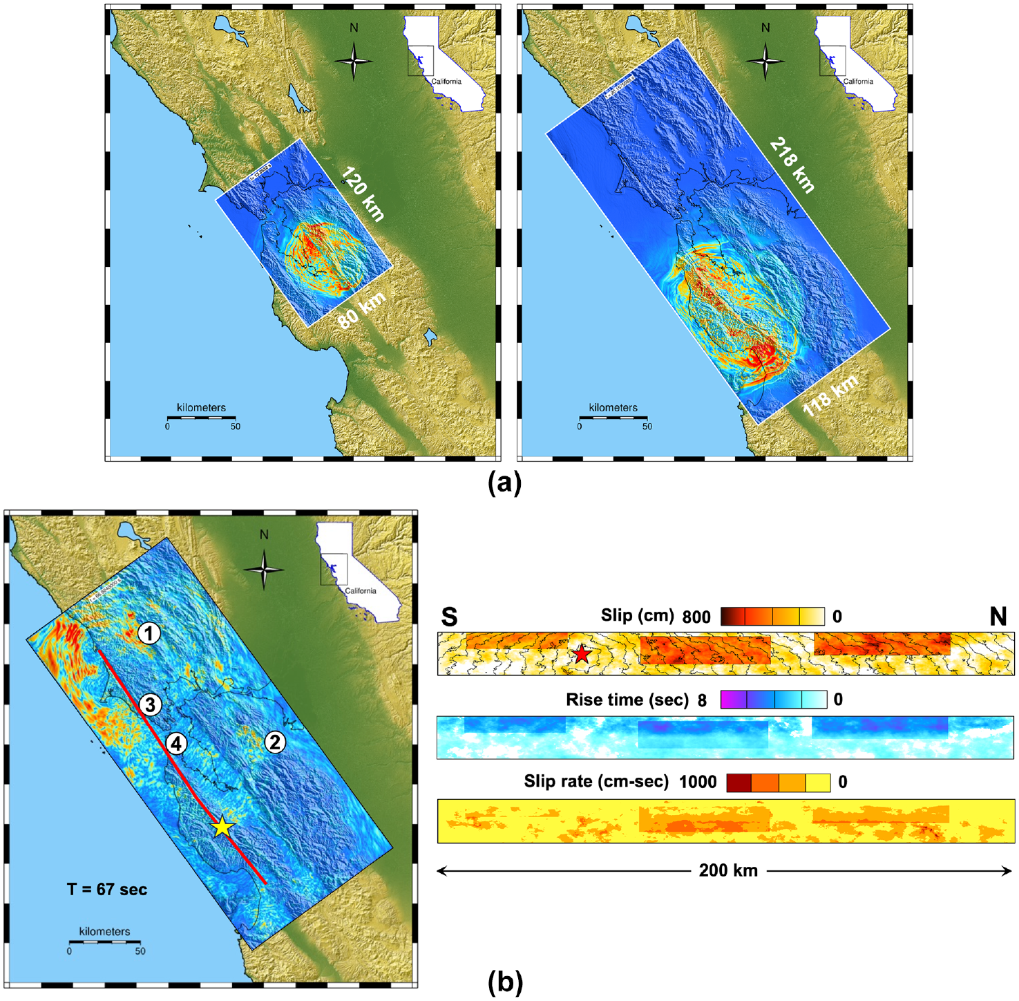
Computational domain for M7.5 San Andreas fault simulations and ground motion sites: (a) comparative domains for M7 Hayward fault and M7.5 San Andreas fault simulations; (b) Graves–Pitarka kinematic rupture model with large slip patches.
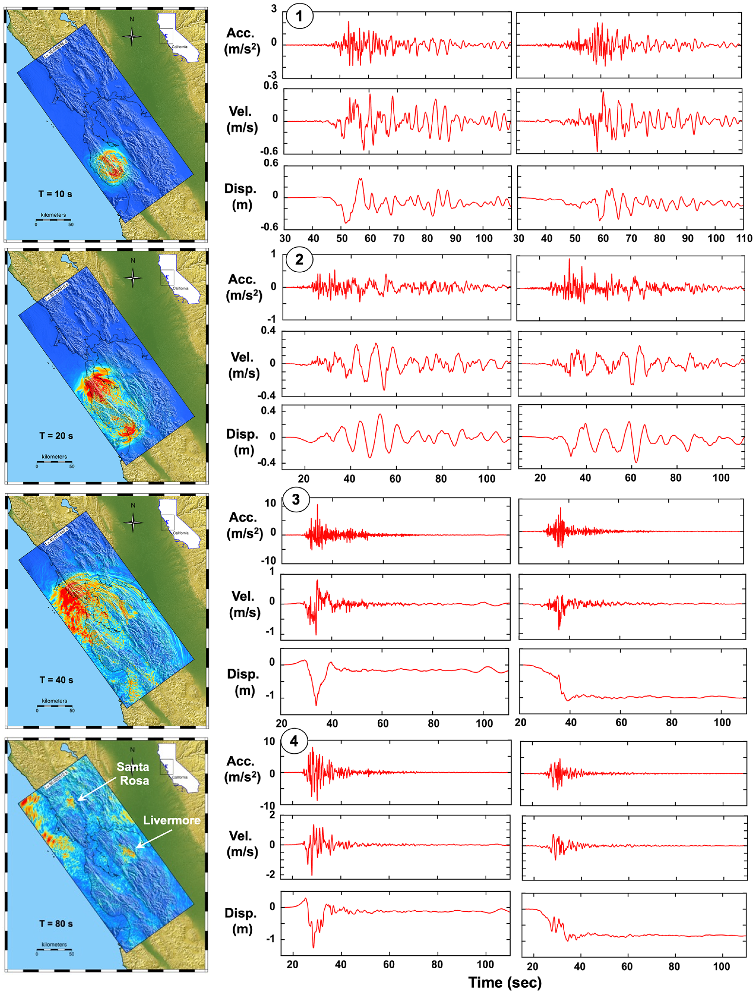
M7.5 San Andreas fault rupture simulation and ground motion waveforms at selected sites including both near-fault and distant basin sites.
The fault-normal ground motion pulses in the near-field of this simulated event exhibit an exceptionally sharp displacement pulse in the fault-normal direction. Recent near-fault ground motion data from the 2023 M7.8 Turkish earthquake for sites in the forward-directivity direction demonstrate very similar waveforms with a very sharp fault-normal pulse. The Frontier compute times for this large domain are summarized in Table 3 where the wall clock time for a 5-Hz resolution simulation is 18 h using 2048 nodes and the wall clack time for a 10-Hz simulation is 44 h using 8192 nodes.
Simulation performance on Frontier for an M7.5 San Andreas fault event
Discussion and summary
The transition to GPU-accelerated systems and the development of carefully designed and platform-validated high-performance workflow for the DOE exascale ecosystem has created a major leap forward in regional-scale, fault-to-structure earthquake simulations. The ability to compute earthquake simulations at frequencies of relevance to engineered systems, to resolve the velocity structure of soft near-surface sediments and to compute multiple event realizations within manageable compute times can be achieved on the latest exascale platforms. To provide additional context to the computational performance improvements, Figure 23 summarizes the full history of all earthquake simulations that have been performed by various research groups in the SFBA starting with the first simulation performed in 1999. This plot is based on the fact that for a uniform size grid, the computational effort dependency for a regional simulation can be shown to be proportional to the following parameters:

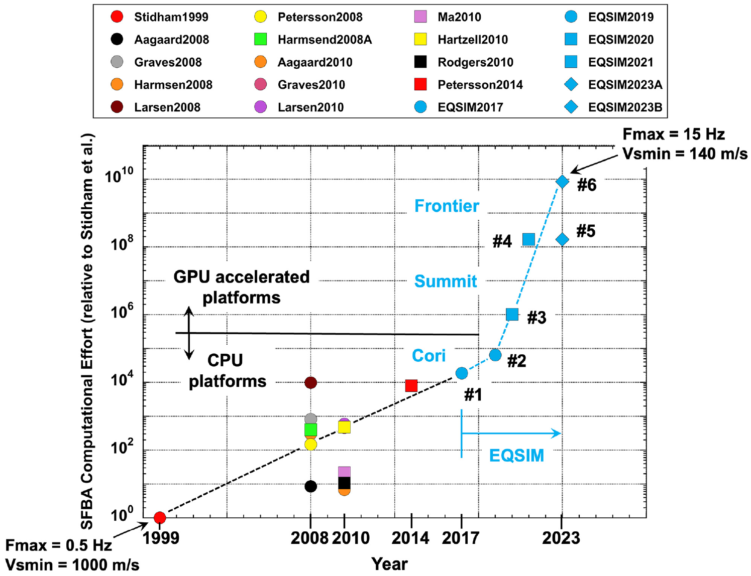
Computational effort associated with the entire history of SFBA simulations.
In Figure 23, the computational effort of each simulation is computed relative to the first SFBA simulation performed by Stidham et al. (1999). The increase in slope in Figure 23, after the transition from CPU (Cori) to GPU-accelerated systems (Summit and Frontier), illuminates the increased performance realizations of this new class of systems. These recent simulation advancements have removed much of the barriers to performing regional simulations at frequencies relevant to engineered infrastructure and the workflow described herein provides a user framework to execute these simulations efficiently on a routine basis. It is noted that there are important computational challenges with even larger domains (e.g. an M9 Cascadia event) so additional scaling needs to be explored. In upcoming studies, the EQSIM framework is going to be applied to large events in the New Madrid region of the Midwestern US and given the low seismic attenuation of Midwest shallow crust, this will necessitate exploration of even larger computational domains. To fully realize the benefits of a simulation-based virtual earthquake environment in support of new understanding and earthquake hazard and risk assessments, the computational performance achieved places a premium for continued improvements of regional geologic models and location-specific fault rupture scenarios to fully inform and constrain this new ecosystem for earthquake simulations.
In terms of workflow, development remains to be done to establish the most effective computational schemes for full incorporation of general nonlinear behavior in the near-surface geotechnical layer, and while the DRM approach implemented in EQSIM is one option, there are a number of alternatives that need to be thoroughly explored for computational efficiency.
Footnotes
Acknowledgements
The work was performed at the Lawrence Berkeley National Laboratory and Lawrence Livermore National Laboratory under DOE Contract DE-AC52-07NA27344. Exceptional support from the National Energy Research Scientific Computing Center at LBNL and the Oak Ridge Leadership Computing Facility at ORNL are gratefully acknowledged. Computational access and bank time for the Frontier system was provided by the DOE Innovative and Novel Computational Impact on Theory and Experiment (INCITE) program, which was essential to the completion of this work and gratefully acknowledged.
Declaration of conflicting interests
The author(s) declared no potential conflicts of interest with respect to the research, authorship, and/or publication of this article.
Funding
The author(s) disclosed receipt of the following financial support for the research, authorship, and/or publication of this article: This research was supported by the Exascale Computing Project (ECP; Project No. 17-SC-20-SC), a collaborative effort of two US Department of Energy (DOE) organizations - the Office of Science and the National Nuclear Security Administration.