
Abstract
The 30 November 2018, magnitude (Mw) 7.1 earthquake in Southcentral Alaska triggered substantial landslides, liquefaction, and ground cracking throughout the region, resulting in widespread geotechnical damage to buildings and infrastructure. Despite a challenging reconnaissance and remote-sensing environment, we constructed a detailed digital inventory of ground failure associated with the event from several sources. Sources included information derived from remotely sensed data, and data compiled from literature, social media postings, and earthquake damage information compiled by local, state, and federal agencies. Each instance of ground failure within the inventory contains information on the location and type of observed ground failure, and the methods and data used to document the occurrence. Where high-quality data, such as LIDAR or satellite imagery, were available and showed the ground-failure instance clearly, the extent is mapped as a polygon or polyline. All other locations are mapped as points. There are a total of 886 ground-failure instances documented within the inventory (400 landslides, 286 liquefaction features, and 200 features unattributed to specific processes). A semi-quantitative confidence scheme is used to describe mapping certainty associated with each ground-failure feature. This inventory represents a relatively moderate ground-failure-triggering event that occurred in a subarctic environment. This data paper describes the content within the inventory, the inventory data collection procedures, and limitations of the data. Events of this type are not often documented in detail; thus, adding the inventory data to the US Geological Survey Open Repository of Earthquake-Triggered Ground-Failure Inventories further diversifies the datasets available to the scientific community to be used to better understand and model earthquake-triggered ground failure.
Keywords
Introduction
Our understanding of earthquake-triggered ground failure, and our ability to model, mitigate, and respond to the associated hazard, is shaped by the quality of ground-failure observations collected after an earthquake (e.g. Brandenberg et al., 2020a, 2020b; Holzer, 1992; Keefer, 1984; Nowicki Jessee et al., 2018; Rodríguez et al., 1999; Tanyaş et al., 2017; Tuttle and Barstow, 1996; Zhu et al., 2017). Such observations are typically documented in inventories, which are databases containing detailed information on the occurrence, location, and attributes of ground failure associated with a particular earthquake (e.g. Harp et al., 2011). The US Geological Survey (USGS) currently maintains a repository of earthquake-triggered ground-failure inventories that spans decades and is updated with new inventories as they become available (Schmitt et al., 2017). Inventories in the repository are produced by the USGS and by other researchers who are willing to contribute their inventories to the effort.
The inventories in the repository were used in the development of the empirical landslide and liquefaction models that form the basis of the USGS ground-failure (GF) product, which is the first near-real-time product that estimates the spatial occurrence of landslide and liquefaction hazard after an earthquake (Allstadt et al., 2021; Nowicki Jessee et al., 2018; Zhu et al., 2017). The product provides situational awareness to the general public, media, emergency responders, and local agencies immediately after an earthquake (Allstadt et al., 2021). The repository is also being used to develop the next generation of geospatial ground-failure models (e.g. Aguilera et al., 2022; Geyin et al., 2022; Hamburger et al., 2021; Nowicki Jessee et al., 2020). Expanding the global repository of earthquake-triggered ground-failure inventories will not only improve our understanding of earthquake-triggered ground failure but it will also subsequently increase the quality of rapid-response tools, such as the USGS GF product.
The 30 November 2018, magnitude (Mw) 7.1 earthquake in Southcentral Alaska was one of the first domestic events to occur since the Fall 2018 deployment of the USGS GF product (Thompson et al., 2019). The earthquake slip distribution extended from about 45 to 65 km depth along a north–south striking normal fault that ruptured within the underthrust Pacific plate (Liu et al., 2019; Thompson et al., 2019; U.S. Geological Survey (USGS), 2018). Available data made it difficult to determine which of the moment tensor nodal planes ruptured. The original USGS solution preferred the eastward-dipping fault plane, while Liu et al. (2019) preferred the west-dipping plane. Initial observations of ground failure (Grant et al., 2020a; Jibson et al., 2019) showed that qualitatively, the product accurately highlighted many areas of landslide and liquefaction occurrence, although there were many instances where the model overpredicted or underpredicted the occurrence of ground failure (Thompson et al., 2019). However, there is uncertainty in this initial assessment of the product’s performance because only imprecise geotags of field observations and photographs were available at the time, not an actual ground-failure inventory that would have allowed for quantitative comparison (Thompson et al., 2019). Although developing a complete ground-failure inventory is already an arduous task, doing so for this event was particularly challenging because fresh snowfall and lack of sunlight at that time of the year limited initial field reconnaissance efforts (Grant et al., 2020a, 2020b) and hampered the visibility of ground-failure features in satellite imagery. In addition, many of the liquefaction features were ephemeral and only observed because of the rapid reconnaissance efforts. For example, sand boils that occurred on tidal flats were eventually washed away after subsequent tidal cycles. Despite these challenges, we developed a detailed ground-failure inventory associated with the event by drawing on a variety of mapping methods and data sources. To do so, we first performed a formal assessment to determine which remote-mapping methods would be more successful for this event and used that knowledge to guide our mapping efforts. Details on this assessment can be found in the work by Martinez et al. (2021). In this data paper, we describe the data and methods used to create the full inventory of earthquake-triggered ground failure associated with the 2018 Mw 7.1 earthquake in Southcentral Alaska, followed by a brief overview of the inventory and a discussion about the limitations of the dataset. The inventory data associated with this paper are available through a USGS data release (Martinez et al., 2022) and are integrated into the USGS Open Repository of Earthquake-Triggered Ground-Failure Inventories (Schmitt et al., 2017).
Data sources and methods
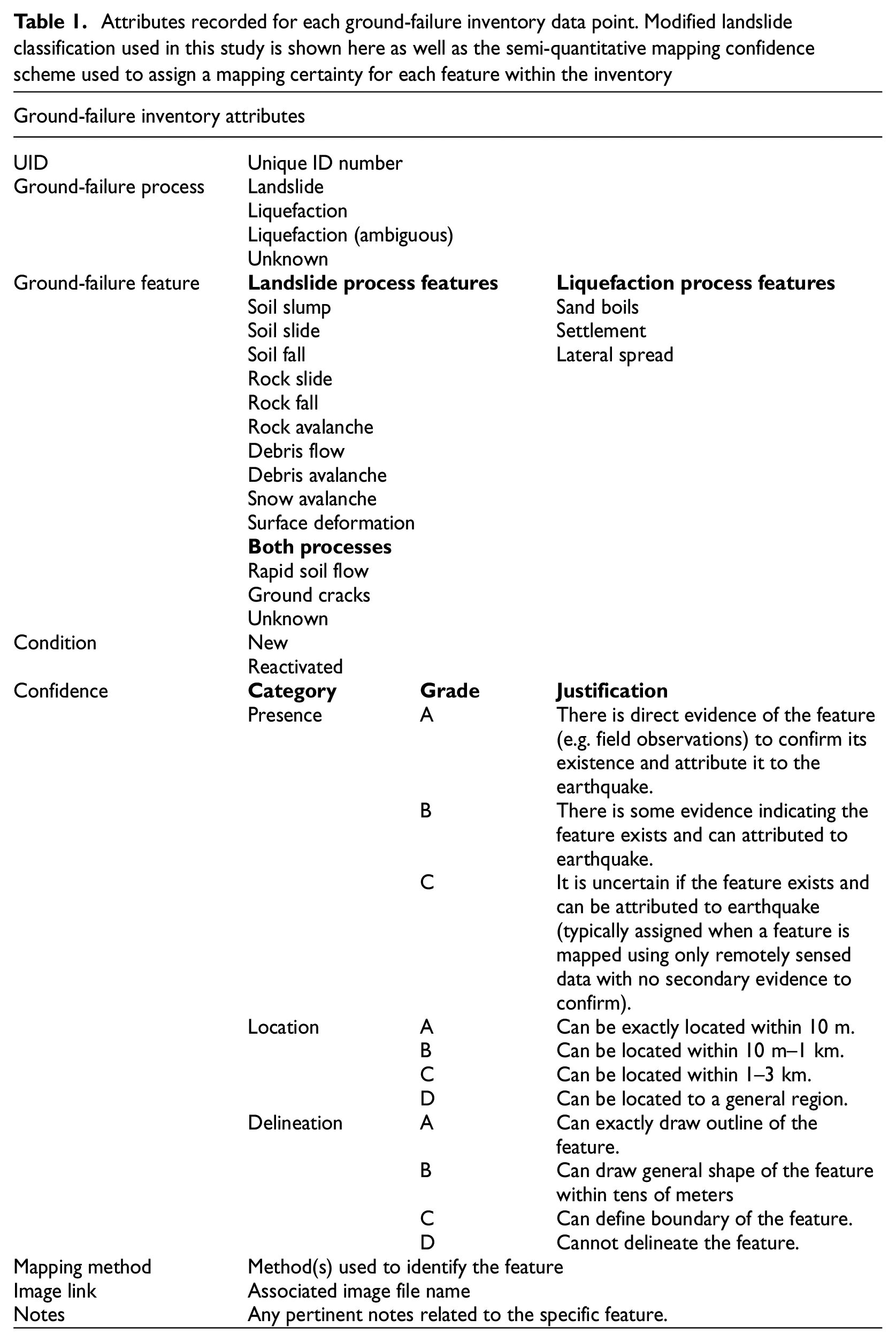
To develop our inventory, we carefully documented ground-failure occurrence as a point corresponding to the location of occurrence. Where possible, the spatial extent of the features was more precisely mapped with an additional polygon and or line feature. We placed the data points near the headscarp or initiation point of the observed landslide features. For liquefaction data, we placed the point in the center of the feature. We carefully recorded information related to each ground-failure occurrence in the attribute table associated with the point file of the inventory. Details on the recorded information associated with each data point can be seen in Table 1. Below, we describe the data and methods used to identify and map the occurrence of ground failure, followed by an explanation of our classification protocol and discussion on how we communicate uncertainty associated with each data point. The inventory data associated with this paper are available through a USGS data release (Martinez et al., 2022) and are integrated into the USGS Open Repository of Earthquake-Triggered Ground-Failure Inventories (Schmitt et al., 2017).
Attributes recorded for each ground-failure inventory data point. Modified landslide classification used in this study is shown here as well as the semi-quantitative mapping confidence scheme used to assign a mapping certainty for each feature within the inventory
LIDAR-derived digital elevation model differencing
High-resolution digital elevation models (DEMs) are typically used to develop ground-failure inventories due to their ability to display the ground surface with enough detail to delineate landslide (e.g. Harp et al., 2011) and, in some instances, liquefaction features. Differencing pre- and post-earthquake DEMs is particularly useful as it can identify previously unmapped or unobserved features and aid in volumetric analyses (e.g. Kallimogiannis et al., 2022). As such, we began our ground-failure mapping efforts by first differencing the high-resolution pre- and post-earthquake light detection and ranging (LIDAR)-derived DEMs available from the Alaska Department of Natural Resources (AK DNR) Division of Geological and Geophysical Surveys (DGGS) elevation portal (DGGS Staff, 2013). The pre-earthquake LIDAR used to develop the inventory was collected in 2015, and the post-earthquake LIDAR used was collected shortly after the earthquake in 2018. Both LIDAR-derived DEMs have a spatial resolution of 1 m. The align tool within the QGIS software (Version 3.10) was used to align the DEMs to one another for the purpose of differencing. The tool reprojects input raster files to the same coordinate reference system and resamples them as needed for alignment. The aligned DEMs were differenced to create a map displaying changes in elevation that occurred from 2015 to 2018 (refer to Martinez et al., 2021 for more details). The LIDAR-derived DEMs vary in their extent and have an areal overlap of approximately 321 km2, which covers only 0.5% of the area that experienced moderate to very strong shaking (Modified Mercalli intensity V–VII) during the earthquake (60,690 km2) as estimated from the USGS ShakeMap Atlas v4 (Figure 1) (Marano et al., 2024).
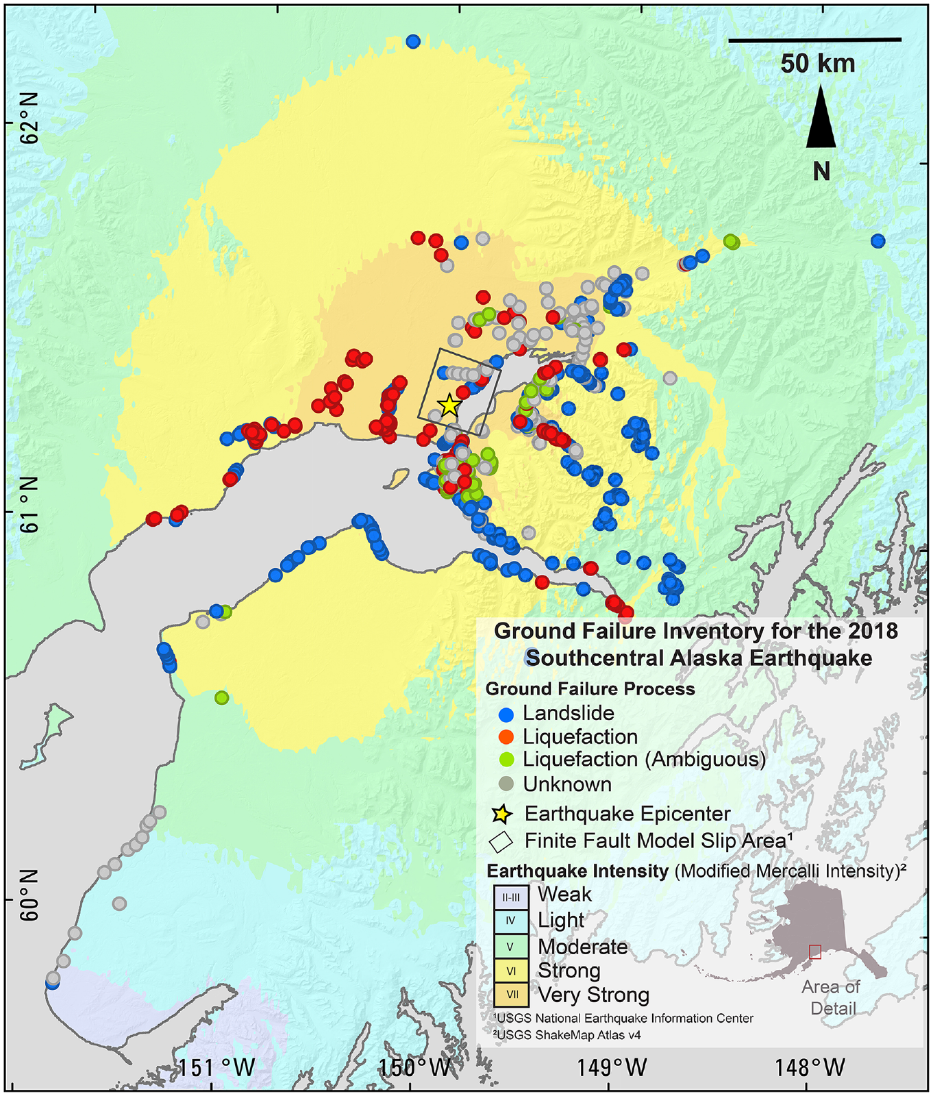
Ground-failure inventory for the 2018 Southcentral Alaska M7.1 earthquake. Inventory is overlain on the USGS ShakeMap (Atlas v4) shaking intensity model associated with the earthquake event. From Martinez et al. (2022).
Multispectral and optical imagery
In regions lacking sufficient DEM coverage, we used normalized difference vegetation index (NDVI) differencing to identify and map ground failure. NDVI maps are derived from multispectral imagery and display the relative health or existence of vegetation in a landscape (Rouse et al., 1973). For this study, we derived NDVI maps using imagery from the European Space Agency’s Sentinel-2 (S2) Multispectral Instrument (MSI) (Drusch et al., 2012). Ground failure that disturbs vegetation can be mapped by differencing pre- and post-earthquake NDVI maps. However, NDVI maps of the landscape immediately following the earthquake were of limited usefulness due to snowfall that occurred shortly after the earthquake (2 December 2018). To overcome this limitation, we used Google Earth Engine (Gorelick et al., 2017) to create composites of multispectral images of the summers (May 1 to July 30) before and after the earthquake. The seasonal composites were then used to create NDVI maps that were differenced to determine where there were any substantial changes in vegetation that could potentially correspond to ground failure. The downside to this approach is that those landslides or other vegetation changes found within that timeframe may not all have been caused by the earthquake. Where possible, instances of ground failure identified using the NDVI method were verified using other data sources (e.g. field observations). Although the resolution of the data used for the NDVI differencing (10 m) is lower than that used for DEM differencing (1 m), the NDVI data are advantageous to use because the imagery used to generate NDVI from Sentinel-2 data is available globally, and thus, for the entire earthquake-affected region of Southcentral Alaska.
When possible, optical satellite and aerial imagery were also used to map ground-failure features. However, in most instances, the imagery alone, even if of high-spatial resolution, could not capture the often-subtle features that were identified on the ground during field reconnaissance (e.g. minor ground cracks, smaller riverbank slope failures). In addition, visibility of the ground surface was limited in satellite imagery because of snow fall that occurred shortly after the earthquake. Some features, such as large road cracks, were not visible following snowmelt because they were quickly repaired. Other ephemeral features, such as sand boils or cracks on tidal flats, were no longer visible in satellite imagery after snowmelt and several tidal cycles.
Field observations and supplemental information
Remotely sensed data alone were found to be insufficient for mapping ground failure associated with this event (Martinez et al., 2021). Thus, in addition to the remotely sensed data, the inventory field observations gathered by the USGS contributed greatly to the inventory (Grant et al., 2020b). Using the global positioning system (GPS) coordinates of geotagged photographs and reference points visible in both satellite or aerial imagery and the photographs, the location of the observed ground failure was mapped as precisely as possible.
While field observations made by the USGS were useful to map ground failure that could not be observed via remotely sensed data alone, the coverage was mostly limited to areas that were accessible on the ground and that field teams had time to visit. Fresh snowfall also obscured ground failure in some areas during the field campaign. As such, we used additional information from a variety of other sources to develop the inventory. For example, information on earthquake damage compiled by the state of Alaska, local boroughs (Municipality of Anchorage, Kenai Peninsula Borough, Matanuska-Susitna Borough Department of Emergency Services), and Federal Emergency Management Agency (FEMA) Region 10 was shared with us. This information was originally compiled from reports of earthquake damage made by homeowners impacted by the earthquake; where these reports were detailed enough, we could use the information to document specific instances of ground failure. Similarly, the Alaska Department of Transportation and Public Facilities (AK DOT & PF) documented earthquake damage to road infrastructure across the state and organized this information within an internal database containing information on the location of the damage and associated photos. The AK DOT & PF allowed us to use their internal observations to populate our inventory as well. For both databases, locations were sometimes provided as addresses or coordinates, while others had to be manually determined via aerial imagery and photo comparison. Where location information was not possible to determine precisely, ground failure was still documented while noting that our confidence in the location was low. Through email correspondence with the 673 Civil Engineers Squadron at the Joint Base Elmendorf–Richardson and Anchorage Fire Station 12, we were also able to document ground failure that occurred at those facilities. Social media information related to earthquake damage compiled by Luke Blair and Alexandra Pickering (2018 Alaska Earthquake Virtual Clearinghouse website, n.d.), and data from literature on the 2018 earthquake event were also used to document ground failure. Table 2 provides detailed descriptions of each data source.
Detailed information on data sources used for the ground-failure inventory
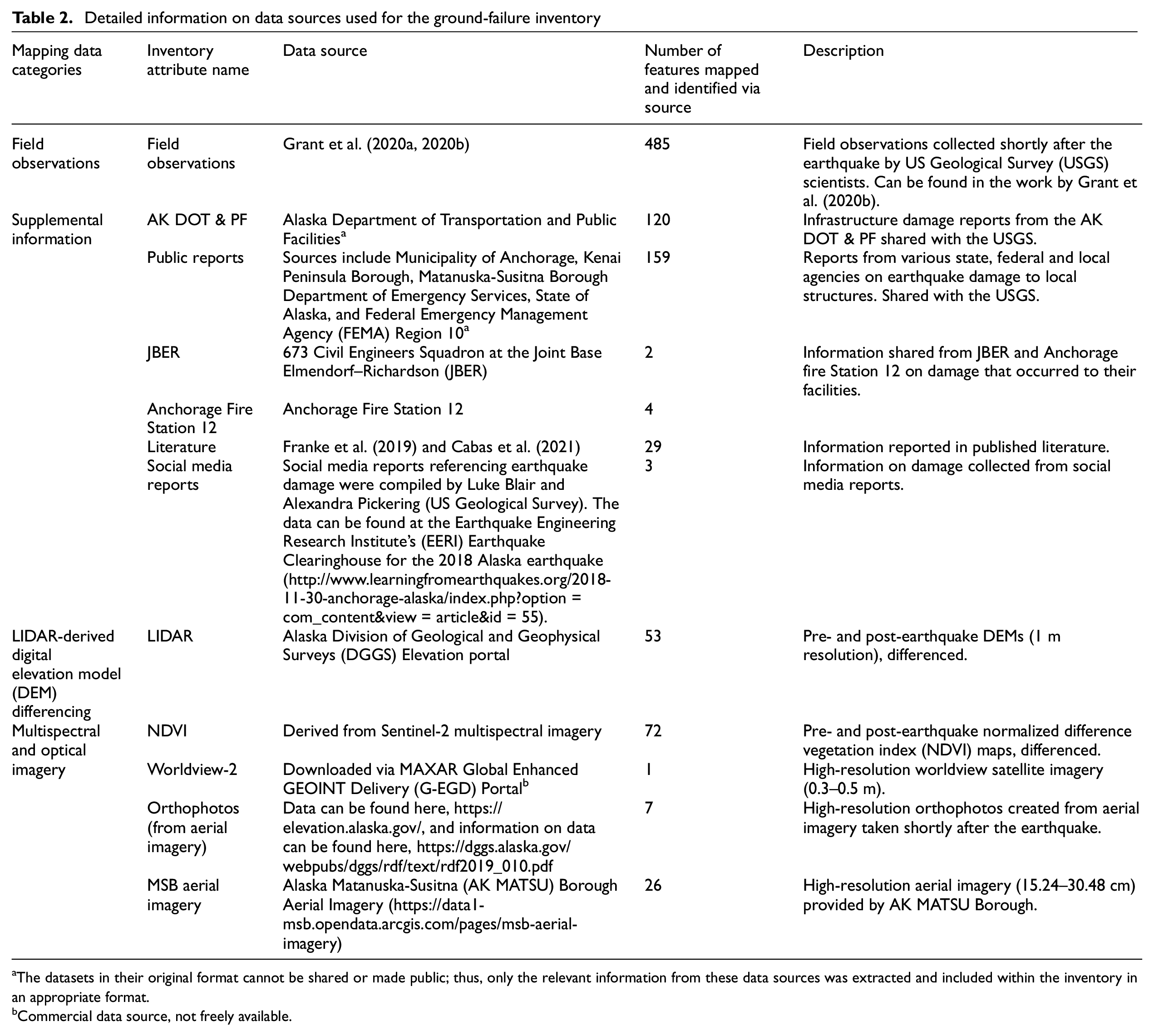
The datasets in their original format cannot be shared or made public; thus, only the relevant information from these data sources was extracted and included within the inventory in an appropriate format.
Commercial data source, not freely available.
Ground-failure classification
For each instance of ground failure, the description of the physical feature is recorded directly and, where possible, is categorized based on the process interpreted to have caused it (landslide, liquefaction). We inferred which ground-failure process to assign to each ground-failure location based on contextual information, such as the environment and presence of evidence, that indicates ground failure may have occurred. Our ability to adequately infer what ground-failure processes occurred depends largely on the quality and availability of data in the affected area and whether the site was visited in the field.
We assigned the “landslide” process to locations where there are indications of the downhill movement of material. This designation is often straightforward for more rapid, disrupted slides that showed signs of fresh movement. In the field, this consisted of features, such as newly exposed unweathered rock, fresh talus, and dust on snow, recently living vegetation damaged or buried under rocks or soil, distinct cracks, blocks, and fissure zones with sharp edges that stood out even with snow cover present. Remotely sensed landslides were classified as such based on the surrounding topography and shape of the landslide and confirmation of new movement by comparison against pre-event imagery. There are, however, downslope movements that are more subtle in the landscape that may be less straightforward to classify. For example, for incipient landslides, the only field indication of their existence may consist of fissures or ground cracks near the top of a slope and vegetation may preclude detection or characterization by remote-sensing methods. Field observations were more helpful in identifying evidence of small and shallow landslides. Remote-sensing techniques can be used to identify landslides in areas that are less accessible or less likely to be observed in the field by a human.
Adequately classifying the type of landslide is dependent on the ability of the mapper to determine the material involved and the style of movement of that material. Those characteristics (material, movement) can be challenging to identify, especially for features not visited in the field. Here, we use a modified classification scheme based on the work by Keefer (1984) to classify the landslides within our inventory (refer to Table 1 for an overview of the modified classification scheme). Our ability to classify landslides was highly dependent on the data sources used to map the landslides. An example of a feature that could be adequately classified is feature 26, which is shown in Figure 2b. We can infer that the soil moved downslope in a translational manner because the field photos (Figure 2d) show that only the uppermost layer of the soil was affected, and the differenced DEM data (Figure 2b) show both some erosion of material and deposition down slope. In other cases, data available were not sufficient to identify the material involved or the movement of that material. In these cases, we inferred the landslide type based on external evidence, such as the proximity of the feature to others that were confidently classified. This was typically the case for landslides along the coastal bluffs or riverbanks, as it can be reasonably assumed that similar processes are occurring in the same environment. Where additional information or context was lacking, the landslide feature was labeled as “unknown.” In some cases, it was difficult to discern landslide from liquefaction processes. For example, the language used by homeowners to describe damage to their property was sometimes ambiguous. In this case, we infer that the damage incurred on slopes corresponded to ground failure as a result of landslide processes and those in low-lying areas occurred as a result of liquefaction processes.
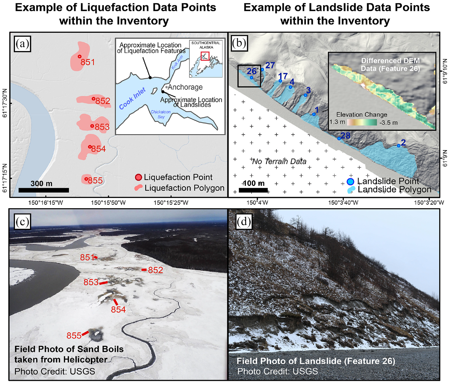
Examples of liquefaction and landslide inventory data: (a) liquefaction points and polygons are shown for sand boils that were mapped on the Cook Inlet tidal flats, (b) landslide points and polygons are shown for landslides mapped along the coastal bluffs of southern Anchorage. The differenced DEM data for feature 26 are also shown in an inset map for comparison to the field photograph, (c) field photograph of the mapped sand boils. Each sand boil is labeled with the Unique ID that corresponds to the associated ground-failure inventory data point and (d) field photograph for one of the landslides mapped along the coastal bluffs of southern Anchorage (feature 26).
Evidence that liquefaction occurred includes the presence of ground cracks, sand boils, lateral spreads, the settlement of structures, and rapid soil flows. Cyclic softening of fine-grained soils possibly produced some of these features (Boulanger and Idriss, 2006). Without site-specific knowledge of each feature, it is not possible to differentiate between liquefaction and cyclic softening failures in many cases. We infer the occurrence of liquefaction based on the evidence available and our knowledge of the study area. In cases where direct evidence of liquefaction is lacking (i.e. sand boils), the classification is based on the proximity to identified sand boils (within 100 m). Liquefaction was interpreted to be the process for lateral spreading features parallel to water bodies. Low-lying features on flat slopes for which no additional evidence is available to indicate that liquefaction occurred are given the label “Liquefaction (Ambiguous)” to reflect the uncertain nature in their process designation.
Data quality
Each method used to map ground failure has specific limitations and strengths in terms of adequately documenting ground failure. For example, mapping a feature using DEM differencing typically results in high confidence in terms of the location and extent of the ground-failure feature. However, because the differencing procedure can highlight other changes in the terrain that are unrelated to earthquake-triggered ground failure, confidence in the presence of the ground-failure feature can be low when there is a lack of more direct evidence (e.g. field observations) to corroborate the existence of the ground-failure feature. Therefore, it is necessary to communicate mapping confidence for each data point in an objective manner, so that any person(s) attempting to use the inventory for data-driven analyses can filter the data based on their needs. For example, those attempting to determine what environmental parameters correlate to ground failure might like to only consider the points in which we are highly confident in the location. Similarly, someone attempting to understand what parameters might correlate with earthquake-triggered landslides may choose to filter out the dataset based on those with high delineation certainties.
To communicate confidence for each data point, we describe mapping certainty for each feature within the inventory by assigning a semi-quantitative grade (A through C or D) for three categories related to the certainty of (1) feature existence, (2) positional accuracy, and (3) mapped delineation quality. Those categories are denoted as “presence,”“location,” and “delineation certainty” within the inventory. For example, the landslide shown in Figure 2b and d (feature 26) was assigned a certainty grade of A for the presence, location, and delineation categories. The landslide shown in Figure 2 was assigned a high grade for all categories because there is direct evidence of its existence (i.e. it was observed and documented in the field), and the extent could be mapped in detail using the high-resolution differenced LIDAR-derived DEM. Similarly, the sand boils shown in Figure 2a and b were assigned an A grade for both the presence and location certainty categories because there is direct field evidence of sand boils (i.e. field photographs). They were assigned a delineation certainty grade of C, however, because their spatial extent was estimated and mapped visually using the field photograph as a reference. Grade definitions within each category are described in further detail in Table 1.
To minimize human error, two co-authors who did not contribute to the initial mapping carefully reviewed the inventory for inconsistencies and errors. The reviewers focused on capturing typos, missing data, mapping position errors, and inconsistently formatted information. They also flagged any landslides with questionable classifications for further consideration.
Summary of the ground-failure inventory
The final ground-failure inventory is composed of 886 points that each correspond to the location of earthquake-triggered ground failure associated with the 2018 event (Figure 1). Figure 3 provides an overview of the entire inventory. Figure 3a shows the number of ground-failure instances corresponding to a particular process, and Figure 3b shows the type and number of observed features within the landslide and liquefaction process categories. In some instances, we used many methods to identify and map a singular ground-failure feature. Field observations, for example, could help identify the location of a feature and the differenced DEM could be used to map the extent of the ground-failure feature more accurately. Figure 3d shows the number of ground-failure instances that we identified using each data source or method.
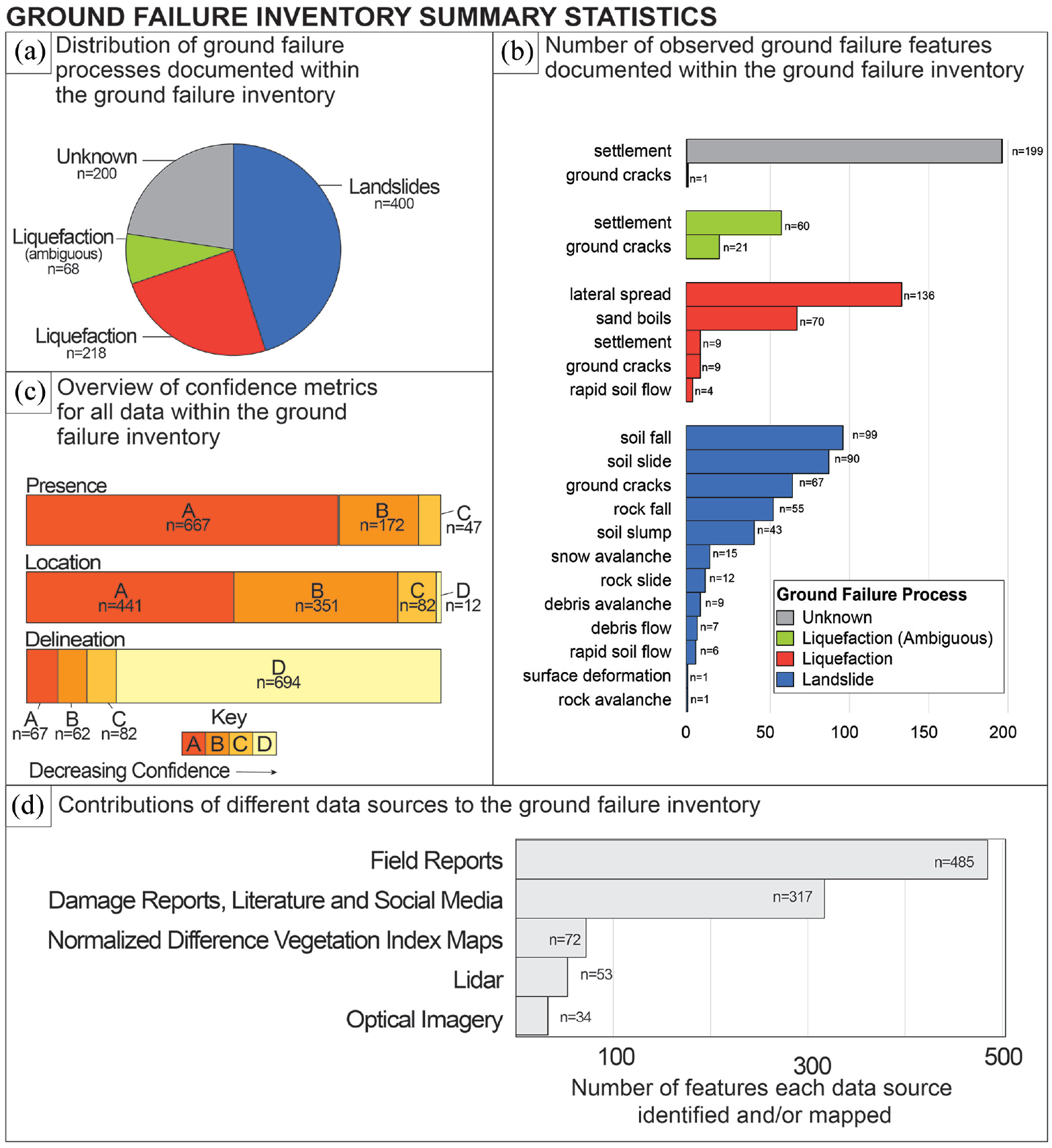
Summary statistics for the ground-failure inventory: (a) distribution of ground-failure processes documented within the inventory, (b) type and number of observed features within the landslide and liquefaction process categories. Colors indicate the categories shown in part (a), (c) summary of confidence metrics for all inventory data and (d) contribution from data sources used to identify ground-failure features. Shown here is the number of times each source contributed to identifying or mapping a feature. Some ground-failure features were identified or mapped using multiple data sources. For example, both field observations and LIDAR data could be used to fine-tune the location and extent of a mapped landslide.
Photographs of ground failure are included in the data release associated with this article (Martinez et al., 2022) and can be linked to map ground-failure instances within the inventory. Where applicable, the image file name is noted in a field that corresponds to the appropriate feature. The inventory and associated photographs are viewable via an ArcGIS interactive web map (https://doi.org/10.5066/P9457YU7). Note that not all ground-failure features within the inventory associated with this article were documented using photographs.
The inventory dataset can be downloaded from Martinez et al. (2022) as a zipped folder that contains the inventory shapefiles, associated photograph files, and XML metadata file. The shapefiles and photographs are contained in their own zipped folders. The shapefile folder contains a point, polyline, and polygon shapefile. The primary shapefile is the point shapefile as it corresponds to the mapped location of all ground-failure points within the inventory. Information associated with each point is documented in the attribute table of the point shapefile. Table 1 gives an overview of the information associated with each data point within the inventory. Additional polyline and polygon shapefiles exist for those features that could be more precisely mapped. Each individual ground-failure feature has a unique ID that is used to link the feature across all shapefiles (e.g. point, polyline, and polygon shapefiles). Detailed information on the dataset structure can be found within the metadata file, which can be accessed from Martinez et al. (2022).
Toward a more representative global repository of ground-failure occurrence
The USGS near-real-time GF product relies primarily on the models developed by Nowicki Jessee et al. (2018) and Zhu et al. (2017) to determine the probability of occurrence and spatial distribution of landslides and liquefaction, respectively. These models were both developed, tested, and validated using the data within the global repository of earthquake-triggered ground-failure inventories (Schmitt et al., 2017) and globally available proxies for susceptibility (e.g. lithology, compound topographic index, distance to water bodies, slope). The USGS GF product has proven useful in the qualitative assessment of ground-failure hazard and population exposure after earthquake events (Allstadt et al., 2021). This highlights the utility of the inventory data that underpins the ground-failure models. However, Allstadt et al. (2021) also noted that the model outputs generally overestimate the spatial extent of liquefaction and underestimate the areas impacted by certain landslide types. Some of these performance issues might reflect the bias in existing inventories toward exceptional ground-failure events (Allstadt et al., 2022; Tanyaş et al., 2017) or other biases in global representation. For example, Nowicki Jessee et al. (2018) found no statistical relationship between landslide location and several climatic factors (e.g. aridity, mean monthly precipitation) within the compilation of global inventories available at the time, despite hillslope water availability being a well-established major factor in slope stability. To improve earthquake-triggered ground-failure models, more complete inventories that represent the wide range of settings in which ground failure can occur globally would be useful.
The inventory presented here for the 2018 Anchorage earthquake represents a type of earthquake (deep, with relatively moderate ground motions) and setting (subarctic) not currently well represented in the global database. The earthquake also occurred when temperatures were near or below freezing. The inventory presented here can also help develop more accurate regional estimates of earthquake-triggered ground failure as there is currently only one ground-failure inventory in the repository associated with an earthquake in Alaska, the Mw 7.9 Denali earthquake in 2002, a much larger, shallower crustal primarily strike-slip earthquake that triggered a very different style of ground failure far from Anchorage (Gorum et al., 2014; Jibson et al., 2006). Our understanding of earthquake-triggered ground failure in Alaska, and especially around Anchorage, is largely based on what was observed after the devastating 1964 Great Alaska earthquake (Hansen et al., 1966). The ground failure triggered by that earthquake was vast, diverse in style, and widespread and was well documented but occurred in the pre-digital era, so no inventory exists. Therefore, this inventory can provide some insight on how ground failure is expressed in the same region, albeit after a smaller magnitude earthquake.
Limitations
Adverse environmental conditions including snow fall, limited daylight hours, a large earthquake-affected area, and accessibility constraints limited the extent to which both field and remotely sensed observations could be reliably used to compile a complete ground-failure inventory. To communicate this variability in the level of completeness and quality, Figure 4 displays the region, highlighted in white, in which direct observations of ground failure were made and where high-resolution pre- and post-earthquake LIDAR data are available. This higher-confidence mapping region displays where the inventory is considered complete and has high quality due to the nature of the data (i.e. direct observations, high-quality LIDAR) used for mapping in this region. Of note is that the lack of documented ground failure within Chickaloon Bay is likely not due to a lack of direct evidence, but rather the non-occurrence of ground failure in the bay. Ground failure was not observed in this area during field reconnaissance (Grant et al., 2020a), although one caveat is that tidal erosion may have removed any evidence of ground failure here if it existed. Although the inventory is considered incomplete, we provide sufficient information on certainty for each point and maps of areas that are complete so that potential users can select and use the data points that best meet their specific needs.
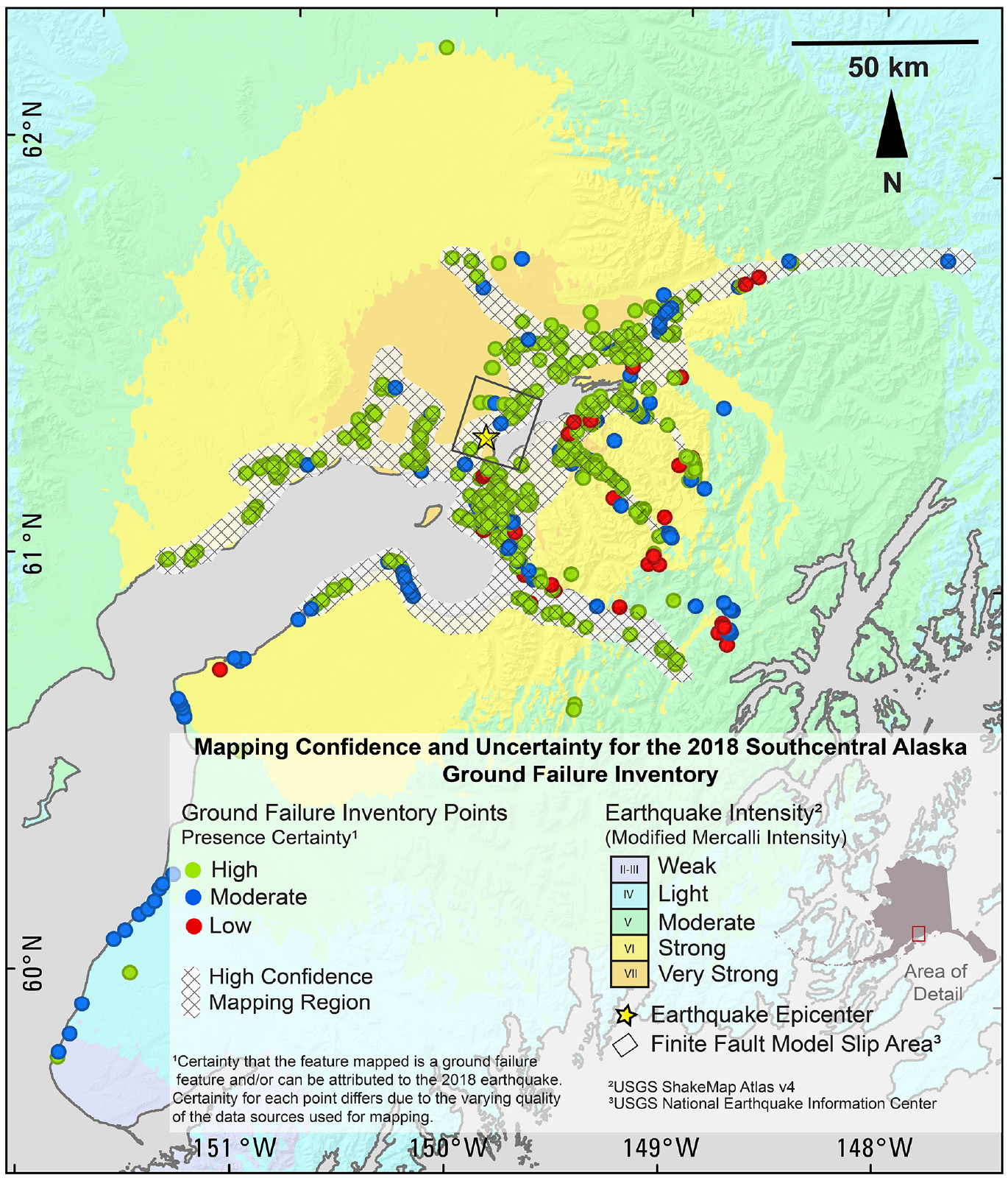
Hatched regions in white show areas of high confidence in inventory data. Refer to Grant et al. (2020a) for the location of ground and flight tracks. Direct ground and aerial observations, along with high-resolution (1 m) pre- and post-earthquake LIDAR for a portion of the area, all contribute to the higher confidence within this region. Individual points within the inventory have been assigned semi-quantitative certainty values (Table 1). Shown here is the presence of certainty which corresponds to the certainty the mapper has that the feature exists and that it can be confidently attributed to the earthquake.
Summary
Ground-failure inventories are one of the foundational datasets that underpin earthquake-triggered ground-failure models. We developed a detailed earthquake-triggered ground-failure inventory documenting, as completely as possible and using a wide variety of data sources, the ground failure triggered by the 2018 Southcentral, Alaska earthquake. This inventory adds to the continuously expanding global earthquake-triggered ground-failure repository while also highlighting the challenges faced with creating complete inventories. Specifically, this inventory illustrates the need to adequately describe confidence, both spatially (Figure 4) and for individual data points, so that future modeling efforts may benefit from understanding how inventory errors may propagate. Updating the global repository with data from a diverse set of events and including detailed completeness information, ultimately contributes to our understanding of and ability to respond to earthquake-triggered ground-failure hazards. It can also improve our understanding of earthquake-triggered ground failure within Alaska and our ability to adequately model ground failure within the region. To summarize, the data presented here can help improve global estimates of ground-failure occurrence and spatial distribution by diversifying the data within the global repository.
Footnotes
Acknowledgements
The authors thank Alex Grant, Rob Witter, and Randall W Jibson for their thoughtful contributions throughout the project and their contributions to the field observation database. In addition, they thank Kristen Keifer for her assistance with the Alaska Department of Transportation and Public Facilities (AK DOT & PF) database. Any use of trade, firm, or product names is for descriptive purposes only and does not imply endorsement by the US Government.
Declaration of conflicting interests
The author(s) declared no potential conflicts of interest with respect to the research, authorship, and/or publication of this article.
Funding
The authors disclosed receipt of the following financial support for the research, authorship, and/or publication of this article: This work was funded by the US Geological Survey.
Data and resources
The geographic information system (GIS) files, inventory photographs, and detailed metadata associated with the ground-failure inventory are available from the work by Martinez et al. (2022). Elevation data and orthophotos used can be downloaded via the Alaska Division of Geological and Geophysical Surveys (DGGS) Elevation Portal (https://elevation.alaska.gov/). Matanuska-Susitna Borough Aerial Imagery can be accessed at ![]() .
.